文化差異與動能投資報酬---由中國文化談起

(1)

行政院國家科學委員會補助專題研究計畫

▉ 成果報告

□期中進度報告

文化差異與動能投資報酬:由中國文化談起

計畫類別：▉ 個別型計畫 □ 整合型計畫

計畫編號：NSC 95－2416－H－004－026－MY2

執行期間：95 年 08 月 01 日至 97 年 07 月 31 日

計畫主持人：李怡宗

共同主持人：

計畫參與人員：

成果報告類型(依經費核定清單規定繳交)：□精簡報告 ▉完整報告

本成果報告包括以下應繳交之附件：

▉赴國外出差或研習心得報告一份

□赴大陸地區出差或研習心得報告一份

□出席國際學術會議心得報告及發表之論文各一份

□國際合作研究計畫國外研究報告書一份

處理方式：除產學合作研究計畫、提升產業技術及人才培育研究計畫、

列管計畫及下列情形者外，得立即公開查詢

□涉及專利或其他智慧財產權，□一年▉二年後可公開查詢

執行單位：

(2)

Abstract

Recent research documents the existence of momentum effects in stock returns in most of the Western countries. Recently, Hvidkjaer（ 2006 ） provides the first/only evidence that momentum effects are partly from the slowly underreaction of small traders to past returns, using transaction data. In contrast, there is no evidence that large traders react to past returns. A unique dataset from the Taiwan stock exchange allows us to address the momentum behaviors, by examining the order flow data for types of investors directly. Contrary to Hvidkjaer (2006), our paper document momentum behaviors for both institutional and individual orders from foreign investors. Domestic investors (including institutions and individuals, big and small traders) do not tend to sluggish reaction to past returns, and they do have significant impact on moving prices in the same direction. Interestingly, foreign investors tend to react to past returns significantly, while domestic investors only show slightly reaction on past return. Besides, small domestic individuals tend to be more contrarian than big domestic individuals. Therefore, it is still a puzzle about the rationales that may explain momentums.

(3)

Contents

Abstract ---II

Introduction---1

Data and Hypothesis---3

Empirical Results---5

Discussion and Conclusion---9

Reference---12

Figures and Tables---14

計畫成果自評---34

(4)

1. Introduction

Even market efficiency has been dominated finance economics throughout several decades, the unexplained persistence of momentum returns is one of the most serious challenges to the asset-pricing literature(Fama and French (1996)). However, the source of the profits and the interpretation of the momentum effects are widely debated, and it has attracted a lot of scholars search for the rationales.

Most of the scholars search for the rationales by borrowing theories from psychology such as representativeness, conservatism, overconfidence, and self-attribution, to explain the momentum profits (Odean 1998; Daniel, Hirshleifer, and Subrahmanyam 1998, Jegadeesh and Titman 2001). However, there is little direct evidence showing momentum effect is driven by any of the aforementioned psychology. Jaggedness and Titman (2001) argue that the momentum effect is likely to be caused by the delayed over-reaction by investors. Recently, Hvidkjaer（2006） provides a direct test of the relationship between underreaction and momentum effect recently. His findings indicate that momentum effects are partly from the slowly underreaction of small traders to past returns, using transaction data. In contrast, there is no evidence that large traders react to past returns.

By using order flow data, this paper contributes the following aspects. Firstly, If momentum are partly driven by underreaction of small traders to past returns, then we should expect to see that momentum phenomenon is prevailing in a market dominated by individual investors. In Taiwan, individual trading contributes to 70% to 90% of the total trading volume during past ten years. Hence, the Taiwanese market provides a good laboratory environment for us to test whether momentum is prevailing in a individual-dominated market.

Secondly, Hvidkjaer（2006）does a pioneer work on a trade-based momentum, by using transaction data, however, it is an empirical questions whether small trades and large trades can be used to proxy for small and large traders. As documented by Chakravarty (2001) and Barclay and Warner (1993) and , institutions may split their orders into small ones for stealth trading purpose. It is also possible that institutional orders may be split into many small trades if the counterparty is from retail small investors. Using a unique data from order flow information, we provide a direct test of order initiation (institutions or individuals). Our dataset also provide the code of buys and sells, and there is no need to infer buy/sell initiated trades from Lee and Ready (1991)’s rule. A complimentary data from the Taiwan market enables us to test whether underreaciotn that contributes to the momentum phenomenon in the United States is prevalent in some other market. We divide traders into big traders vs. small traders, and institutional traders vs. individual traders to test if there is no momentum for institutional traders

(5)

and big traders and retail individuals do underreact to past returns.

Third, it is still a puzzling that whether psychology factors are the main rationales that explain momentum profitability. While Rouwenhorst (1998) document the momentum effect in 12 European countries, Liu and Lee (2001) show that the phenomenon does not exist in Japan. Hameed and Kusnadi (2002) show that momentum investment strategies do not yield significant momentum profits in six Asian stock markets, suggesting that the factors that contribute to the momentum phenomenon in the United States are not prevalent in the Asian markets. Testing momentum effects in a sample of 9 Asian stock markets, Hou, McKnight, Gao (2005) find little evidence on the existence of intermediate stocks return continuation profits.

Grinblatt and Keloharju (2000) demonstrate that Finnish investors, especially households, follow contrarian investment strategies, using a short period of time (two-year data). In contrast, foreigner investors tend to follow momentum strategies. However, in the Finnish market, most of the domestic and foreign investors are under the western culture. While, the domestic investors in our paper are Taiwanese investors, who are under eastern culture, and foreign investors are mainly from the U.S. and European investors. To separate the sophistication factor from momentum effects, we further classify traders into foreign vs. domestic investors by controlling the identification of institutions and individuals. This enables us to test if cultural differences explain the momentum effect.

Fourth, we also examine the impact of trade imbalance of the domestic and foreign investors. This test provides rationales on the sources of price momentums (contrarian), if any. Hvidkjaer （2006）shows that momentum effects are partly from the slowly under-reaction of small traders to past returns, and significantly affect momentum effects, while big traders do not contribute to momentum effects at all. Thus, if momentum returns holds in Taiwan, we should expect to see that small investors (foreign and domestic) tend to react to past returns slowly, and have impact on future returns. In contrast, if momentum returns do not exist in Taiwan, it is still plausible that some types of investors are contrarians and significantly move stock prices reversely. If small traders do contribute to momentum returns, we should expect to find that institutions (foreign and domestic) and domestic big traders drive the prices significantly in the same direction.

Contrary to the previous findings, we show that foreign investors as a group under-react to past returns, while domestic investors have no momentum behaviors. That is to say, domestic investors in Taiwan are more likely to buy past losers than winners. On the contrary, foreign investors buy more winners than losers.

(6)

Further tests also indicate that the above result is not due to the difference in the level of sophistication between domestic and foreign investors. After separating domestic investors into institution, large and small individual investors, we show that domestic individual investors (both large and small) as well as institutional investors trade differently from foreign investors. Investors of Asian cultural background are more likely to trade as contrarians, whereas foreign investors are more likely to trade on momentum. We conjecture that Yin-Yang principle may partly explain for the culture difference on momentum effect..

Both Institutions (foreign and domestic) and bid traders have positive impact on stock prices, while trades by domestic small investors have negative impact on prices. Overall, domestic investors (domestic institutions and big traders) seem to dominate the market, and their trade imbalance mostly determines the stock returns. Given this and since domestic investors (institutions and individuals) are basically contrarians, one would expect that such trading behavior would reduce the magnitude of momentum effect, if such an anomaly does exist. Following the procedures of Jegadeeh and Titman (1993) closely, we find no evidence of the momentum effect in the Taiwan Stock Exchange. The result holds for the entire sample period with various length of formation period (1 week, 1 month, 3 month, 6 month, and 1 year).

The rest of the paper is organized as follows. Section 2 introduces the data and testing hypotheses. Section 3 presents the empirical results. A discussion and conclusion is provided in Section 4.

II. Data and Hypothesis

Data

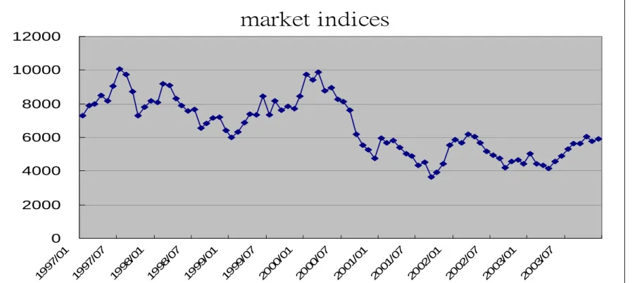
Our sample consists of all the TSE (Taiwan stock exchange) listed companies that have historical records of buys and sells and return data in the period January 1995 to December 2003. Figure 1 shows that Taiwan indices range from 10,000 to 4,000, experiencing bull and bear markets during the sample period.. Weekly and Monthly return series, risk free rate, book value of equity, closing prices and number of shares outstanding for a given stock, are from the Taiwan Economic Journal.

The order flow data are directly from the Taiwan stock exchange, enabling us to study investor behaviors directly.1 There are several advantages of our datasets. Firstly, unlike the

III41

1

(7)

ISSM and TAQ data sets, our order flow data contain whether an order was buy or sell initiated, which is very import for us to separate investors’ momentum/ contrarians in a pure way. Secondly, our dataset incorporates all of the orders entering the market and transactions, allowing us to use order flow information directly. The order information records all of the investors’ demands/supplies without any intervention of transaction rules if transaction data were adopted instead. Thirdly, the data provide an identification of all investors’ types (foreigners, domestic mutual funds, proprietary dealers, corporations and individuals), and furthermore, all of the account information that belong to one signal trader. This makes us to control for sophistication effect, which is well documented and inconclusive comparing foreign vs. domestic investors in the past studies.

All eligible buy or sell orders are aggregated based on all of the accounts for the same trader, and we assign an identification code for the same investors. Traders are then classified as either foreign individuals vs domestic individuals, foreign institutions vs domestic institutions, domestic big individuals or domestic small individuals. In Taiwan, foreign investors are foreign institutions mainly from the U.S. and Europe, while domestic institutions are mutual funds, proprietary dealers, and corporations. To further separating domestic individuals into big and small individuals, we set up the small-investor cut off points: traders were further classified as “large” if they submitted orders larger than ten lots more than 50% of the time over the entire sample period, and “small” otherwise.

We classify investors into two groups: domestic and foreign investors. Domestic investors include individual investors, corporate investors and domestic institutional investors. Foreign investors consist largely of international investment firms, primarily from the US and Europe. The tests are conduced based on the order flow data from the Taiwan Stock Exchange, covering the period of 1995 to 2003. This dataset has three key features that are crucial to our analysis. (i) It identifies whether an order is initiated by a buyer or a seller. (ii) The dataset also identifies the parties to the transaction (individual or institution). (iii) Our dataset enables us to trace all of the accounts that belong to one single trader, thus allows us to classify the cultural background of the investors.

Hypothesis

Three hypotheses are listed as below. By using the Taiwan stock market as the sample, we examine whether the momentum profits do exist in Taiwan. We take the momentum test and reverse it, and see if the opposite works. This study also examine whether or not stock momentum is shorter or longer in Taiwan than traditional US momentum for stocks.

(8)

Are there any systematic patterns of investors’ behaviors that account for momentum effect in Taiwan? We divide investors into foreign individuals vs. foreign institutions, domestic institutions vs domestic individuals, domestic big traders vs domestic small traders to test if the following hypothesis is supported.

Hypothesis 2: Chinese investors are contrarians, while foreign investors are momentum traders, supporting Yin-Yang theory.

How does order imbalance affects stock return? If there is no momentum, another follow- up question is that whether momentum effect is reduced by the trading behaviors from some types of investors. Particularly, we want to address who is taking the opposite side and eliminating momentum?

Hypothesis 3: Taiwanese investors take the opposite side and eliminating momentum.

III. Empirical Results

We capture the trading behavior of investors by the trade imbalance (buy minus sell) over a specific period of time (ranging from one week, one month to one year). For each investor group, we calculate the total order imbalance for every stock. Various tests are then conducted to see whether the trade imbalance is related with prior stock returns. To control for any difference in the level of sophistication between domestic and foreign investors, we further classify domestic investors into three sub-groups: institutional investor, big individual investor, and small individual investors.2 Lee, Lin and Liu (1999) documents systematic differences in investment behavior among these groups, and therefore, further tests are then conducted for each sub-groups of domestic investors.

Individual stock order imbalance is calculated as net buy ratio for stock i on day t. Net buy ratio (NBi, t) is the difference between all of the buy shares and sell shares in a group of investors

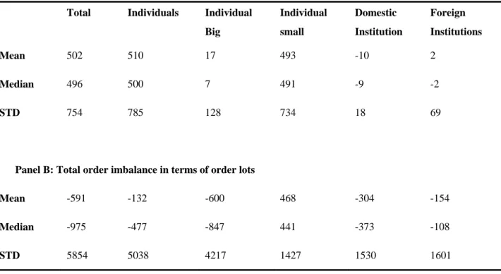
divided by the all of the buy and sell orders in the same group for stock i on day t. The buy /sell volume (in terms of shares and dollar amounts) is measured by each day and each stock for each type of investors mentioned above. We, then, summarize all of the variables for all types of investors throughout the sample period on a weekly and monthly basis in Table 1.

V41

2

(9)

[Please insert Table 1]

We, thus, report order imbalance in terms of number of orders (Panels A), order in lots (Panels B) in Table 1. The market are net buys (mean=502) in terms of number of orders, and net sellers in terms of order in lots (mean=-591). Since most of the trading volume is contributed by individuals, it is very natural to see that individual order imbalance follow a similar pattern. However, if we look at institutions, both domestic institutions and foreign institutions are net sellers during the sample period. Interestingly, small domestic investors are net buyers no matter what measurements are adopted.

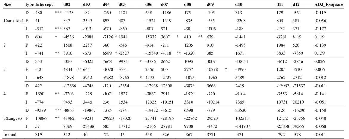
Furthermore, we look at order imbalance among 12 months, to investigate whether there is any systematic pattern for types of investors. For each month from 1995 to 2003, we categorize all stocks into five size deciles based on market capitalization at the end of the month t-2. We run regression models using 11 seasonal dummies (Feb. to Dec.) for each calendar month, and produce sixteen regressions. D, F, and I stands for domestic institutions, foreign institutions, and individuals, respectively. Meanwhile, the dependent variable is the monthly OIB in dollar amounts on portfolio p in month t. The dummy coefficients indicate the average differences in OIB between January and each respective month. The intercept is the average OIB for January. All of the coefficients are multiplied by 10,000.

From Table 2, we analyze order imbalance patterns, yet we do not see institutions moving into large stocks in December. Then, we see if institutions tend to sell losers and buy winners in December. We do this by regressing OIB on past returns*monthly dummy. We try different periods, 3, 6, 12 months and the results are shown We find that foreign institutions poss momentum for large firms (size group 4 and 5), Individual are basically contrarians, in particular for small firms (size group 1 and 2). Domestic institutions are momentums for small firms (size 1), yet contrarians for large firms (size 5). The phenomenon is partly because that domestic (foreign) institutions window dressing in small (large) firms, while individuals do not do so.

Following Jegadeesh and Titman (1993), we construct momentum portfolios as follows. Momentum strategies/returns are calculated by building up the combination (J, K) time interval, while J is one week, 1, 3, 6 to 12 months, respectively. We rank securities based on their past

J-week (month) performance (J = 1 week, 1, 3, 6 to 12 months) and evaluate the returns over the

(10)

ten deciles based on their past 1 week, 1, 3, 6, 12 months performances. The portfolio with the lowest (highest) past return is assigned as “Losers (Winners)”. In total, there is a combination (J,

K) of 4 * 4 *10 unrestricted momentum strategies. In addition, we also examine a second set of

160 strategies that skip a month (week) between the portfolio formation period and the holding period. The results are similar no matter when we skip a month (week) or not.

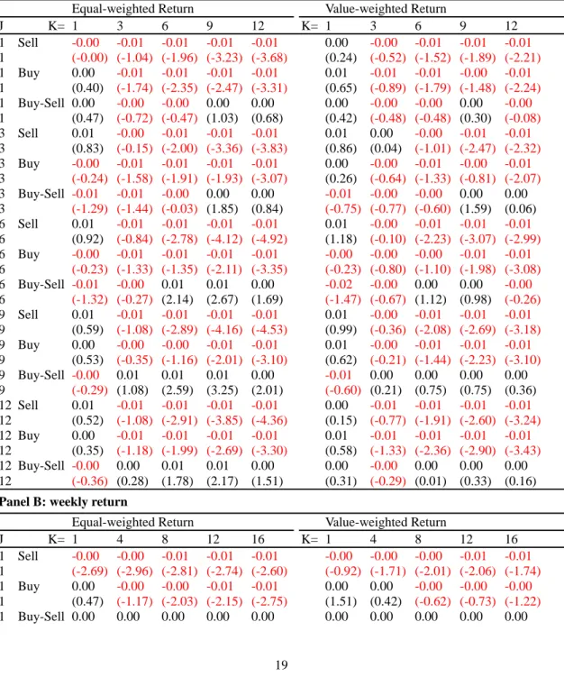
Table 3 reports the returns of relative strength portfolios. The relative strength portfolios are formed based on J-month lagged returns and held for K month. The values of J and K for the different strategies are indicated in the first column and row, respectively. The stocks are ranked in ascending order on the basis of J-month lagged returns and an equally weighted portfolio of the stocks in the lowest return decile is the sell portfolio and an equally weighted portfolio of the stocks in the highest return decile is the buy portfolio. The equally (value-) weighted average monthly returns of these portfolios are presented in this table.

In Table 3, Panel A, we reports is the results measured by monthly return, while Panel B is the results measured by weekly returns. Panel A, Table 3 indicates that most of the returns of all the zero-cost portfolios are negative. The returns are statistically significant for the 6-, 9- or 12-month holding periods, and insignificant for the 1- and 3-month strategy that skip a month. The return patterns are similar no matter when returns are measured by equal-weighted or value-weighted returns. If we look at weekly return, most of the returns for different holding period become more negative and statistically significant than monthly return. However, most of the results on value-weighted returns are not statistically significant. Negative returns do appear in some of the cases. In summary, we do not find momentum return in Taiwan.

Same as Table 3, momentum portfolios are constructed for types of investors, separately, in the same way as follows. At the end of each month, all stocks are ranked into 10 deciles based on their past 1 week, 1, 3, 6, 12 months. The portfolio with the lowest (highest) past return is assigned as “SELL (BUY)”. Then, we calculate net buys for different holding period to see if an investor tends to buy losers and sell winners (momentum). In the meantime, net buys are measured by equally (value-) weighted average monthly order imbalance (OIB) of these portfolios for all types of investors in terms of number of share and dollar amount. Results on number of shares are presented from Tables 3 to 6, respectively, for foreign individuals vs. domestic individuals (Table 3), foreign institutions vs. domestic institutions (Table 4) and domestic big investors vs. domestic small investors (Table 5). We report equally-weighted portfolio returns for different holding periods.

(11)

In Table 4, Panel A, we find that net buys are significantly positive in all strategies both for winners and losers. The results imply that the more extreme the past returns (winners or losers) are, the more likely that domestic individuals are going to buy it in the holding period. If we look at net buys of winners (Buy) minus net buys of losers (Sell) [Buy-Sell], the values are negative and statistically significant in all strategies, meaning that domestic individuals tend to buy more losers than winners. The phenomenon is consistent with contrarian trading strategy; that is domestic individuals trade against the market in the formation period.

The trading behaviors of foreign individuals are shown in Panel B, Table 4. Foreign individuals are net buyers when past returns are extremely negative or positive. However, the values of [Buy-Sell] are positive for all strategies, indicating that net buys of winners are greater than those of losers. Thus, foreign individuals are basically momentum traders over various formation period and holding periods. (1 week, 1 month, 3 month, 6 month, 1 year). The results of weekly net buys in Panels C and D are similar to those in Panels A and B, respectively.

In Table 5, we show results on domestic institutions and foreign institutions. Similarly, [Buy-Sell] of domestic institutions are negative, while that of foreign institutions are positive, implying that domestic (foreign) institutions are contrarian (momentum). When the magnitude of monthly [Buy-Sell] in Tables 3 and 4, we find that the values range from -0.01 to-0.02 for domestic individuals, 0.00 to 0.14 for foreign individuals, -0.02 to 0.00 for domestic institutions, and -0.01 to 0.19 for foreign institutions. The finding indicates the foreign investors tend to react to past returns significantly, while domestic investors only show slightly reaction on past return.

This paper further divides domestic individuals into big and small individuals, and the results on net buys are shown in Table 6. No matter what net buys of big or small individuals are considered, the finding is consistent with contrarian trading strategies for both of them. The monthly values of [Buy-Sell] for domestic big individuals are from 0.00 to -0.02, while those for domestic small ones are from -0.05 to -0.01. It is interesting to find that small domestic individuals tend to be more contrarian than big domestic individuals.

(12)

In Table 7, we examine whether order imbalance from any type of investors have impact on prices, to provide rationales on the sources of price momentums (contrarian), if any. We regress daily value-weighted returns (Rt.) on contemporaneous and lagged positive and negative daily

weighted order imbalances and past positive and negative value-weighted stock returns. Meanwhile, weighted order imbalances are value-weighted measured in number of orders and order in lots, respectively; EBO0 (EBO1) is the positive weighted order imbalance at day t (t-1)

and ESO0 (ESO1) is the negative weighted order imbalance; NEG (POS) indicates negative

(positive) lagged return.

According to Table 3, there is no price momentum in Taiwan, and Tables 4 and 5 shows that foreign (domestic) investors are momentum. It is an empirical question whether foreign (domestic) investors have positive (negative) impact on price. We expect to find that domestic investors contribute to more on price movement than foreign investors since there is no momentum profit in the market. Contrary to Hvidkjaer（2006）, we find that both Institutions (foreign and domestic) and bid traders have positive impact on stock prices significantly, while trades by domestic small investors have negative impact on prices. Since domestic investors (domestic institutions and big traders) seem to dominate the market, and their trade imbalance mostly determines the direction of stock movements. From Tables 3 to 5, foreign investors (institutions and individuals) are basically momentum and therefore, the price impact of such trading behavior is mitigated by the contrarian trading from domestic investors.

In summary, we find that no matter what weekly data or monthly data are used, Domestic Individuals adopt contrarian strategy. In contrast, foreign investors (including individuals, eastern institution, and western institution) adopt momentum strategy. The results are very similar to what we have obtained in earlier version. The results are similar no matter in terms of shares or amounts.

IV. Discussion and Conclusion

Our paper document momentum behaviors for both foreign institutiona and individuals. Domestic investors (including institutions and individuals, big and small traders) do not tend to

(13)

sluggish reaction to past returns, and they do have significant impact on moving prices in the same direction. Interestingly, foreign investors tend to react to past returns significantly, while domestic investors only show slightly reaction on past return. Besides, small domestic individuals tend to be more contrarian than big domestic individuals. Therefore, it is still a puzzle that whether psychology factors are the main rationales that explain momentum

This study builds on prior research in two fields: Psychology and Finance. Our study also contributes to the finance literature by exploring how cultural difference might affect individual’s investment decision and stock returns. In the behavioral finance studies several cognitive biases (e.g. self-attrition, conservatism, over-confidence) have been examined to provide explanation for certain observed stock market anomalies (Odean 1998; Daniel, Hirshleifer, and Subrahmanyam 1998, Jegadeesh and Titman 2001).

Jaggedness and Titman (2001) argue that the momentum effect is likely to be caused by the delayed over-reaction by investors. Such a theory, however, can not explain any difference in the magnitude of the momentum effect across countries. While Rouwenhorst (1998) document the momentum effect in 12 European countries, Liu and Lee (2001) shows that the phenomenon does not exist in Japan. Hameed and Kusnadi (2002) show that momentum investment strategies do not yield significant momentum profits in six Asian stock markets. Testing momentum effects in a sample of 9 Asian stock markets, Hou, McKnight, Gao (2005) find little evidence on the existence of intermediate stocks return continuation profits. The aforementioned evidences suggest that the factors that contribute to the momentum phenomenon in the United States are not prevalent in the Asian markets.

Though culture is influential in the financial decision-making process, behavioral finance has borrowed more from the cognitive psychology than from social psychology-culture. According to Chui, Titman and Wei (2003), a study by Hofstede (1991) found that people in Western countries tend to score higher in tests of “individualism” than do people in Asia. While it is not obvious how a tendency to think and act more or less independently relates to the momentum effect, it is quite plausible that individualism is related to “conservatism” and “overconfidence” which have been suggested by Barberis, Shleifer, and Vishny (BSV) (1998) and Daniel, Hirshleifer, and Subrahmanyam (DHS) (1998) as determinants of momentum.

One important principle underlying the dialectical lay theory is the principle of change, which argues that the universe is in a state of flux and that all objects, events, and states of being

(14)

in the world are forever alternating between two extremes or opposites (Yin and Yang).3 The principle of Yin-Yang has broad implications for human cognition, emotion, and behavior and affects the manner in which lay people in East Asian countries (notably, Japan, Korea, and China) deal with unfamiliar situations (Peng & Nisbett, 1999; Spencer-Rodgers & Peng, 2004). In the context of investment decisions, the lay theory of Yin-Yang would suggest that, conditional on observing good (or bad) past stock returns, such good (or bad) stock return are more likely to reverse than to continue in the future. We conjecture that Yin-Yang belief in the Asian culture may provide a potential explanation the observed foreign momentum/domestic contrarian phenomenon between the European and Asian markets.

XI41

3

For example, hot becomes cold, small becomes large, light becomes dark, love becomes hatred, and so on. Each element

(15)

Reference

Barberis, N., A. Shleifer, and R. Vishny, 1998, A model of investor sentiment, Journal of

Financial Economics, 49, 307-345.

Barclay, M. J., and J. B. Warner, 1993. Stealth trading and volatility: which trades. move prices? Journal of Financial Economics, 34, 281-305.

Chakravarty, S. 2001. Stealth-trading: Which traders' trades move stock prices? Journal of

Financial Economics, 61 (2): 289-307.

Chui, C.W.A., S. Titman, and K.C.J. Wei, 2003, Intra-industry momentum: the case of REITs, Journal of Financial Markets, Vol 6(3), 363-387.

Daniel, K.D., Hirshleifer, D., Subrahmanyam, A., 1998. Investor psychology and security market under- and over-reactions, Journal of Finance, 53, 1839-1886.

Fama, E. F. and K. R. French, 1996, Multifactor explanations of asset pricing. anomalies,

Journal of Finance, 51, 55-84.

Grinblatt M., and M. Keloharju, 2000, The investment behavior and performance of various investor types: A study of Finland’s unique data, Journal of Financial Economics, 55, 43-67.

Hameed A. and Y. Kusnadi, 2002, “Momentum strategies: Evidence from Pacific Basin stock markets,” The Journal of Financial Research, Vol. XXV, No. 3, Pages 383–397.

Hofstede, G. 1991, Cultures and organizations: Software of the mind, London. McGraw Hill.

Hvidljaer, S. (2006) A Trade-based analysis of momentum, Review of Financial Studies, V19, No. 2, 457-491.

Jegadeesh, N.and S. Titman 1993. Return to buying winner and selling losers: Implication for stock market efficiency. Journal of Finance, 48, 65-91.

Jegadeesh, N. and S. Titman 2001. Profitability of momentum strategy : A evaluation of alternative explanation. Journal of Finance, 56, 699-719.

Lee, Y., J. Lin, and Y. Liu 1999. Trading patterns of big versus small players in an emeerging market: An emepirical analysis. Journal of Banking and Finance, 23, 701-725.

Lee, M.C.C. and M.J. Ready, 1991, Inferring trade direction from intraday data, Journal

of Finance, 46, 733-746.

Liu, C., and Y. Lee, 2001, Does the momentum strategy work universally? Evidence from the Japanese Stock Market Asia-Pacific Financial Markets 8: 321–339.

(16)

1775-1798.

Peng, K., and R. E. Nisbett (1999) Culture, dialectics, and reasoning about contradiction. American Psychologist, 54, 741-754.

Rouwenhorst, G. (1998) International momentum strategies. Journal of Finance, 53(1), 267-284.

Spencer-Rodgers, J., & Peng, K. (2004). The diale ctical self: Contradiction, change, and holism in the East Asian self-concept. In R. M. Sorrentino, D. Times New Roman Cohen, J. M. Olsen, & M. P. Zanna (Eds.). Culture and social behavior: The Ontario symposium. Vol. 10, Mahwah, NJ: Lawrence Erlbaum.

(17)

market indices

0 2000 4000 6000 8000 10000 12000 1997 /01 1997 /07 1998 /01 1998 /07 1999 /01 1999 /07 2000 /01 2000 /07 2001 /01 2001 /07 2002 /01 2002 /07 2003 /01 2003 /07

(18)

Table 1 Order Imbalance

This study measures average daily weighted order imbalance from the TWSE (Taiwan Stock Exchange) over 1995 - 2003. Daily weighted order imbalance was calculated using total weighted buy orders minus total weighted selling orders. We separate total weighted order imbalance into the weighted imbalance of individual investors, domestic institutional investors and foreign investors. In addition, this paper divides the traders into big traders and small traders by tracing their order size during the sample period. A trader is classified as a big trader if he places an order greater than or equal to ten lots more than 50% of the time. In total, six kinds of traders’ types are classified. We calculate value-weighted order imbalance for thirty stocks for every day. This table presents weighted order imbalance in number of orders and order in lots, respectively. Panels A and B present the weighted order imbalance. Descriptive statistics are given for mean, median and standard deviation (STD) in each panel.

Panel A: Total order imbalance in terms of number of orders

Total Individuals Individual

Big Individual small Domestic Institution Foreign Institutions Mean 502 510 17 493 -10 2 Median 496 500 7 491 -9 -2 STD 754 785 128 734 18 69

Panel B: Total order imbalance in terms of order lots

Mean -591 -132 -600 468 -304 -154

Median -975 -477 -847 441 -373 -108

(19)

Table 2 Systematic Patterns in Order Imbalance

This table studies that whether there is a systematic pattern in order imbalance in January. For each month from 1995 to 2003, we categorize all stocks into five size deciles based on market capitalization at the end of the month t-2. We run regression models using 11 seasonal dummies (Feb. to Dec.) for each calendar month, and produce sixteen regressions. D, F, and I stands for domestic institutions, foreign institutions, and individuals, respectively. Meanwhile, the dependent variable is the monthly OIB in dollar amounts on portfolio p in month t. The dummy coefficients indicate the average differences in OIB between January and each respective month. The intercept is the average OIB for January. All of the coefficients are multiplied by 10,000.

Size type Intercept d02 d03 d04 d05 d06 d07 d08 d09 d10 d11 d12 ADJ_R-square

D 480 *** -1123 187 -260 1101 638 -1186 175 -705 313 179 -564 -0.119 F 41 847 2549 893 407 -1521 -1319 -835 -635 -2208 805 381 -0.056 1(smallest) I -512 *** 367 -913 -670 -860 -807 921 -30 1006 -188 -132 371 -0.177 D 604 * -4536 -2088 -7126 * 1948 15932 3607 * 410 ** 639 -1441 -3281 8119 0.119 F 422 1508 2287 360 -546 -914 -211 1205 910 -1498 1984 520 -0.139 2 I -741 ** 3910 -673 6589 * -2527 -15340 -4118 ** -1320 385 1671 3833 -7859 0.139 D 353 -350 -6325 7668 9975 * -3786 2662 1095 3007 -10054 -4612 -2846 0.026 F -12 4844 ** 644 -1078 -604 2356 500 2757 10778 * -4990 1205 3510 0.006 3 I -643 -1898 5952 -6282 -8965 * 4773 -2727 -1075 -1965 5489 2762 2712 -0.012 D 422 -12666 -4748 -1201 -2654 -12938 12308 -3873 9663 2419 -13962 -21532 -0.011 F 1690 ** -3203 1228 -1071 1527 -3867 2911 -1529 -720 -6104 -3553 -5814 -0.141 4 I -774 9493 3446 236 1534 12925 -10151 3310 -10214 7365 10731 20210 -0.051 D -9379 *** -8863 -19867 1375 -274 -19472 -4615 6598 -879 83530 6126 -16296 -0.150 F 10886 ** 41982 -9231 29923 -18020 27741 -28196 -22762 29523 102513 12152 -23758 -0.040 5(Largest) I 57 7369 28488 583 17712 -2166 27981 9708 -4472 -141937 -25858 39366 -0.068 In total 319 512 40 -72 -46 638 -326 -367 3771 -471 -792 -578 -0.011

(20)

Panel B: Past six-month return

Size type Intercept d02 d03 d04 d05 d06 d07 d08 d09 d10 d11 d12 ADJ_R-square

D 448 *** -1447 * -183 -51 1079 2947 * 630 -916 -633 -191 110 -448 0.007 F 22 1226 ** 4209 ** 811 246 -53 -968 -51 -74 -874 516 2117 0.078 1(smallest) I -487 *** 642 -563 -550 -786 -2968 * -926 791 1248 5 62 280 -0.063 D 218 1536 5215 1785 2616 * 16232 ** * 2071 ** 642 -557 -76 -2011 1683 0.121 F 456 -789 3446 197 -594 -2210 -193 933 483 -213 2758 5942 -0.087 2 I -445 -3971 -9407 ** -1192 -3005 ** -15493 ** * -2307 *** -930 1036 63 4597 -6640 0.250 D -118 -721 -3411 919 7525 ** 2801 3187 2589 2972 2824 -5030 2460 -0.023 F 69 3098 ** -384 -529 -724 48 -174 1045 2707 -3962 487 4822 -0.005 3 I -311 -480 3671 369 -6574 * -1449 -3060 -2499 -2485 -440 3889 -3618 -0.055 D -73 2298 -5940 -6156 -1574 -7246 6176 -849 4338 4407 -6842 -1639 -0.067 F 1566 ** -80 1875 796 1942 1738 -116 -452 -773 -7297 ** -1237 -9703 -0.021 4 I -78 -7848 1588 4759 1370 7744 -4145 188 -4790 1728 4961 1259 -0.102 D -8346 ** 20712 -5275 -4189 -2109 -28229 -2837 1041 133 18346 5943 -63688 ** -0.002 F 11625 *** -60583 29700 23948 -22002 3609 -12857 -16124 2671 4716 41074 23896 -0.061 5(Largest) I -733 9353 -6890 1685 14477 19993 13703 9674 1750 -17598 -40045 51271 -0.080 In total 295 -260 511 299 142 171 -141 -289 882 -210 12 1351 -0.012

(21)

Panel C: Past 12-month return

Size type Intercept d02 d03 d04 d05 d06 d07 d08 d09 d10 d11 d12 ADJ_R-square

D 568 *** -1229 * -661 289 952 2426 * 330 1165 606 691 -323 37 0.000 F 123 646 2568 *** 744 -252 250 -1171 75 359 -1311 -6 787 0.059 1(smallest) I -624 *** 683 -268 -781 -412 -2464 * -862 -625 -73 -629 391 -92 -0.074 D 636 * -3739 3660 2120 3838 ** -295 1412 21 740 1641 -4250 1121 0.052 F 389 2551 * 2477 ** 395 -928 -1363 -108 549 698 -2498 ** -1174 740 0.123 2 I -936 *** 221 -6548 ** -2239 -4111 ** -279 -1590 ** -382 -1346 -17 7704 -4725 0.175 D 205 -873 -5102 ** 1132 8043 * 1572 3623 * 1406 6390 * 1064 -13333 ** -134 0.137 F -112 3064 ** -412 -591 -515 -486 -345 1601 ** 230 -3946 *** -712 2317 * 0.141 3 I -552 -642 4935 ** -45 -5756 -216 -2865 -1834 -5449 -170 14265 ** -791 0.094 D 110 -4962 -7338 * -1310 -1766 -1429 3579 -578 3191 4734 ** -8077 * -1550 0.129 F 1635 ** -1916 960 484 -251 -863 -127 -82 -175 -2702 *** -1951 -1036 1 0.013 4 I -523 3236 5778 -81 2548 1560 -2271 85 -3623 -2064 8005 * 1441 0.004 D -5699 * -13034 -11586 * 356 -1624 -2937 5 ** -4273 -6694 -856 9746 -5670 -2486 9 ** * 0.109 F 15638 *** 31245 -8240 -21958 -20406 -2109 5 -15379 -1241 4 293 3945 8002 209 -0.045 5(Largest) I -5286 11117 16833 ** 11723 14648 42388 ** 16085 14940 2201 -10741 -2941 25049 ** 0.102 In total 323 570 -221 1 -319 -172 -57 -123 510 -254 394 359 -0.012

(22)

19

Table 3：Returns of Relative Strength Portfolios

The relative strength portfolios are formed based on -month lagged returns and held for K month. The values of J and K for the different strategies are indicated in the first column and row, respectively. The stocks are ranked in ascending order on the basis of J-month lagged returns and an equally weighted portfolio of the stocks in the lowest return decile is the sell portfolio and an equally weighted portfolio of the stocks in the highest return decile is the buy portfolio. The equally (value-) weighted average monthly returns of these portfolios are presented in this table. Panel A is results measured by monthly return, while panel B is the results measured by weekly returns. T-statistics are reported in parentheses.

Panel A: monthly return

Equal-weighted Return Value-weighted Return

J K= 1 3 6 9 12 K= 1 3 6 9 12 1 Sell -0.00 -0.01 -0.01 -0.01 -0.01 0.00 -0.00 -0.01 -0.01 -0.01 1 (-0.00) (-1.04) (-1.96) (-3.23) (-3.68) (0.24) (-0.52) (-1.52) (-1.89) (-2.21) 1 Buy 0.00 -0.01 -0.01 -0.01 -0.01 0.01 -0.01 -0.01 -0.00 -0.01 1 (0.40) (-1.74) (-2.35) (-2.47) (-3.31) (0.65) (-0.89) (-1.79) (-1.48) (-2.24) 1 Buy-Sell 0.00 -0.00 -0.00 0.00 0.00 0.00 -0.00 -0.00 0.00 -0.00 1 (0.47) (-0.72) (-0.47) (1.03) (0.68) (0.42) (-0.48) (-0.48) (0.30) (-0.08) 3 Sell 0.01 -0.00 -0.01 -0.01 -0.01 0.01 0.00 -0.00 -0.01 -0.01 3 (0.83) (-0.15) (-2.00) (-3.36) (-3.83) (0.86) (0.04) (-1.01) (-2.47) (-2.32) 3 Buy -0.00 -0.01 -0.01 -0.01 -0.01 0.00 -0.00 -0.01 -0.00 -0.01 3 (-0.24) (-1.58) (-1.91) (-1.93) (-3.07) (0.26) (-0.64) (-1.33) (-0.81) (-2.07) 3 Buy-Sell -0.01 -0.01 -0.00 0.00 0.00 -0.01 -0.00 -0.00 0.00 0.00 3 (-1.29) (-1.44) (-0.03) (1.85) (0.84) (-0.75) (-0.77) (-0.60) (1.59) (0.06) 6 Sell 0.01 -0.01 -0.01 -0.01 -0.01 0.01 -0.00 -0.01 -0.01 -0.01 6 (0.92) (-0.84) (-2.78) (-4.12) (-4.92) (1.18) (-0.10) (-2.23) (-3.07) (-2.99) 6 Buy -0.00 -0.01 -0.01 -0.01 -0.01 -0.00 -0.00 -0.00 -0.01 -0.01 6 (-0.23) (-1.33) (-1.35) (-2.11) (-3.35) (-0.23) (-0.80) (-1.10) (-1.98) (-3.08) 6 Buy-Sell -0.01 -0.00 0.01 0.01 0.00 -0.02 -0.00 0.00 0.00 -0.00 6 (-1.32) (-0.27) (2.14) (2.67) (1.69) (-1.47) (-0.67) (1.12) (0.98) (-0.26) 9 Sell 0.01 -0.01 -0.01 -0.01 -0.01 0.01 -0.00 -0.01 -0.01 -0.01 9 (0.59) (-1.08) (-2.89) (-4.16) (-4.53) (0.99) (-0.36) (-2.08) (-2.69) (-3.18) 9 Buy 0.00 -0.00 -0.00 -0.01 -0.01 0.01 -0.00 -0.01 -0.01 -0.01 9 (0.53) (-0.35) (-1.16) (-2.01) (-3.10) (0.62) (-0.21) (-1.44) (-2.23) (-3.10) 9 Buy-Sell -0.00 0.01 0.01 0.01 0.00 -0.01 0.00 0.00 0.00 0.00 9 (-0.29) (1.08) (2.59) (3.25) (2.01) (-0.60) (0.21) (0.75) (0.75) (0.36) 12 Sell 0.01 -0.01 -0.01 -0.01 -0.01 0.00 -0.01 -0.01 -0.01 -0.01 12 (0.52) (-1.08) (-2.91) (-3.85) (-4.36) (0.15) (-0.77) (-1.91) (-2.60) (-3.24) 12 Buy 0.00 -0.01 -0.01 -0.01 -0.01 0.01 -0.01 -0.01 -0.01 -0.01 12 (0.35) (-1.18) (-1.99) (-2.69) (-3.30) (0.58) (-1.33) (-2.36) (-2.90) (-3.43) 12 Buy-Sell -0.00 0.00 0.01 0.01 0.00 0.00 -0.00 0.00 0.00 0.00 12 (-0.36) (0.28) (1.78) (2.17) (1.51) (0.31) (-0.29) (0.01) (0.33) (0.16) Panel B: weekly return

Equal-weighted Return Value-weighted Return

J K= 1 4 8 12 16 K= 1 4 8 12 16 1 Sell -0.00 -0.00 -0.01 -0.01 -0.01 -0.00 -0.00 -0.00 -0.01 -0.01 1 (-2.69) (-2.96) (-2.81) (-2.74) (-2.60) (-0.92) (-1.71) (-2.01) (-2.06) (-1.74) 1 Buy 0.00 -0.00 -0.00 -0.01 -0.01 0.00 0.00 -0.00 -0.00 -0.00 1 (0.47) (-1.17) (-2.03) (-2.15) (-2.75) (1.51) (0.42) (-0.62) (-0.73) (-1.22) 1 Buy-Sell 0.00 0.00 0.00 0.00 0.00 0.00 0.00 0.00 0.00 0.00

(23)

1 (4.34) (2.78) (1.56) (1.31) (0.15) (2.66) (2.46) (1.68) (1.63) (0.71) 3 Sell -0.00 -0.00 -0.01 -0.01 -0.01 -0.00 -0.00 -0.00 -0.00 -0.01 3 (-2.25) (-2.08) (-2.45) (-2.26) (-2.27) (-1.47) (-1.06) (-1.91) (-1.86) (-1.72) 3 Buy -0.00 -0.00 -0.00 -0.01 -0.01 0.00 -0.00 -0.00 -0.00 -0.00 3 (-0.07) (-1.53) (-2.07) (-2.62) (-3.31) (0.82) (-0.29) (-0.25) (-0.52) (-1.36) 3 Buy-Sell 0.00 0.00 0.00 0.00 -0.00 0.00 0.00 0.00 0.00 0.00 3 (2.76) (0.91) (1.11) (0.09) (-0.96) (2.43) (0.86) (2.01) (1.71) (0.52) 6 Sell -0.00 -0.00 -0.01 -0.01 -0.01 -0.00 -0.00 -0.00 -0.00 -0.00 6 (-1.95) (-2.34) (-2.31) (-1.98) (-1.80) (-1.51) (-1.79) (-1.84) (-1.67) (-1.21) 6 Buy -0.00 -0.00 -0.00 -0.01 -0.01 -0.00 -0.00 -0.00 -0.00 -0.00 6 (-0.50) (-1.66) (-2.47) (-3.20) (-3.90) (-0.14) (-0.25) (-0.21) (-0.96) (-1.55) 6 Buy-Sell 0.00 0.00 0.00 -0.00 -0.00 0.00 0.00 0.00 0.00 -0.00 6 (1.85) (1.34) (0.61) (-0.88) (-2.02) (1.42) (1.78) (2.05) (1.06) (-0.17) 9 Sell -0.00 -0.00 -0.00 -0.00 -0.00 -0.00 -0.00 -0.00 -0.00 -0.00 9 (-1.87) (-1.76) (-1.71) (-1.23) (-1.14) (-1.19) (-1.07) (-1.32) (-1.05) (-1.25) 9 Buy -0.00 -0.00 -0.01 -0.01 -0.01 0.00 -0.00 -0.00 -0.00 -0.00 9 (-0.50) (-2.00) (-2.93) (-3.55) (-4.00) (0.48) (-0.04) (-0.68) (-1.28) (-1.64) 9 Buy-Sell 0.00 0.00 -0.00 -0.00 -0.01 0.00 0.00 0.00 -0.00 -0.00 9 (1.73) (0.23) (-0.80) (-2.14) (-2.79) (1.77) (1.17) (0.89) (-0.11) (-0.30) 12 Sell -0.00 -0.00 -0.00 -0.00 -0.00 -0.00 -0.00 0.00 -0.00 -0.00 12 (-1.34) (-1.33) (-0.84) (-0.59) (-0.72) (-0.65) (-0.41) (0.03) (-0.05) (-0.25) 12 Buy -0.00 -0.00 -0.01 -0.01 -0.01 0.00 -0.00 -0.00 -0.00 -0.01 12 (-0.82) (-2.41) (-3.26) (-3.75) (-4.04) (0.07) (-0.46) (-1.00) (-1.33) (-1.88) 12 Buy-Sell 0.00 -0.00 -0.00 -0.01 -0.01 0.00 0.00 -0.00 -0.00 -0.00 12 (0.76) (-0.74) (-2.15) (-2.99) (-3.30) (0.77) (0.01) (-1.05) (-1.26) (-1.65)

(24)

21

Table 4：Order Imbalance of Relative Strength Portfolios: Foreign Individuals vs. Domestic Individuals

The relative strength portfolios are formed based on J-month lagged returns and held for K month. The values of J and K for the different strategies are indicated in the first column and row, respectively. The stocks are ranked in ascending order on the basis of J-month lagged returns and an equally weighted portfolio of the stocks in the lowest return decile is the sell portfolio and an equally weighted portfolio of the stocks in the highest return decile is the buy portfolio. The equally (value-) weighted average monthly order imbalance (OIB) of these portfolios is presented in this table. We measure order imbalance (OIB) in terms of amount for all types of investors. Panel A (C) presents the results of domestic individuals on a monthly (weekly) basis, while Panel B (D) presents the results of foreign individuals on a monthly (weekly) basis. The t-statistics are reported in parentheses. The sample period is January 1995 to December 1999.

Panel A: domestic individuals (monthly)

Equal-weighted OIB Value-weighted OIB

J K= 1 3 6 9 12 K= 1 3 6 9 12 1 Sell 0.69 0.70 0.72 0.74 0.76 0.68 0.70 0.71 0.73 0.75 1 (24.26) (25.58) (27.90) (30.80) (34.60) (24.26) (25.58) (27.90) (30.80) (34.61) 1 Buy 0.68 0.69 0.71 0.73 0.75 0.67 0.69 0.71 0.73 0.75 1 (24.27) (25.58) (27.90) (30.81) (34.61) (24.26) (25.58) (27.90) (30.80) (34.61) 1 Buy-Sell -0.01 -0.01 -0.01 -0.01 -0.01 -0.01 -0.01 -0.01 -0.01 -0.00 1 (-7.55) (-7.59) (-6.86) (-6.21) (-5.85) (-5.95) (-6.01) (-5.05) (-4.38) (-3.78) 3 Sell 0.70 0.71 0.72 0.74 0.76 0.69 0.70 0.71 0.73 0.75 3 (24.26) (25.58) (27.90) (30.80) (34.60) (24.26) (25.58) (27.89) (30.80) (34.60) 3 Buy 0.68 0.69 0.71 0.73 0.75 0.67 0.69 0.71 0.72 0.74 3 (24.27) (25.58) (27.90) (30.80) (34.61) (24.27) (25.58) (27.90) (30.80) (34.61) 3 Buy-Sell -0.02 -0.01 -0.01 -0.01 -0.01 -0.01 -0.01 -0.01 -0.01 -0.01 3 (-9.50) (-9.22) (-8.69) (-8.07) (-7.33) (-7.32) (-7.38) (-6.79) (-6.57) (-5.96) 6 Sell 0.70 0.71 0.72 0.74 0.76 0.69 0.70 0.71 0.73 0.75 6 (24.26) (25.58) (27.90) (30.80) (34.61) (24.26) (25.58) (27.89) (30.80) (34.60) 6 Buy 0.68 0.69 0.71 0.73 0.75 0.67 0.69 0.71 0.72 0.74 6 (24.27) (25.58) (27.90) (30.80) (34.61) (24.27) (25.58) (27.90) (30.80) (34.60) 6 Buy-Sell -0.02 -0.02 -0.01 -0.01 -0.01 -0.01 -0.01 -0.01 -0.01 -0.01 6 (-11.70) (-11.24) (-10.10) (-9.73) (-9.11) (-8.19) (-8.07) (-7.52) (-7.30) (-6.42) 9 Sell 0.70 0.71 0.73 0.74 0.76 0.69 0.70 0.72 0.73 0.75 9 (24.26) (25.58) (27.90) (30.80) (34.61) (24.26) (25.58) (27.90) (30.80) (34.60) 9 Buy 0.68 0.69 0.71 0.73 0.75 0.67 0.69 0.71 0.72 0.74 9 (24.27) (25.58) (27.90) (30.80) (34.60) (24.27) (25.58) (27.90) (30.80) (34.61) 9 Buy-Sell -0.02 -0.02 -0.01 -0.01 -0.01 -0.01 -0.01 -0.01 -0.01 -0.01 9 (-12.73) (-11.95) (-11.48) (-11.33) (-11.42) (-8.87) (-8.94) (-8.88) (-8.64) (-8.14) 12 Sell 0.70 0.71 0.73 0.74 0.76 0.69 0.70 0.72 0.74 0.75 12 (24.26) (25.58) (27.90) (30.80) (34.61) (24.26) (25.57) (27.89) (30.79) (34.60) 12 Buy 0.68 0.69 0.71 0.73 0.75 0.67 0.69 0.71 0.72 0.74 12 (24.27) (25.58) (27.90) (30.80) (34.61) (24.27) (25.58) (27.90) (30.80) (34.61)

(25)

12 Buy-Sell -0.02 -0.02 -0.02 -0.01 -0.01 -0.02 -0.01 -0.01 -0.01 -0.01

12 -12.08 -11.88 -11.9 -12.29 -11.97 -8.797 -8.711 -8.573 -8.305 -7.889

Panel B: foreign individuals (monthly)

J K= 1 3 6 9 12 K= 1 3 6 9 12 1 Sell 0.24 0.35 0.42 0.47 0.51 0.43 0.51 0.56 0.59 0.62 1 (13.76) (15.60) (17.03) (17.85) (19.18) (15.72) (17.20) (18.82) (19.64) (21.26) 1 Buy 0.30 0.39 0.45 0.50 0.53 0.47 0.52 0.56 0.60 0.62 1 (14.37) (16.11) (17.13) (18.83) (19.89) (15.91) (17.37) (18.25) (20.19) (21.44) 1 Buy-Sell 0.06 0.04 0.02 0.03 0.02 0.03 0.01 0.00 0.01 -0.00 1 (3.84) (3.04) (2.02) (3.08) (1.80) (2.06) (1.29) (0.02) (0.84) (-0.31) 3 Sell 0.23 0.34 0.42 0.47 0.51 0.42 0.50 0.55 0.59 0.62 3 (13.87) (15.51) (16.87) (17.72) (18.95) (15.18) (17.41) (18.54) (19.54) (21.03) 3 Buy 0.31 0.40 0.46 0.51 0.54 0.47 0.53 0.56 0.60 0.62 3 (14.66) (16.17) (17.29) (19.03) (20.18) (16.07) (17.35) (18.34) (20.42) (21.68) 3 Buy-Sell 0.08 0.06 0.05 0.04 0.03 0.05 0.03 0.01 0.01 0.01 3 (4.78) (4.40) (3.60) (3.28) (2.41) (2.40) (2.03) (0.89) (1.27) (0.87) 6 Sell 0.24 0.35 0.42 0.47 0.51 0.43 0.52 0.56 0.58 0.62 6 (14.09) (15.77) (16.79) (17.81) (19.15) (15.72) (17.56) (18.42) (19.45) (21.04) 6 Buy 0.33 0.41 0.48 0.52 0.55 0.48 0.53 0.58 0.60 0.62 6 (14.64) (16.14) (17.79) (19.12) (19.92) (16.05) (17.22) (19.02) (20.55) (21.65) 6 Buy-Sell 0.09 0.07 0.06 0.05 0.03 0.05 0.02 0.02 0.02 0.00 6 (5.38) (5.10) (4.96) (4.51) (3.33) (2.52) (1.35) (1.45) (1.77) (0.13) 9 Sell 0.22 0.34 0.42 0.47 0.52 0.41 0.51 0.55 0.58 0.62 9 (13.78) (15.54) (16.82) (17.90) (19.29) (15.23) (17.16) (18.24) (19.40) (20.89) 9 Buy 0.34 0.43 0.49 0.52 0.55 0.49 0.55 0.59 0.61 0.62 9 (15.00) (16.71) (18.02) (19.02) (20.09) (16.52) (18.01) (19.29) (20.52) (21.57) 9 Buy-Sell 0.12 0.09 0.07 0.05 0.04 0.08 0.05 0.04 0.03 0.01 9 (7.51) (7.12) (6.47) (5.41) (4.19) (4.26) (3.76) (3.60) (3.05) (0.75) 12 Sell 0.21 0.32 0.40 0.46 0.50 0.39 0.48 0.53 0.57 0.60 12 (14.10) (15.57) (16.60) (17.74) (18.65) (15.18) (17.00) (18.11) (19.43) (20.38) 12 Buy 0.35 0.43 0.49 0.53 0.56 0.51 0.55 0.58 0.60 0.62 12 (15.12) (16.48) (17.61) (18.85) (20.15) (17.06) (17.96) (19.07) (20.14) (21.58) 12 Buy-Sell 0.14 0.11 0.09 0.07 0.06 0.12 0.08 0.05 0.03 0.02 12 (8.09) (7.58) (6.91) (5.95) (5.08) (6.22) (5.69) (4.61) (2.96) (2.34)

Panel C: domestic individuals (weekly)

J K= 1 4 8 12 16 K= 1 4 8 12 16 1 Sell 0.69 0.70 0.70 0.71 0.71 0.68 0.69 0.69 0.70 0.70 1 (51.13) (52.08) (53.38) (54.76) (56.23) (51.12) (52.07) (53.38) (54.75) (56.22) 1 Buy 0.69 0.69 0.70 0.70 0.71 0.68 0.68 0.69 0.69 0.70 1 (51.14) (52.09) (53.39) (54.77) (56.23) (51.13) (52.08) (53.38) (54.76) (56.22) 1 Buy-Sell -0.01 -0.01 -0.01 -0.01 -0.01 -0.01 -0.01 -0.01 -0.00 -0.00 1 (-11.64)(-11.17) (-10.42) (-9.96) (-9.18) (-7.27) (-7.65) (-7.87) (-7.31) (-6.62)

(26)

23 4 Sell 0.70 0.70 0.70 0.71 0.71 0.69 0.69 0.70 0.70 0.71 4 (51.13) (52.08) (53.38) (54.76) (56.22) (51.12) (52.07) (53.38) (54.75) (56.22) 4 Buy 0.68 0.69 0.69 0.70 0.70 0.68 0.68 0.69 0.69 0.70 4 (51.14) (52.09) (53.39) (54.77) (56.23) (51.13) (52.08) (53.38) (54.76) (56.22) 4 Buy-Sell -0.02 -0.01 -0.01 -0.01 -0.01 -0.01 -0.01 -0.01 -0.01 -0.01 4 (-18.75)(-19.80) (-17.50) (-17.19) (-15.68) (-13.26) (-14.93) (-13.97)(-13.38)(-12.17) 8 Sell 0.70 0.70 0.71 0.71 0.72 0.69 0.69 0.70 0.70 0.71 8 (51.13) (52.08) (53.38) (54.76) (56.22) (51.11) (52.07) (53.38) (54.76) (56.22) 8 Buy 0.68 0.69 0.69 0.70 0.70 0.67 0.68 0.68 0.69 0.70 8 (51.14) (52.09) (53.39) (54.77) (56.23) (51.13) (52.09) (53.39) (54.76) (56.23) 8 Buy-Sell -0.02 -0.02 -0.02 -0.01 -0.01 -0.01 -0.01 -0.01 -0.01 -0.01 8 (-19.97)(-21.38) (-20.56) (-19.64) (-18.67) (-15.08) (-17.79) (-17.75)(-16.71)(-15.35) 12 Sell 0.70 0.70 0.71 0.71 0.72 0.69 0.69 0.70 0.70 0.71 12 (51.12) (52.07) (53.38) (54.76) (56.22) (51.12) (52.07) (53.38) (54.76) (56.22) 12 Buy 0.68 0.68 0.69 0.70 0.70 0.67 0.68 0.68 0.69 0.70 12 (51.15) (52.09) (53.39) (54.77) (56.23) (51.14) (52.09) (53.39) (54.77) (56.23) 12 Buy-Sell -0.02 -0.02 -0.02 -0.02 -0.01 -0.02 -0.02 -0.01 -0.01 -0.01 12 (-22.48)(-24.00) (-22.47) (-22.15) (-21.41) (-17.99) (-20.19) (-19.46)(-18.51)(-17.56) 16 Sell 0.70 0.70 0.71 0.71 0.72 0.69 0.69 0.70 0.70 0.71 16 (51.13) (52.07) (53.38) (54.76) (56.22) (51.11) (52.07) (53.37) (54.75) (56.22) 16 Buy 0.68 0.68 0.69 0.70 0.70 0.67 0.68 0.68 0.69 0.70 16 (51.15) (52.09) (53.39) (54.77) (56.23) (51.14) (52.08) (53.39) (54.77) (56.23) 16 Buy-Sell -0.02 -0.02 -0.02 -0.02 -0.01 -0.02 -0.02 -0.01 -0.01 -0.01 16 (-22.98)(-23.63) (-22.94) (-22.73) (-22.05) (-17.57) (-18.86) (-18.23)(-17.81)(-17.36)

Panel D: foreign individuals (weekly)

J K= 1 4 8 12 16 K= 1 4 8 12 16 1 Sell 0.15 0.25 0.31 0.35 0.38 0.34 0.45 0.49 0.52 0.53 1 (25.67) (29.83) (31.56) (32.94) (33.92) (27.13) (33.02) (34.98) (36.16) (37.25) 1 Buy 0.18 0.28 0.34 0.37 0.40 0.36 0.45 0.50 0.52 0.54 1 (26.46) (30.70) (32.59) (33.82) (34.91) (28.16) (33.37) (35.27) (36.52) (37.47) 1 Buy-Sell 0.03 0.03 0.02 0.02 0.02 0.02 0.01 0.00 0.00 0.00 1 (4.69) (4.00) (3.39) (3.59) (3.48) (1.86) (0.87) (0.55) (0.75) (0.45) 4 Sell 0.14 0.24 0.30 0.34 0.37 0.33 0.44 0.48 0.50 0.52 4 (25.72) (29.64) (31.10) (32.41) (33.56) (27.41) (32.94) (34.67) (35.91) (36.91) 4 Buy 0.19 0.29 0.35 0.39 0.41 0.37 0.46 0.50 0.53 0.54 4 (25.66) (30.75) (32.89) (34.27) (35.07) (28.73) (33.85) (35.64) (36.71) (37.50) 4 Buy-Sell 0.05 0.05 0.05 0.05 0.04 0.04 0.03 0.03 0.02 0.01 4 (7.33) (7.16) (7.36) (7.09) (6.57) (4.06) (3.31) (3.44) (3.26) (2.37) 8 Sell 0.13 0.23 0.29 0.33 0.37 0.31 0.42 0.47 0.50 0.52 8 (25.23) (29.20) (31.06) (32.55) (33.77) (26.25) (32.19) (34.44) (35.87) (36.91) 8 Buy 0.20 0.31 0.37 0.40 0.42 0.37 0.47 0.51 0.53 0.54 8 (26.24) (31.12) (33.40) (34.43) (35.05) (28.76) (33.76) (35.95) (36.79) (37.51) 8 Buy-Sell 0.06 0.08 0.07 0.06 0.05 0.06 0.05 0.04 0.03 0.02

(27)

8 (9.46) (10.23) (10.18) (9.20) (7.98) (4.99) (5.31) (5.58) (4.00) (3.51) 12 Sell 0.13 0.23 0.29 0.33 0.37 0.31 0.42 0.47 0.50 0.52 12 (25.22) (29.07) (31.20) (32.65) (33.84) (25.78) (31.79) (34.50) (36.15) (37.34) 12 Buy 0.20 0.31 0.37 0.40 0.43 0.38 0.47 0.51 0.53 0.55 12 (26.48) (31.44) (33.44) (34.44) (35.06) (29.07) (34.26) (36.02) (37.03) (37.59) 12 Buy-Sell 0.07 0.09 0.08 0.07 0.06 0.07 0.06 0.04 0.03 0.03 12 (10.55) (11.35) (10.74) (9.64) (8.90) (5.99) (5.99) (5.00) (4.20) (4.12) 16 Sell 0.13 0.23 0.29 0.33 0.37 0.31 0.42 0.47 0.50 0.52 16 (25.30) (28.81) (30.95) (32.50) (33.90) (25.89) (31.61) (34.49) (36.31) (37.56) 16 Buy 0.20 0.31 0.37 0.41 0.43 0.38 0.47 0.51 0.53 0.55 16 (26.34) (31.21) (33.32) (34.26) (35.09) (28.82) (33.99) (35.99) (36.74) (37.59) 16 Buy-Sell 0.07 0.08 0.08 0.07 0.06 0.07 0.05 0.04 0.03 0.03 16 (10.54) (10.99) (10.67) (9.92) (9.30) (5.54) (5.41) (5.40) (4.76) (4.28)

(28)

25

Table 5：Order Imbalance of Relative Strength Portfolios: Domestic Institutions vs. Foreign Institutions

The relative strength portfolios are formed based on J-month lagged returns and held for K month. The values of J and K for the different strategies are indicated in the first column and row, respectively. The stocks are ranked in ascending order on the basis of J-month lagged returns and an equally weighted portfolio of the stocks in the lowest return decile is the sell portfolio and an equally weighted portfolio of the stocks in the highest return decile is the buy portfolio. The equally (value-) weighted average monthly order imbalance (OIB) of these portfolios is presented in this table. We measure order imbalance (OIB) in terms of amount for all types of investors. Panel A (C) presents the results of domestic institutions on a monthly (weekly) basis, while Panel B (D) presents the results of foreign institutions on a monthly (weekly) basis. The t-statistics are reported in parentheses. The sample period is January 1995 to December 1999. ]

Panel A: domestic institutions (monthly)

J K= 1 3 6 9 12 K= 1 3 6 9 12 1 Sell 0.70 0.72 0.74 0.76 0.78 0.70 0.71 0.73 0.75 0.77 1 (24.19) (25.55) (27.87) (30.77) (34.57) (24.21) (25.55) (27.85) (30.75) (34.54) 1 Buy 0.70 0.71 0.73 0.75 0.77 0.69 0.70 0.72 0.75 0.76 1 (24.20) (25.56) (27.88) (30.78) (34.58) (24.20) (25.55) (27.87) (30.77) (34.57) 1 Buy-Sell -0.01 -0.01 -0.01 -0.01 -0.01 -0.01 -0.01 -0.00 -0.00 -0.00 1 (-2.32) (-3.82) (-3.36) (-3.05) (-2.88) (-2.85) (-3.02) (-1.95) (-1.16) (-1.74) 3 Sell 0.70 0.72 0.74 0.76 0.78 0.70 0.71 0.73 0.75 0.77 3 (24.19) (25.54) (27.87) (30.76) (34.56) (24.21) (25.54) (27.84) (30.74) (34.54) 3 Buy 0.70 0.71 0.73 0.75 0.77 0.69 0.70 0.72 0.75 0.76 3 (24.22) (25.56) (27.87) (30.77) (34.56) (24.20) (25.54) (27.87) (30.77) (34.57) 3 Buy-Sell -0.01 -0.01 -0.01 -0.01 -0.01 -0.01 -0.01 -0.01 -0.00 -0.01 3 (-1.92) (-4.10) (-4.31) (-3.83) (-4.16) (-3.11) (-3.02) (-2.30) (-1.53) (-2.65) 6 Sell 0.70 0.72 0.74 0.76 0.78 0.70 0.71 0.73 0.75 0.77 6 (24.19) (25.54) (27.86) (30.76) (34.56) (24.21) (25.53) (27.84) (30.76) (34.55) 6 Buy 0.70 0.71 0.73 0.75 0.77 0.69 0.70 0.72 0.74 0.76 6 (24.22) (25.56) (27.88) (30.77) (34.57) (24.22) (25.56) (27.88) (30.78) (34.58) 6 Buy-Sell -0.01 -0.01 -0.01 -0.01 -0.01 -0.01 -0.01 -0.01 -0.01 -0.01 6 (-1.71) (-4.53) (-5.30) (-5.75) (-5.71) (-4.50) (-3.56) (-2.61) (-4.14) (-5.28) 9 Sell 0.71 0.72 0.74 0.76 0.78 0.70 0.71 0.73 0.75 0.77 9 (24.19) (25.53) (27.86) (30.76) (34.56) (24.18) (25.51) (27.84) (30.75) (34.54) 9 Buy 0.69 0.71 0.73 0.75 0.77 0.69 0.70 0.72 0.74 0.76 9 (24.22) (25.56) (27.87) (30.77) (34.57) (24.22) (25.56) (27.88) (30.78) (34.59) 9 Buy-Sell -0.01 -0.01 -0.01 -0.01 -0.01 -0.01 -0.01 -0.01 -0.01 -0.01 9 (-3.76) (-6.12) (-6.81) (-7.24) (-6.62) (-4.35) (-3.60) (-3.87) (-5.24) (-5.62) 12 Sell 0.71 0.72 0.74 0.76 0.78 0.71 0.72 0.73 0.75 0.77 12 (24.17) (25.54) (27.86) (30.76) (34.55) (24.20) (25.52) (27.84) (30.74) (34.51) 12 Buy 0.70 0.71 0.73 0.74 0.76 0.69 0.70 0.72 0.74 0.76 12 (24.23) (25.55) (27.87) (30.78) (34.57) (24.23) (25.56) (27.88) (30.79) (34.59)

(29)

12 Buy-Sell -0.01 -0.02 -0.02 -0.02 -0.01 -0.01 -0.01 -0.01 -0.01 -0.01 12 (-2.93) (-6.34) (-7.87) (-7.71) (-6.71) (-5.23) (-5.13) (-5.11) (-4.89) (-4.83) Panel B: foreign institutions (monthly)

J K= 1 3 6 9 12 K= 1 3 6 9 12 1 Sell 0.44 0.57 0.65 0.69 0.73 0.63 0.68 0.71 0.74 0.76 1 (20.41) (23.68) (26.74) (29.78) (33.58) (23.39) (25.28) (27.71) (30.60) (34.35) 1 Buy 0.53 0.62 0.67 0.71 0.74 0.66 0.69 0.72 0.74 0.76 1 (22.01) (24.22) (27.01) (30.07) (33.89) (23.80) (25.28) (27.67) (30.63) (34.48) 1 Buy-Sell 0.08 0.05 0.02 0.02 0.01 0.03 0.01 0.00 0.00 0.00 1 (6.13) (4.33) (3.19) (2.55) (1.72) (3.95) (2.61) (0.56) (0.51) (0.34) 3 Sell 0.43 0.57 0.65 0.70 0.73 0.61 0.67 0.71 0.74 0.76 3 (20.49) (23.70) (26.60) (29.79) (33.39) (22.84) (25.06) (27.56) (30.55) (34.32) 3 Buy 0.55 0.63 0.68 0.72 0.74 0.67 0.70 0.72 0.74 0.76 3 (22.24) (24.48) (27.15) (30.16) (33.95) (23.76) (25.31) (27.74) (30.62) (34.45) 3 Buy-Sell 0.12 0.06 0.04 0.02 0.01 0.05 0.02 0.01 0.00 0.00 3 (8.09) (6.34) (4.70) (2.89) (1.63) (4.50) (3.40) (1.97) (0.91) (0.13) 6 Sell 0.42 0.56 0.65 0.70 0.73 0.62 0.68 0.72 0.75 0.77 6 (20.09) (23.76) (26.61) (29.62) (33.28) (23.09) (25.18) (27.60) (30.50) (34.31) 6 Buy 0.57 0.65 0.69 0.72 0.75 0.68 0.70 0.72 0.74 0.76 6 (22.97) (24.94) (27.36) (30.38) (34.17) (24.01) (25.47) (27.82) (30.74) (34.51) 6 Buy-Sell 0.15 0.08 0.04 0.02 0.01 0.06 0.02 0.00 -0.00 -0.01 6 (10.96) (9.29) (5.23) (3.22) (2.27) (6.21) (3.85) (0.58) (-1.24) (-2.07) 9 Sell 0.41 0.56 0.65 0.70 0.74 0.60 0.68 0.72 0.75 0.77 9 (20.19) (23.79) (26.55) (29.51) (33.37) (22.70) (25.12) (27.59) (30.53) (34.37) 9 Buy 0.59 0.66 0.70 0.73 0.75 0.68 0.70 0.73 0.75 0.77 9 (23.01) (24.90) (27.45) (30.49) (34.26) (24.09) (25.48) (27.83) (30.76) (34.56) 9 Buy-Sell 0.18 0.09 0.05 0.03 0.01 0.08 0.02 0.00 -0.00 -0.00 9 (13.17) (9.88) (6.48) (4.46) (2.46) (7.64) (4.10) (1.03) (-0.61) (-1.46) 12 Sell 0.41 0.55 0.64 0.69 0.73 0.60 0.68 0.72 0.75 0.77 12 (20.08) (23.42) (26.17) (29.34) (33.25) (22.72) (25.17) (27.60) (30.56) (34.35) 12 Buy 0.60 0.66 0.70 0.73 0.75 0.68 0.70 0.73 0.75 0.77 12 (23.15) (25.04) (27.58) (30.56) (34.38) (24.07) (25.51) (27.87) (30.77) (34.56) 12 Buy-Sell 0.19 0.10 0.06 0.04 0.02 0.08 0.02 0.01 -0.00 -0.01 12 (13.26) (10.34) (7.58) (5.37) (3.66) (7.55) (4.41) (1.41) (-0.29) (-1.93)

Panel C: domestic institutions (weekly)

J K= 1 4 8 12 16 K= 1 4 8 12 16 1 Sell 0.68 0.71 0.72 0.72 0.73 0.70 0.70 0.71 0.71 0.72 1 (50.53) (51.94) (53.28) (54.67) (56.14) (50.86) (51.94) (53.28) (54.68) (56.15) 1 Buy 0.68 0.70 0.71 0.72 0.72 0.70 0.70 0.71 0.71 0.72 1 (50.69) (51.95) (53.28) (54.68) (56.15) (50.88) (51.96) (53.29) (54.68) (56.15) 1 Buy-Sell 0.01 -0.00 -0.00 -0.00 -0.00 0.00 -0.00 -0.00 -0.00 -0.00 1 (3.81) (-1.63) (-3.55) (-3.21) (-3.67) (0.44) (-0.69) (-1.90) (-2.63) (-3.27)

(30)

27 4 Sell 0.68 0.71 0.72 0.72 0.73 0.70 0.71 0.71 0.72 0.72 4 (50.42) (51.94) (53.28) (54.68) (56.14) (50.83) (51.95) (53.29) (54.69) (56.15) 4 Buy 0.69 0.70 0.71 0.72 0.72 0.70 0.70 0.70 0.71 0.71 4 (50.76) (51.96) (53.29) (54.68) (56.15) (50.90) (51.95) (53.29) (54.68) (56.15) 4 Buy-Sell 0.01 -0.01 -0.01 -0.01 -0.01 -0.00 -0.01 -0.01 -0.01 -0.01 4 (4.10) (-5.68) (-7.76) (-8.15) (-8.64) (-2.04) (-5.16) (-6.67) (-6.91) (-7.19) 8 Sell 0.68 0.71 0.72 0.73 0.73 0.70 0.71 0.71 0.72 0.72 8 (50.34) (51.94) (53.29) (54.68) (56.15) (50.76) (51.93) (53.28) (54.67) (56.13) 8 Buy 0.69 0.70 0.71 0.71 0.72 0.70 0.70 0.70 0.71 0.71 8 (50.83) (51.96) (53.30) (54.69) (56.16) (50.90) (51.95) (53.30) (54.69) (56.16) 8 Buy-Sell 0.01 -0.01 -0.01 -0.01 -0.01 -0.00 -0.01 -0.01 -0.01 -0.01 8 (4.66) (-7.27) (-9.59) (-10.52) (-9.45) (-2.02) (-6.00) (-6.91) (-7.56) (-6.83) 12 Sell 0.68 0.71 0.72 0.72 0.73 0.70 0.71 0.71 0.72 0.72 12 (50.34) (51.92) (53.28) (54.67) (56.14) (50.78) (51.95) (53.29) (54.67) (56.14) 12 Buy 0.69 0.70 0.71 0.71 0.72 0.70 0.70 0.70 0.71 0.71 12 (50.88) (51.97) (53.31) (54.70) (56.17) (50.90) (51.96) (53.30) (54.68) (56.16) 12 Buy-Sell 0.01 -0.01 -0.01 -0.01 -0.01 -0.01 -0.01 -0.01 -0.01 -0.01 12 (5.11) (-5.94) (-9.29) (-10.57) (-9.79) (-3.24) (-6.65) (-7.61) (-8.17) (-7.18) 16 Sell 0.68 0.71 0.72 0.73 0.73 0.70 0.71 0.71 0.72 0.72 16 (50.32) (51.92) (53.28) (54.67) (56.15) (50.81) (51.93) (53.28) (54.67) (56.14) 16 Buy 0.69 0.70 0.71 0.71 0.72 0.70 0.70 0.70 0.71 0.71 16 (50.90) (51.99) (53.32) (54.71) (56.17) (50.91) (51.96) (53.29) (54.68) (56.16) 16 Buy-Sell 0.01 -0.01 -0.01 -0.01 -0.01 -0.01 -0.01 -0.01 -0.01 -0.01 16 (5.46) (-6.33) (-10.04) (-11.02) (-10.30) (-4.55) (-8.21) (-9.03) (-9.17) (-7.57)

Panel D: foreign institutions (weekly)

J K= 1 4 8 12 16 K= 1 4 8 12 16 1 Sell 0.33 0.46 0.53 0.58 0.61 0.57 0.63 0.67 0.69 0.70 1 (39.03) (44.45) (47.85) (50.31) (52.56) (45.10) (49.74) (52.17) (53.93) (55.61) 1 Buy 0.38 0.50 0.57 0.60 0.63 0.59 0.65 0.68 0.69 0.70 1 (40.41) (46.02) (49.06) (51.27) (53.21) (46.40) (50.27) (52.32) (53.98) (55.54) 1 Buy-Sell 0.04 0.04 0.03 0.02 0.02 0.02 0.02 0.01 0.01 0.00 1 (5.93) (6.60) (6.11) (5.14) (5.00) (2.81) (3.52) (3.20) (2.68) (1.79) 4 Sell 0.32 0.45 0.52 0.57 0.61 0.56 0.63 0.66 0.68 0.70 4 (37.98) (43.27) (47.28) (50.35) (52.63) (45.10) (49.37) (52.02) (53.84) (55.45) 4 Buy 0.40 0.53 0.59 0.62 0.64 0.60 0.66 0.69 0.70 0.71 4 (41.11) (46.67) (49.78) (51.82) (53.79) (46.39) (50.50) (52.63) (54.21) (55.74) 4 Buy-Sell 0.08 0.07 0.06 0.05 0.04 0.04 0.03 0.02 0.02 0.01 4 (10.12) (10.56) (11.04) (9.81) (8.98) (5.38) (6.32) (6.97) (6.41) (5.37) 8 Sell 0.31 0.44 0.52 0.57 0.60 0.55 0.62 0.66 0.68 0.69 8 (37.02) (43.24) (47.25) (50.13) (52.48) (44.00) (49.08) (51.98) (53.73) (55.34) 8 Buy 0.42 0.54 0.59 0.63 0.65 0.61 0.67 0.69 0.70 0.71 8 (42.67) (47.27) (49.82) (51.95) (53.93) (47.56) (50.79) (52.68) (54.25) (55.80) 8 Buy-Sell 0.11 0.10 0.08 0.06 0.05 0.07 0.05 0.03 0.02 0.02

(31)

8 (13.25) (13.63) (12.75) (11.62) (10.54) (7.67) (8.57) (9.06) (8.38) (7.06) 12 Sell 0.31 0.44 0.52 0.57 0.60 0.54 0.62 0.66 0.68 0.69 12 (37.36) (43.28) (47.39) (50.17) (52.54) (44.20) (49.37) (52.08) (53.74) (55.41) 12 Buy 0.43 0.55 0.60 0.63 0.65 0.62 0.67 0.69 0.70 0.71 12 (42.78) (47.37) (50.04) (52.20) (54.10) (47.87) (50.91) (52.71) (54.23) (55.75) 12 Buy-Sell 0.13 0.11 0.09 0.07 0.05 0.08 0.05 0.04 0.03 0.02 12 (15.20) (15.49) (14.65) (13.55) (12.11) (8.99) (9.68) (9.68) (8.47) (6.83) 16 Sell 0.30 0.43 0.51 0.56 0.60 0.54 0.62 0.66 0.68 0.70 16 (36.69) (43.25) (47.33) (50.36) (52.71) (43.85) (49.46) (51.94) (53.84) (55.50) 16 Buy 0.44 0.56 0.61 0.64 0.66 0.62 0.67 0.69 0.70 0.71 16 (42.90) (47.71) (50.26) (52.37) (54.28) (47.57) (50.89) (52.60) (54.20) (55.76) 16 Buy-Sell 0.14 0.12 0.10 0.07 0.06 0.09 0.05 0.04 0.02 0.01 16 (16.92) (17.00) (16.38) (15.14) (13.78) (9.39) (10.07) (9.19) (7.55) (5.68)

(32)

29

Table 6：Order Imbalance of Relative Strength Portfolios: Domestic Big Individual vs. Domestic Small Individual

The relative strength portfolios are formed based on J-month lagged returns and held for K month. The values of J and K for the different strategies are indicated in the first column and row, respectively. The stocks are ranked in ascending order on the basis of J-month lagged returns and an equally weighted portfolio of the stocks in the lowest return decile is the sell portfolio and an equally weighted portfolio of the stocks in the highest return decile is the buy portfolio. The equally (value-) weighted average monthly order imbalance (OIB) of these portfolios is presented in this table. We measure order imbalance (OIB) in terms of amount for all types of investors. Panel A (C) presents the results of domestic big individuals on a monthly (weekly) basis, while Panel B (D) presents the results of domestic small individuals on a monthly (weekly) basis. The t-statistics are reported in parentheses. The sample period is January 1995 to December 1999.

Panel A: domestic big individuals (monthly)

J K= 1 3 6 9 12 K= 1 3 6 9 12 1 Sell 0.67 0.68 0.70 0.71 0.73 0.66 0.67 0.69 0.71 0.72 1 (24.25) (25.57) (27.89) (30.79) (34.59) (24.25) (25.57) (27.89) (30.79) (34.60) 1 Buy 0.66 0.67 0.69 0.71 0.73 0.65 0.67 0.68 0.70 0.72 1 (24.26) (25.58) (27.89) (30.80) (34.60) (24.26) (25.58) (27.90) (30.80) (34.60) 1 Buy-Sell -0.01 -0.01 -0.01 -0.01 -0.01 -0.01 -0.01 -0.00 -0.00 -0.00 1 (-5.74) (-5.88) (-5.42) (-4.90) (-4.63) (-4.22) (-4.42) (-3.58) (-3.03) (-2.52) 3 Sell 0.67 0.68 0.70 0.72 0.73 0.66 0.67 0.69 0.71 0.73 3 (24.25) (25.57) (27.89) (30.79) (34.59) (24.25) (25.57) (27.89) (30.79) (34.59) 3 Buy 0.66 0.67 0.69 0.71 0.73 0.65 0.66 0.68 0.70 0.72 3 (24.26) (25.58) (27.89) (30.80) (34.60) (24.26) (25.58) (27.90) (30.80) (34.61) 3 Buy-Sell -0.02 -0.01 -0.01 -0.01 -0.01 -0.01 -0.01 -0.01 -0.01 -0.01 3 (-7.50) (-7.26) (-6.89) (-6.29) (-5.76) (-6.01) (-6.18) (-5.57) (-5.18) (-4.77) 6 Sell 0.67 0.68 0.70 0.72 0.73 0.66 0.67 0.69 0.71 0.73 6 (24.25) (25.57) (27.89) (30.79) (34.59) (24.26) (25.57) (27.89) (30.79) (34.60) 6 Buy 0.66 0.67 0.69 0.71 0.72 0.65 0.66 0.68 0.70 0.72 6 (24.26) (25.58) (27.90) (30.80) (34.60) (24.26) (25.58) (27.90) (30.80) (34.60) 6 Buy-Sell -0.02 -0.01 -0.01 -0.01 -0.01 -0.01 -0.01 -0.01 -0.01 -0.01 6 (-9.26) (-8.90) (-7.84) (-7.36) (-7.09) (-6.66) (-6.28) (-5.75) (-5.42) (-4.77) 9 Sell 0.68 0.68 0.70 0.72 0.73 0.66 0.67 0.69 0.71 0.73 9 (24.25) (25.57) (27.89) (30.79) (34.60) (24.26) (25.58) (27.90) (30.80) (34.60) 9 Buy 0.66 0.67 0.69 0.71 0.72 0.65 0.66 0.68 0.70 0.72 9 (24.26) (25.58) (27.89) (30.79) (34.60) (24.26) (25.58) (27.90) (30.80) (34.61) 9 Buy-Sell -0.02 -0.01 -0.01 -0.01 -0.01 -0.01 -0.01 -0.01 -0.01 -0.01 9 (-10.15) (-9.57) (-8.91) (-8.97) (-9.36) (-7.05) (-6.92) (-6.79) (-6.58) (-6.22) 12 Sell 0.68 0.69 0.70 0.72 0.74 0.66 0.67 0.69 0.71 0.73 12 (24.25) (25.57) (27.89) (30.80) (34.60) (24.25) (25.57) (27.89) (30.79) (34.60)