下一代行動網路多媒體資訊服務的服務品質保證之研究
研究成果報告(精簡版)
計 畫 類 別 : 個別型
計 畫 編 號 : NSC 96-2416-H-004-019-
執 行 期 間 : 96 年 08 月 01 日至 97 年 07 月 31 日
執 行 單 位 : 國立政治大學企業管理學系
計 畫 主 持 人 : 郭更生
計畫參與人員: 碩士班研究生-兼任助理人員:古昌平
碩士班研究生-兼任助理人員:羅嘉彥
碩士班研究生-兼任助理人員:黃世民
碩士班研究生-兼任助理人員:游詩怡
處 理 方 式 : 本計畫可公開查詢
中 華 民 國 97 年 12 月 17 日
1
行 政 院 國 家 科 學 委 員 會 專 題 研 究 計 畫 成 果 報 告
下一代行動網路多媒體資訊服務的服務品質保證之研究
Research on QoS Guarantee of Multimedia-based Information
Services on Next-Generation Mobile Networks
計畫編號:NSC
96-2416-H-004-019
執行期限:96 年 8 月 1 日至 97 年 7 月 31 日
主持人:郭更生 執行機構及單位名稱:國立政治大學
一、中文摘要
服務品質保證是下一代行動網路多媒
體資訊服務的核心問題,不能容忍一定的
資料丟失,對資料的傳輸延遲和延時抖動
有嚴格的要求。同時,行動網路的傳輸鏈
路由於無線介質的特性以及行動終端的頻
繁移動而表現出極大的不穩定性,這些因
素對行動網路多媒體資訊服務的服務品質
保證提出了很高的要求,也是電信運營商
持續不斷地擴大行動用戶資訊服務需求的
關鍵。服務品質問題的解決不是頻寬建設
單一方面的事情,有了寬頻網路基礎設
施,僅僅具備了多媒體資訊服務服務品質
問題的前提條件,還需要行動網路具備多
層次、高效率的服務品質保證技術。下一
代行動網路將是整合多種寬頻無線和有線
接入技術、統一提供整合資訊服務的開放
融合的網路架構,多種現存和新興的有線
或寬頻無線接入技術將共存於下一代行動
網路,例如 WLAN、WPAN、WMAN 及
2G/3G/4G 行動通信系統等。因此,對下一
代行動網路中多媒體資訊服務服務品質保
證機制與相關機制進行研究,有著極為重
要的必要性。
關鍵詞:多媒體資訊服務、服務品質保證、下一代 行動網路。Abstract
The multimedia information service is
the critical topic of next-generation mobile
networks; the QoS guarantee is the central
issue of the multimedia information service
in next-generation mobile networks. The
main purpose of this research project is to
explore the relationship between the QoS
guarantee of multimedia information service
and the optimal mechanism of resource
allocation. The optimal mechanism can be
designed for achieving the required QoS
guarantee of multimedia information services
on the next-generation mobile networks.
Keywords: QoS guarantee, multimedia information service, resource allocation mechanism, next-generation mobile networks.
二、研究成果
■已出版
Thomas M. Chen, Geng-Sheng (G.S.) Kuo,
Zheng-Ping Li, and Guomei Zhu,
“Intrusion Detection in Wireless Mesh
Networks,” in Security in Wireless
Mesh Networks, edited by Yan Zhang,
Jun Zheng, and Honglin Hu, Auerbach
Publications, Feb. 2008.
李爭平與郭更生, “基於 802.11 無線網狀網
的准動態通道分配演算法,” accepted
by 电子与信息学报. 此期刊屬於 EI.
李爭平與郭更生, 2008, 4, “無線 Mesh 網路
中基於自相似流的通道分配演算法,”
高技术通讯, Apr. 2008. 此期刊屬於
EI.
Xuelian Long and Geng-Sheng (G.S.) Kuo,
2008, 5, “A Novel Dynamic Fuzzy
Analysis Hierarchy Model Enabling
Context-aware Service Selection in
IMS for Future Next-Generation
Networks,” Proc. of 2008-Spring IEEE
Vehicular Technology Conference
(VTC 2008-Spring), in Marina Bay,
Singapore, on May 11 – 14, 2008. 此
論文集屬於 EI.
Zhongbin Qin and Geng-Sheng (G.S.) Kuo,
2008, 1, “Performance Optimization for
2
Consumer Communications &
Networking Conference (CCNC 2008),
in Las Vegas, Nevada, U.S.A., on
January 10-12, 2008. 此論文集屬於
EI.
Xing-Jian Zhu and Geng-Sheng (G.S.) Kuo,
Invited Paper, 2008, 1, “A Cross-Layer
Routing Scheme for Multi-channel
Multi-hop Wireless Mesh Networks,”
Proc. of the Second Workshop on
Broadband Wireless Access (BWA
2008), in Las Vegas, Nevada, U.S.A.,
on January 10-12, 2008. 此論文集屬
於 EI.
Lifeng Le and Geng-Sheng (G.S.) Kuo, 2008,
1, “A Novel P2P Approach to S-CSCF
Assignment in IMS,” Proc. of 2008
IEEE Consumer Communications &
Networking Conference (CCNC 2008),
in Las Vegas, Nevada, U.S.A., on
January 10-12, 2008. 此論文集屬於
EI.
Zhongbin Qin and Geng-Sheng (G.S.) Kuo,
Invited Paper, 2007, 9, “Cross-Layer
Design for QoS-Oriented Resource
Allocation with Fairness Provision in
IEEE 802.16 OFDMA Networks,” Proc.
of the First Workshop on Broadband
Wireless Access (BWA 2007), in Cardiff,
Wales, UK, on Sep. 13, 2007. 此論文
集屬於 EI.
■已投稿
Tian Wu and Geng-Sheng (G.S.) Kuo,
“Seamless Integration of IMS and
Peer-to-Peer Technologies for Unified
Service Provisioning Platform in
Next-Generation Networks,” submitted
to IEEE Communications Magazine,
under first revision.
Yahui Hu and Geng-Sheng (G.S.) Kuo,
“Space-frequency Subchannel
Allocation and Adaptive Modulation in
SDMA MIMO OFDM Beamforming
Systems with Limited Feedback,”
submitted to IEEE Transactions on
Communications.
Jie Zhang and Geng-Sheng (G.S.) Kuo, “An
IMS-based Novel Service Discovery
Architecture for Next-Generation
三、結論
本研究的研究成果已在國際上有多篇
論文發表,已有三篇論文投稿國際傑出期
刊,現正在審查中,等待最後結果。另進
行兩篇論文撰寫,將投稿國際傑出期刊。
就個人自己評估,已達到計畫申請書的預
期水準。現將一篇自認結果很好、正在審
查中的期刊論文附上,供參考。
For Peer Review
An IMS-based Novel Service Discovery Architecture for Next-Generation Networks
Journal: IEEE/ACM Transactions on Networking Manuscript ID: TNET-00390-2008
Manuscript Type: Original Article Date Submitted by the
Author: 19-Oct-2008
Complete List of Authors: Kuo, Geng-Sheng (G.S.); National Chengchi University, National Chengchi University
Keywords:
Next-Generation Networks (NGNs), IP Multimedia Subsystem (IMS), performance optimization, service discovery architecture (SDA)
For Peer Review
Abstract—IP Multimedia Subsystem (IMS) standardized by the Third Generation Partnership Project (3GPP) realizes the convergence of fixed and mobile networks. In virtue of providing various types of multimedia services among different kinds of access networks, IMS is considered as the core network for Next-Generation Networks (NGNs). For detecting the requested services quickly and efficiently, it is necessary for IMS to adopt a valid service discovery function. In this paper, we propose an IMS-based novel service discovery architecture (SDA) to provide a universal service discovery function independent of any specific network access technology. It is supported by the existing IMS-related entities and functionalities, and is well integrated in IMS-based networks. We analyze the performance of the SDA on considering the average update interval of service announcement (SA), the mean interval between two adjacent service requests, and the network condition variability. All the performance analyses are conducted by using mathematical modeling, theoretical analyses, and numerical simulations. Furthermore, we find an optimal value for the average update interval of SA, which enables the performance to reach the trade-off. And, the value is correspondingly stationary, and can be set and modified by the network operator.
Index Terms—Next-Generation Networks (NGNs), IP
Multimedia Subsystem (IMS), performance optimization, service discovery architecture (SDA).
I. INTRODUCTION
P Multimedia Subsystem (IMS), converging the fixed and mobile networks together, is specified to provide various multimedia services based on diverse network access technologies [1] – [2]. IMS is migrating to All-IP-based Next-Generation Networks (NGNs), and is considered to be the core network for future NGNs [3] – [5]. For end-users, one of the most important requirements is getting their desired services easily, quickly, and successfully. Accordingly, as services become more numerous, various and complicated, it is more urgent and of great significance for IMS-based networks to provide an adapted and valid service discovery (SD) function.
Manuscript received October 19, 2008. This work of the second author was supported by the National Science Council of Taiwan under Grants NSC
96-2416-H-004-019 and NSC 97-2410-H-004-116-MY3.
Jie Zhang is with the Telecommunications Engineering School, Beijing University of Posts and Telecommunications, 100876 Beijing, China.
Geng-Sheng (G.S.) Kuo is with National Chengchi University, Taipei, 116 Taiwan (e-mail: [email protected]).
However, up to now, there has been no relevant specification proposed, defined or described by the Third Generation Partnership Project (3GPP) yet. Moreover, the studies of SD in all these years have been mainly emphasized on some specific environments, such as mobile ad-hoc networks [6] – [8], web services frameworks and grid systems [9] – [10], and peer-to-peer overlay networks [11] – [12]. Besides, very few papers [13] – [15] were focused on theoretical analyses.
To the best of our knowledge, there is only one paper that proposed a SD system coined location-based SD system [16] using the components of IMS to realize the SD function, but no analytical model describing SD architecture (SDA) based on IMS has been published. Comparing with the concepts that the services using heterogeneous network technologies are available and treated as the IMS services by mapping methods and middleware mechanisms [17] – [18], in this paper, we propose an IMS-based novel SDA to provide a universal SD (USD) function covering the whole and global IMS-based network without adding any new functional entities. In our SDA, Home Subscriber Servers (HSSs) are used as the directories, User Equipments (UEs) are considered as the agents of customers, Application Servers (ASs) are recognized as the service providers, and Subscription Locator Function (SLF) is used for searching HSSs. Here, we model HSS as a queuing system to evaluate the cache size for service announcements (SAs). The success rate of SD and the relevant traffic load generated by SD are also studied. Considering the impact of the average update interval of SA, the performance optimizations are made.
The main contributions of this paper are concreted as follows. First, because our SD function only works in the IP Multimedia Core Network (IM CN) Subsystem, our new SDA can coexist with any existing SD technology which is the solution for certain specific access network. Secondly, the new SDA is based on the existing entities and functionalities of IMS, and integrated well in the IMS-based network. There is no any new entity needed, therefore its cost is much lower. More important, our SDA provides a global user approach independent of any specific network access; it is a universal solution of SD. Furthermore, we find an optimal value for the average update interval of SA, which makes the performance reach the trade-off, and can be assigned and controlled by the network operator.
The rest of this paper is organized as follows. Section II proposes our IMS-based novel SDA. In Section III, analytical
An IMS-based Novel Service Discovery
Architecture for Next-Generation Networks
Jie Zhang and Geng-Sheng (G.S.) Kuo
I
1 2 3 4 5 6 7 8 9 10 11 12 13 14 15 16 17 18 19 20 21 22 23 24 25 26 27 28 29 30 31 32 33 34 35 36 37 38 39 40 41 42 43 44 45 46 47 48 49 50 51 52 53 54 55 56 57 58 59 60For Peer Review
2
models and theoretical analyses are described. The performance analyses and optimizations are conducted in Section IV. Finally, conclusions are made.
II. IMS-BASED NOVEL SERVICE DISCOVERY ARCHITECTURE
Generally, there are two (decentralized SD) or three (centralized SD) components in SDA: a service requestor, a service provider, and sometimes a directory. The directory is a cache used for aggregating information from different service providers. According to the characteristics of IMS, we adopt the centralized SDA based on SIP.
As the directory, HSS is used. It saves service information coming from ASs and communicates with UEs to complete SD procedure. The service information includes location information (having the accessible addresses and ports), security information (having both authentication and authorization information), service profile information, and the S-CSCF (Serving-Call Session Control Function) allocated to the service. As sending service information to HSS, AS is recognized as the service information provider. Also, UE is considered as the service requestor. It finds desired service information via sending Service Requests (SrvRqts) to and receiving Service Replies (SrvRplys) from HSS. Considering the whole IMS-based network, i.e., multiple HSSs, SLF is used for searching neighbor HSSs in order to get more service information for UE.
Here, we introduce a concept named HSS Domain (HSSD). In general, there is more than one HSS in the whole IMS-based network, because there are too many UEs and ASs that need to communicate with HSS and one HSS does not have the capability to deal with all. A HSSD is used to express a domain in which a single logical HSS (LHSS) is in charge of some UEs and ASs. The whole IMS-based network usually comprises a number of HSSDs. A single LHSS is a logical entity which consists of N physical HSSs. These physical HSSs are redundantly collocated in order to avoid single point of failure and to improve reliability. For the sake of searching services in neighbor HSSDs, we also use a logical SLF (LSLF) which includes some physical SLFs redundantly collocated. The following discussions are based on both LHSS and LSLF.
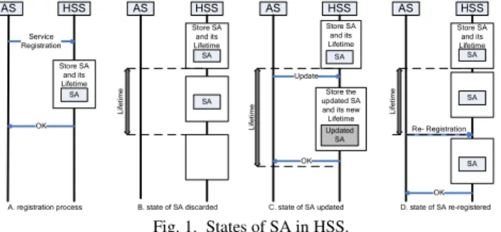
We consider the storage states of service information in LHSS. The service information consists of the SA and its lifetime. When a new service appears, the relevant AS sends its service information by a Service Registration message to the LHSS in the same HSSD, and periodically updates its service information to let LHSS know the service variation in time. When a SA is stored in LHSS, it will be in one of the four states: 1) keeping alive in its lifetime, 2) being discarded when its lifetime is expired, 3) being updated in its lifetime due to the service change, or 4) being re-registered by sending a Re-Registration message before its lifetime is expired. So, a SA keeps valid by being updated or Re-Registered in its lifetime. These conditions are depicted in Fig. 1.
AS HSS Service Registration Store SA and its Lifetime OK A. registration process AS HSS Store SA and its Lifetime L if e ti m e B. state of SA discarded AS HSS Store SA and its Lifetime L if e ti m e Update OK Store the updated SA and its new Lifetime C. state of SA updated SA Updated SA AS HSS OK D. state of SA re-registered SA SA SA Store SA and its Lifetime SA SA L if e ti m e Re- Registration SA Fig. 1. States of SA in HSS.
The proposed novel SDA is illustrated in Fig. 2. The procedure of SD in UE’s own HSSD is described as steps 1-2-3-A-B-4-5-6 and that in a neighbor HSSD is depicted as steps 1-2-3-A-a-b-A'-B'-4-5-6 (including the process of getting a new LHSS address from LSLF). The principle of searching service information is as follows. First, UE looks for its desired service in its own HSSD. If there is no suitable service in its HSSD, it is possible that UE goes on with further searches in its neighbor HSSDs. Whether searching in the neighbor HSSDs and the times of searching are decided by UE depending on the relevant customer’s requirements. The searching order and scope of the neighbor HSSDs are determined by LSLF according to the network topology of LHSSs. LHSS HSSD1 SA1 SA2 … SAn HSSD2 HSSD3 SA1 SA2 … SAn Arrows: 1-2-3-A-B-4-5-6: Searching in UE's HSSD 1-2-3-A-a-b-A'-B'-4-5-6: Searching in a neighbor HSSD UE P-CSCF I-CSCF S-CSCF HSS HSS AS AS LHSS SA1 SA2 … SAn HSS HSS AS AS LSLF SLF SLF LHSS HSS HSS AS AS
Fig. 2. The proposed IMS-based SDA.
The details of SD procedure are expatiated as follows. Here, we only study the steps starting from UE, but those from the customer to UE are not included. Also, the details between UE and Proxy-CSCF (P-CSCF) in the IP connectivity access network are not considered. First, UE searches its desired service information in its own HSSD. A SrvRqt is sent by UE then is forwarded to S-CSCF via P-CSCF and Interrogation-CSCF (I-CSCF). According to the address information of LHSS in its caches, S-CSCF finds and contacts the LHSS in the same HSSD. After receiving the SrvRqt, LHSS searches the matching service information in its database and replies with a SrvRply in case of finding the
Page 2 of 12 IEEE/ACM Transactions on Networking
1 2 3 4 5 6 7 8 9 10 11 12 13 14 15 16 17 18 19 20 21 22 23 24 25 26 27 28 29 30 31 32 33 34 35 36 37 38 39 40 41 42 43 44 45 46 47 48 49 50 51 52 53 54 55 56 57 58 59 60
For Peer Review
suitable service information. Then, the service information is sent back from LHSS to UE in the SrvRply message. After receiving the SrvRply, if there is more than one service fitting the SrvRqt, UE will select the best one. We set an expiration time to each SrvRqt. If there is no SrvRply back to UE during this time interval, UE will reckon that there is no matching service in its HSSD. In this condition, UE may start one or several new searches in its neighbor HSSDs.
The steps of searching in a neighbor HSSD are described as follows. UE sends the same SrvRqt to LSLF through P-CSCF, I-CSCF, and S-CSCF, but set a new expiration time. After receiving the SrvRqt, LSLF chooses the nearest neighbor HSSD based on the network topology and responds to S-CSCF with the corresponding LHSS address information. Then, S-CSCF contacts the new LHSS. After searching in the new LHSS, a new SrvRply is replied to UE (having suitable service) or no response (having no matching service). If there is no matching service in the nearest neighbor HSSD, i.e., UE can not find suitable service the second time, UE may ask LSLF again in the same manner as in its nearest neighbor HSSD to search service in another neighbor HSSD. The process may repeat several times. The times of search and the expiration time of each search are determined by UE according to relevant service requirements including the service priority, the real-time demand, and so on.
Obviously, our SDA is solely based on IMS and only uses the existing entities and functionalities in the IM CN Subsystem. The advantage is that our SDA is well integrated with IMS and can realize the USD function among different access networks based on IMS without adding any new entities or functionalities.
III. MATHEMATICAL MODELING AND THEORETICAL
ANALYSES
In this section, we analyze the performance of our SDA through mathematical modeling and theoretical analyses. We model LHSS as an M/G/c/c queuing system, and evaluate the performance in terms of cache size in LHSS for SAs, success rate of SD, and the relevant traffic load caused by SD procedure. The impacts of the average update interval of SA, the mean interval between two adjacent SrvRqts, and the variation of network conditions are all considered.
A. Cache Size in LHSS for SAs
As described in Section II, in each HSSD, SAs coming from ASs are stored in the database of LHSS and discarded when there is no update or re-registration within their lifetimes. That is, each LHSS stores and deletes SAs according to their lifetimes.
First, we study the state in one HSSD and analyze the cache size for SAs in one LHSS. We assume the arrival of SAs is a Poisson process, the service time of each SA is its lifetime (an SA updated or re-registered is considered as a new SA), and the cache capacity of LHSS for SAs equals to the number of
available services in the HSSD. Then, we model LHSS as an M/G/c/c queuing system [10]. The model is depicted in Fig. 3.
Fig. 3. State transition diagram of LHSS caches.
The parameters in Fig. 3 are defined as follows.
n: the cache capacity of LHSS for SAs. Ek: the state of k SAs stored in LHSS.
λi: the arrival rate of SAs when in the state of Ei. Here, we
assume the average arrival rate of SAs is λ, and set λi=λ, i=0, 1,
…, n-1.
µi: the service rate of SAs when in the state of Ei. We set
µi=iµ, i=1, 2, …, n. µ is defined as the mean service rate of SAs,
and it equals to the mean discarded rate of SAs, i.e., µ=1/TL.
Here, TL is the average lifetime of SAs.
Let HAS-HSS be the mean hop distance between AS and LHSS,
and Pf be the average one-hop loss rate in the network. Then,
the success rate of an SA transmitted from AS to LHSS is derived as
(
1)
HAS HSSAS HSS f
P − = −P − . (1)
Let NAS be the total number of ASs providing services and
assume each AS can only provide one service and send one SA message simultaneously. ISA is denoted as the average update
interval of SA including its registration, update, and re-registration. Then, we have,
AS AS HSS SA
N P I
λ= − (2)
We denote the traffic intensity as ρ=λ/µ. According to the queuing theory [19], the probability of k SAs being stored in LHSS is derived as, 2! 0,1,..., 1 ... 2! ! k k n k P for k n n ρ ρ ρ ρ = = + + + + (3)
Let the average size in bytes of an SA be bSA, and set the
cache capacity of LHSS for SAs n as the total number of ASs
providing services NAS in the same HSSD. Then, the cache size
in LHSS for SAs is computed as
1 2 3 4 5 6 7 8 9 10 11 12 13 14 15 16 17 18 19 20 21 22 23 24 25 26 27 28 29 30 31 32 33 34 35 36 37 38 39 40 41 42 43 44 45 46 47 48 49 50 51 52 53 54 55 56 57 58 59 60
For Peer Review
4(
)
(
)
0 0 0 1 1 ! ! AS HSS AS AS HSS AS n HSS SA SA k k k H AS f L N SA SA j k AS H f L N SA j C b kP N P T I b k N P T I k j − − − = = = = − = − ∑
∑
∑
(4) As mentioned above, we only studied the cache size for SAs in one LHSS covering one HSSD, and the condition in each HSSD is equal in terms of modeling. So, it is not necessary to analyze the cache usage in each LHSS.B.Success Rate of SD
First of all, the success rate of SD in UE’s own HSSD is considered. Under this precondition, all the following requirements should be satisfied: 1) LHSS receives SrvRqt sent by UE, 2) LHSS finds the suitable service information in its database, and 3) UE gets SrvRply responded by LHSS.
We consider the process of sending SrvRqt from UE to
LHSS. Let HUE-HSS denote the mean hop distance from UE to
LHSS. Then, the success rate in this part is
(
1)
HUE HSSSrvRqt f
P = −P − . (5)
We assume the success rate of receiving SrvRply from LHSS to UE is equal to PSrvRqt, namely, PSrvRply=PSrvRqt. The success rate of searching suitable service information in LHSS means the probability of suitable SAs cached in LHSS successfully. We denote the mean interval between two adjacent SrvRqts as ISrvRqt and set
SrvRqt SA I m I = . (6)
Then, ISrvRqt=mISA+x. Here, m=0, 1, 2, …; x=mod(ISrvRqt, ISA), and x [0, ISA).
When its lifetime expires, an SA will be discarded. That means only the latest several transmissions (named valid transmissions) of an SA influence the success rate of storing SA in LHSS. We set ' L SA T m I =
, then have TL=m'ISA+x'. Here, m'=0, 1,
2, …; x'=mod(TL, ISA), and x' [0, ISA).
When x≤x', the number of valid transmissions of an SA is
n1=m'+1, otherwise, it is n2=m'. The possibilities in the two
conditions are P(n1)=x'/ISA and P(n2)=1–P(n1). Then, the success rate of finding a suitable SA cached in LHSS is expressed as
(
)
(
)
1 1 2 2 1 1 , ' 1 1 , ' n SA AS HSS SA n SA AS HSS P P if x x P P P if x x − − = − − ≤ = = − − > (7)(
)
( )
(
)
( )
2 mod( , ) ' mod( , ) ' 1 L SA SA L SA SA T I P x x P I T I P x x P n I ≤ = = > = = − 1 n (8)Assume there are s services in this HSSD matching SrvRqt, then the success rate of SD in UE’s own HSSD is expressed as
(
)
(
1 1
s)
SD SrvRqt SrvRply SA
P
=
P
P
− −
P
(9)The average success rate of SD in UE’s own HSSD is
considered as the expected value of PSD, that is,
(
)
( )
(
(
)
)
( )
(
(
)
)
(
)
(
(
)
)
(
)
(
)
(
)
(
(
)
)
1 2 1 2 2 1 2 1 1 1 1 mod , 1 1 1 1 1 1 mod , 1 1 1 1 1 1 UE HSS L AS HSS SA UE HSS s SD SrvRqt SrvRply SA s SrvRqt SrvRply SA H L SA f SA s T H I f H L SA f SA E P P n P P P P n P P P T I P I P T I P I − − − + = − − + − − = − − − − − − + − − − − − −(
(
1)
)
L AS HSS SA s T H I f P − − (10) If it receives SrvRply including the information of more than one suitable service, UE will choose the best one according to its specific requirements. When there is no suitable service in UE’s HSSD, S-CSCF may communicate with LSLF and continues to search in neighbor HSSDs. Here, we only analyze the procedure of search in UE’s own HSSD because in a neighbor HSSD, the procedure is the same ignoring the communications between S-CSCF and LSLF.C.Traffic Load Generated by SD Procedure
Assume each UE only looks for its desired services in its own HSSD, and in this precondition we analyze the traffic load generated by SD procedure in one HSSD.
Assume there are q SrvRqts and w SAs in a random period of time T. Using the similar analytical method in Subsection B, we derive
Page 4 of 12 IEEE/ACM Transactions on Networking
1 2 3 4 5 6 7 8 9 10 11 12 13 14 15 16 17 18 19 20 21 22 23 24 25 26 27 28 29 30 31 32 33 34 35 36 37 38 39 40 41 42 43 44 45 46 47 48 49 50 51 52 53 54 55 56 57 58 59 60
For Peer Review
( )
(
)
(
)
1 1 2 2 mod , 1, P q mod , , P( ) 1 SrvRqt SrvRqt SrvRqt SrvRqt SrvRqt SrvRqt T I T q I I q T I T q q I I = + = = = = − (11)( )
(
)
( )
(
)
1 1 2 2 mod , 1 , P w mod , , P 1 SA AS SA SA SA AS SA SA T I T w N I I w T I T w N w I I = + = = = = − (12)The number of SrvRplys is determined by the success rates of SrvRqts and SAs, and all the SrvRplys constitute n-time Bernoulli trial. Assume there are r SrvRplys in T, using binomial distribution, we have
(
) (
)
(
)
(
) (
)
0 0 1 ! 1 ! ! q k q k k q SA SrvRqt SA SrvRqt k q k q k SA SrvRqt SA SrvRqt k r kC P P P P q k P P P P k q k − = − = = − = − −∑
∑
(13) The traffic load caused by SAs, SrvRqts, and SrvRplys in T are denoted as LSA, LSrvRqt, and LSrvRply, respectively, then thetotal traffic load in UE’s HSSD can be expressed as
HSSD SA SrvRqt SrvRply
L =L +L +L . (14)
Let mSA, mSrvRqt, and mSrvRply be the number of mean total
messages caused by one SA, SrvRqt, and SrvRply, respectively. We derive
(
)
(
)
1 1 1 AS HSS AS HSS 1 H H i SA AS HSS f f f i m H P iP P − − − − = = − +∑
− (15)(
)
(
)
1 1 1 UE HSS UE HSS 1 H H j SrvRqt UE HSS f f f j m H P jP P − − − − = = − +∑
− (16) SrvRply SrvRqt m =m (17)Using bSrvRqt, bSrvRply, and bSA express the average size of
SrvRqt, SrvRply, and SA in bytes respectively, then we can further derive
SA SA SA
L =wm b (18)
SrvRqt SrvRqt SrvRqt
L =qm b (19)
SrvRply SrvRply SrvRply
L =rm b (20)
We consider the whole IMS-based network including more than one HSSD. Regard the SrvRqts of searching in neighbor HSSDs as new SrvRqts, assume there are H HSSDs in all, and ignore the communications between S-CSCF and LSLF. The total traffic load in the whole IMS-based network can be
calculated approximately as
total HSSD
L =HL (21)
The average traffic load caused by SD procedure in the whole IMS-based network is considered as the expected value of Ltotal, that is,
( ) ( ) ( )
(
)
( ) ( ) ( )
(
)
( ) ( ) ( )
(
)
( ) ( ) ( )
(
)
( ) ( ) ( )
(
)
( ) ( ) ( )
(
)
( ) ( ) ( )
(
)
( ) ( ) ( )
1 1 1 1 1 1 1 2 1 1 2 1 1 1 2 1 1 2 2 1 1 2 1 1 1 2 2 1 2 2 2 2 1 2 2 1 2 1 2 2 1 2 2 2 2 2 2 ( ) , , , , , , , , , , , , , , , , total total total total total total total total total E L P q P w P n L q w n P q P w P n L q w n P q P w P n L q w n P q P w P n L q w n P q P w P n L q w n P q P w P n L q w n P q P w P n L q w n P q P w P n L q w n = + + + + + + +(
2)
(22) We set(
)
( ) ( ) ( )
(
)
(
)
(
)
(
)
(
)
(
)
(
)
(
)
1 1 1 1 1 1 1 1 1 1 1 , , mod , mod , mod ,1 1 1 1 1 UE HSS UE HSS UE HSS total total SrvRqt SA L SA SrvRqt SA SA H H j SrvRqt UE HSS f f f j SrvRqt H j SrvRply UE HSS f f f j E L P q P w P n L q w n T I T I T I H I I I T b H P jP P I b H P jP P − − − − − = − − = = = + − + − + − + −
∑
(
)
(
(
)
)
(
)
(
(
)
)
1 1 1 0 1 1 1 1 1 1 1 1 1 1 UE HSS L SrvRqt UE HSS AS HSS SA SrvRqt L UE HSS AS HSS SA H T k T I H H I k f f T k I T H H I f f kC P P P P − − − − − + + + = + − − − − − − − − − ∑
∑
(
)
(
)
1 1 1 1 1 1 T k ISrvRqt AS HSS AS HSS H H i SA AS AS HSS f f f i SA T b N H P iP P I + − − − − − = + + − + − ∑
(23)(
)
( ) ( ) ( )
(
)
(
)
(
)
(
)
(
)
(
)
(
)
2 1 2 1 1 2 1 1 1 , ,mod , mod , mod ,
1 1 1 1 1 1 UE HSS UE HSS UE HSS total total SrvRqt SA L SA SrvRqt SA SA H H j SrvRqt UE HSS f f f j SrvRqt H SrvRply UE HSS f f E L P q P w P n L q w n T I T I T I H I I I T b H P jP P I b H P jP − − − − − = − = = − + − + − + − + −
∑
(
)
(
)
(
(
)
)
(
)
(
(
)
)
1 1 1 1 1 0 1 1 1 1 1 1 1 1 1 1 UE HSS L SrvRqt UE HSS AS HSS SA SrvRqt L UE HSS AS HSS SA H j f j T k T I H H I k f f T k I T H H I f f P kC P P P P − − − − − − = + + + = + − − − − − − − − −∑
∑
(
)
(
)
1 1 1 1 1 T k ISrvRqt AS HSS AS HSS H H i SA AS AS HSS f f f i SA T b N H P iP P I + − − − − − = + − + − ∑
(24) 1 2 3 4 5 6 7 8 9 10 11 12 13 14 15 16 17 18 19 20 21 22 23 24 25 26 27 28 29 30 31 32 33 34 35 36 37 38 39 40 41 42 43 44 45 46 47 48 49 50 51 52 53 54 55 56 57 58 59 60For Peer Review
6(
)
( ) ( ) ( )
(
)
(
)
(
)
(
)
(
)
(
)
(
)
3 1 1 2 1 1 2 1 1 , ,mod , mod , mod ,
1 1 1 1 1 1 UE HSS UE HSS UE HSS total total SrvRqt SA L SA SrvRqt SA SA H H j SrvRqt UE HSS f f f j SrvRqt H SrvRply UE HSS f f E L P q P w P n L q w n T I T I T I H I I I T b H P jP P I b H P jP − − − − − = − = = − + − + − + − + −
∑
(
)
(
)
(
(
)
)
(
)
(
(
)
)
1 1 1 1 0 1 1 1 1 1 1 1 1 1 UE HSS L SrvRqt UE HSS AS HSS SA SrvRqt T L ISrv UE HSS AS HSS SA H j f j T k T I H H I k f f T k I T H H I f f P kC P P P P − − − − − − = + + = − − − − − − − − − ∑
∑
(
)
(
)
1 1 1 1 1 1 k Rqt AS HSS AS HSS H H i SA AS AS HSS f f f i SA T b N H P iP P I + − − − − − = + + − + − ∑
(25)(
)
( ) ( ) ( )
(
)
(
)
(
)
(
)
(
)
(
)
(
)
(
)
4 2 1 1 2 1 1 1 1 1 1 , , mod , mod , mod , 1 1 1 1 1 UE HSS UE HSS UE HSS total total SrvRqt SA L SA SrvRqt SA SA H H j SrvRqt UE HSS f f f j SrvRqt H j SrvRply UE HSS f f f j E L P q P w P n L q w n T I T I T I H I I I T b H P jP P I b H P jP P − − − − − = − − = = = − − + − + − + −∑
(
)
(
(
)
)
(
)
(
(
)
)
1 0 1 1 1 1 1 1 1 1 1 1 UE HSS L SrvRqt UE HSS AS HSS SA SrvRqt T L ISrvRqt UE HSS AS HSS SA H T k T I H H I k f f T k I T H H I f f kC P P P P − − − − − + = + − − − − − − − − − ∑
∑
(
)
(
)
1 1 1 1 1 k AS HSS AS HSS H H i SA AS AS HSS f f f i SA T b N H P iP P I − − − − − = + + − + − ∑
(26)(
)
( ) ( ) ( )
(
)
(
)
(
)
(
)
(
)
(
)
(
)
5 1 2 2 1 2 2 1 1 , ,mod , mod , mod ,
1 1 1 1 1 1 UE HSS UE HSS UE H total total SrvRqt SA L SA SrvRqt SA SA H H j SrvRqt UE HSS f f f j SrvRqt H SrvRply UE HSS f E L P q P w P n L q w n T I T I T I H I I I T b H P jP P I b H P − − − − − = − = = − − + − + − + −
∑
(
)
(
)
(
(
)
)
(
)
(
(
)
)
1 1 1 1 0 1 1 1 1 1 1 1 1 1 1 UE HSS SS L SrvRqt UE HSS AS HSS SA SrvRqt L UE HSS AS HSS SA H j f f j T k T I H H I k f f T k I T H H I f f jP P kC P P P P − − − − − − = + + = + − − − − − − − − − − ∑
∑
(
)
(
)
1 1 1 1 1 T k ISrvRqt AS HSS AS HSS H H i SA AS AS HSS f f f i SA T b N H P iP P I + − − − − − = + − + − ∑
(27)(
)
( ) ( ) ( )
(
)
(
)
(
)
(
)
(
)
(
)
(
)
6 2 2 1 2 2 1 1 1 , ,mod , mod , mod ,
1 1 1 1 1 1 UE HSS UE HSS UE HSS total total SrvRqt SA L SA SrvRqt SA SA H H j SrvRqt UE HSS f f f j SrvRqt H SrvRply UE HSS f f E L P q P w P n L q w n T I T I T I H I I I T b H P jP P I b H P jP − − − − − = − = = − − − + − + − + −
∑
(
)
(
)
(
(
)
)
(
)
(
(
)
)
1 1 1 0 1 1 1 1 1 1 1 1 1 1 UE HSS L SrvRqt UE HSS AS HSS SA SrvRqt T L ISrv UE HSS AS HSS SA H j f j T k T I H H I k f f T k I T H H I f f P kC P P P P − − − − − − = + = + − − − − − − − − − ∑
∑
(
)
(
)
1 1 1 1 k Rqt AS HSS AS HSS H H i SA AS AS HSS f f f i SA T b N H P iP P I − − − − − = + − + − ∑
(28)(
)
( ) ( ) ( )
(
)
(
)
(
)
(
)
(
)
(
)
(
)
7 2 1 2 2 1 2 1 1 , ,mod , mod , mod ,
1 1 1 1 1 1 UE HSS UE HSS UE HSS total total SrvRqt SA L SA SrvRqt SA SA H H j SrvRqt UE HSS f f f j SrvRqt H SrvRply UE HSS f f E L P q P w P n L q w n T I T I T I H I I I T b H P jP P I b H P jP − − − − − = − = = − − − + − + − + −
∑
(
)
(
)
(
(
)
)
(
)
(
(
)
)
1 1 0 1 1 1 1 1 1 1 1 1 UE HSS L SrvRqt UE HSS AS HSS SA SrvRqt T L k ISrvRqt UE HSS AS HSS SA H j f j T k T I H H I k f f T k I T H H I f f S P kC P P P P b − − − − − − − = = − − − − − − − − − +∑
∑
(
)
(
)
1 1 1 1 AS HSS AS HSS 1 H H i A AS AS HSS f f f i SA T N H P iP P I − − − − = + − + − ∑
(29)(
)
( ) ( ) ( )
(
)
(
)
(
)
(
)
(
)
(
)
(
)
8 2 2 2 2 2 2 1 1 , ,mod , mod , mod ,
1 1 1 1 1 1 UE HSS UE HSS UE H total total SrvRqt SA L SA SrvRqt SA SA H H j SrvRqt UE HSS f f f j SrvRqt H SrvRply UE HSS f E L P q P w P n L q w n T I T I T I H I I I T b H P jP P I b H P − − − − − = − = = − − − − + − + −
∑
(
)
(
)
(
(
)
)
(
)
(
(
)
)
1 1 0 1 1 1 1 1 1 1 1 1 1 UE HSS SS L SrvRqt UE HSS AS HSS SA SrvRqt T L ISrvRqt UE HSS AS HSS SA H j f f j T k T I H H I k f f T k I T H H I f f jP P kC P P P P − − − − − − − = = + − − − − − − − − − − ∑
∑
(
)
(
)
1 1 1 1 k AS HSS AS HSS H H i SA AS AS HSS f f f i SA T b N H P iP P I − − − − = + − + − ∑
(30) Page 6 of 12 IEEE/ACM Transactions on Networking1 2 3 4 5 6 7 8 9 10 11 12 13 14 15 16 17 18 19 20 21 22 23 24 25 26 27 28 29 30 31 32 33 34 35 36 37 38 39 40 41 42 43 44 45 46 47 48 49 50 51 52 53 54 55 56 57 58 59 60
For Peer Review
Then, we have,
(
)
(
)
(
)
(
)
(
15)
(
26)
(
37)
(
48)
( total) total total total total total total total total
E L E L E L E L E L E L E L E L E L
= + + +
+ + + +
(31)
IV. PERFORMANCE ANALYSES AND OPTIMIZATIONS
In this section, we evaluate the performance of the proposed novel SDA by numerical simulations first. All the simulations are based on the analytical models and theoretical analyses deduced in Section III. The input parameters and respective values are documented in Table I.
TABLE I. PARAMETER SETTING.
Parameter Description Value
H The total number of HSSDs in the
whole IMS-based network. 10
NAS The total number of ASs providing
services in each HSSD. 20
T The total simulation time. 1800
seconds
TL The average lifetime of SAs. 150 seconds
HAS-HSS The average hop distance between
AS and LHSS. 2
HUE-HSS The average hop distance between
UE and LHSS. 10
bSA The mean size of SA. 200 bytes
bSrvRqt The mean size of SrvRqt. 50 bytes
bSrvRply The mean size of SrvRply. 100 bytes
ISA
The average update interval of SA. [30, 150] seconds
ISrvRqt The average interval between two
adjacent SrvRqts. [350, 500] seconds
Also, according to the performance analyses, we propose a performance optimization policy based on choosing an optimal value for the average update interval of SA. The policy makes all the performances get the trade-off.
A. Cache Size in LHSS for SAs
Through the analytical expression derived for the cache size in one LHSS for SAs, CHSS-SA in (4), with the average update
interval of SA ISA, the numerical simulation results are
presented in Fig. 4. It is evidently showed that the cache size in one LHSS for SAs, CHSS-SA, decreases while the average update
interval of SA ISA increases. That means reducing the update
frequency of SA can save the cache in LHSS for SAs. On the other hand, the variation of network condition Pf (we set Pf
changes from 0.01 to 0.05) also influences the cache size. But, comparing with ISA, the influence of Pf to CHSS-SA is negligible.
20 40 60 80 100 120 140 160 3,200 3,300 3,400 3,500 3,600 3,700 3,800 3,900 4,000
Average Update Interval of SA (second)
C a c h e S iz e i n O n e L H S S f o r S A s ( b y te ) Pf=0.01 Pf=0.02 Pf=0.03 Pf=0.04 Pf=0.05
Fig. 4. Cache size in LHSS for SAs.
B. Success Rate of SD
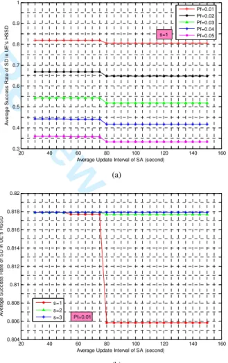
According to the analyses in Subsection B of Section III, the procedure of SD in a neighbor HSSD is the same as that in UE’s own HSSD. So, we only consider the average success rate of SD in UE’s own HSSD here. The simulations are shown in Figs. 5(a) and 5(b).
20 40 60 80 100 120 140 160 0.3 0.4 0.5 0.6 0.7 0.8 0.9 1
Average Update Interval of SA (second)
A v e ra g e S u c c e s s R a te o f S D i n U E 's H S S D Pf=0.01 Pf=0.02 Pf=0.03 Pf=0.04 Pf=0.05 s=1 (a) 20 40 60 80 100 120 140 160 0.804 0.806 0.808 0.81 0.812 0.814 0.816 0.818 0.82
Average Update Interval of SA (second)
A v e ra g e S u c c e s s R a te o f S D i n U E 's H S S D s=1 s=2 s=3 Pf=0.01 (b)
Fig. 5. Success rate of SD.
1 2 3 4 5 6 7 8 9 10 11 12 13 14 15 16 17 18 19 20 21 22 23 24 25 26 27 28 29 30 31 32 33 34 35 36 37 38 39 40 41 42 43 44 45 46 47 48 49 50 51 52 53 54 55 56 57 58 59 60
For Peer Review
8
From the figures, we note that the average success rate of SD
E(PSD) presents the ladder-like decline as the average update
interval of SA ISA is getting longer. The turning point is at the
point of ISA=75 seconds, that is ISA=TL/2 (here, TL is 150
seconds). When ISA is longer than TL/2, the success rate of SD
has a slight reduction. In addition, Fig. 5(a) shows that E(PSD)
descends markedly when the network condition becomes bad, i.e., many signaling messages get lost when Pf increases. In
order to ensure higher success rate of SD, Pf should better not
be higher than 0.02. Also, comparing with the influence of Pf,
the influence of ISA to E(PSD) can be ignored. Take the
condition of S=1 for example. If the average number of matching services for each UE is one, when ISA increases, the
success rate of SD reduces just from 0.818 to 0.806. When the average number of matching services for each UE is more than one (s≥2), the reduction is almost void (see Fig. 5(b), Pf=0.01).
C. Traffic Load Generated by SD Procedure
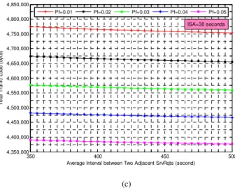
Considering the influence of the average update interval of SA ISA, the mean interval between two adjacent SrvRqts ISrvRqt,
and the network condition Pf, Fig. 6 shows the variation trend
of the average traffic load generated by SD procedure in the whole IMS-based network E(Ltotal).
40 60 80 100 120 140 350 400 450 500 1 2 3 4 5 x 10⁶ Average U pdate Inte rval of SA (second) ISrvRqt (se cond) T o ta l T ra ff ic L o a d ( b y te ) Pf=0.01 (a) 20 40 60 80 100 120 140 160 500,000 1,000,000 1,500,000 2,000,000 2,500,000 3,000,000 3,500,000 4,000,000 4,500,000 5,000,000
Average Update Interval of SA (second)
T o ta l T ra ff ic L o a d ( b y te ) Pf=0.01 Pf=0.02 Pf=0.03 Pf=0.04 Pf=0.05 ISrvRqt=350 seconds (b) 350 400 450 500 4,350,000 4,400,000 4,450,000 4,500,000 4,550,000 4,600,000 4,650,000 4,700,000 4,750,000 4,800,000 4,850,000
Average Interval between Two Adjacent SrvRqts (second)
T o ta l T ra ff ic L o a d ( b y te ) Pf=0.01 Pf=0.02 Pf=0.03 Pf=0.04 Pf=0.05 ISA=30 seconds (c)
Fig. 6. Traffic load generated by SD procedure.
It is observed that the traffic load generated by SD procedure increases when the update frequency of SA improves or/and the SrvRqts come thick and fast, but the traffic load decreases when the network condition is worse. That means prolonging the update interval of SA or/and the interval between SrvRqts, or/and worse network condition can reduce the traffic load. Fig. 6(a) (Pf=0.01) shows that the traffic load decreases sharply
when ISA is getting longer, but ISrvRqt is ignorable comparing to
ISA. On the other hand, the curves of E(Ltotal) metrics for each
different Pf are very close to one another (see Fig. 6(b)
(ISrvRqt=350 seconds)). That means the variety of the network
condition only has a small impact comparing to ISA. Fig. 6(c)
(ISA=30 seconds) presents that E(Ltotal) cuts down as the ISrvRqt
increases, but the impact is slight comparing to Pf. So, the
importance of the influence factors to the traffic load is
ISA>Pf>ISrvRqt.
D. Performance Optimization Policy
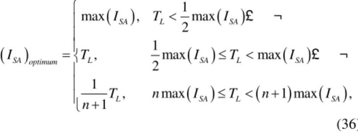
From the above performance analyses, we draw the following conclusions. 1) Prolonging the update interval of SA
ISA saves cache size in LHSS for SAs evidently. 2) There is a
turning point at ISA=TL/2 (here, 30 seconds≤ISA≤150 seconds,
TL=150 seconds). When ISA is longer than TL/2, the average
success rate of SD presents ladder-like reduction. We can get higher success rate by setting ISA≤TL/2. 3) Prolonging ISA
makes the average traffic load generated by SD procedure in the whole IMS-based network decrease much. On balance, we can choose an appropriate ISA to get the best trade-off among
the performances, i.e., we can set ISA slightly less than TL/2 to
satisfy the requirements of higher success rate, less cache space, and lower traffic load simultaneously.
All the above conclusions are based on the parameter setting in Table I. To any arbitrary IMS-based network, now we consider how to find a suitable ISA to get the best trade-off
among all the performances we have analyzed. From Figs. 4, 5, and 6(b), we know the cache size in LHSS for SAs CHSS-SA, the
success rate of SD E(PSD), and the traffic load caused by SD
Page 8 of 12 IEEE/ACM Transactions on Networking
1 2 3 4 5 6 7 8 9 10 11 12 13 14 15 16 17 18 19 20 21 22 23 24 25 26 27 28 29 30 31 32 33 34 35 36 37 38 39 40 41 42 43 44 45 46 47 48 49 50 51 52 53 54 55 56 57 58 59 60
For Peer Review
procedure E(Ltotal) decrease when the ISA increases. In order to
get good performance, both CHSS-SA and E(Ltotal) are the lower
the better, but E(PSD) is the higher the better. According to (4),
(10), and (31), CHSS-SA, E(PSD), and E(Ltotal) are related to ISA.
We use nonlinear optimization theory [20] to get the optimal value of ISA for the sake of optimizing the whole IMS-based
network performances.
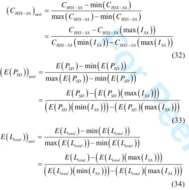
First of all, we use unitary method to deal with (4), (10), and (31), because CHSS-SA, E(PSD), and E(Ltotal) have different
dimensions and units which can not be added directly. After the unitary disposal, we have
(
)
(
)
(
)
(
)
( )
(
)
( )
(
)
(
( )
)
min max min max min max HSS SA HSS SA HSS SA unit HSS SA HSS SA HSS SA HSS SA SA HSS SA SA HSS SA SA C C C C C C C I C I C I − − − − − − − − − − = − − = − (32)( )
(
)
(
(
( )
)
)
(
( )
(
( )
)
)
(
)
(
( )
(
( )
)
)
( )
(
( )
)
(
)
(
( )
(
( )
)
)
min max min max min max SD SD SD unit SD SD SD SD SA SD SA SD SA E P E P E P E P E P E P E P I E P I E P I − = − − = − (33)(
)
(
)
(
(
(
)
)
)
(
(
(
(
)
)
)
)
(
)
(
(
)
(
( )
)
)
(
)
(
( )
)
(
)
(
(
)
(
( )
)
)
min max min max min max total total total unit total total total total SA total SA total SA E L E L E L E L E L E L E L I E L I E L I − = − − = − (34)Then, we try to find the optimal value of ISA to get the best
trade-off among CHSS-SA, E(PSD), and E(Ltotal). Based on the nonlinear optimization theory, we set
( )
(
)
( )
(
)
(
)
(
)
1 2 3 * * * SA HSS SA unit SD unit total unitTrade off I Weight C Weight E P Weight E L − − = − + (35)
Here, Weight1, Weight2, and Weight3 mean the weights of
CHSS-SA, E(PSD), and E(Ltotal), respectively. Considering their
physical meanings, Weight1, Weight2, and Weight3 are all
positive quantities. As mentioned above, both CHSS-SA and
E(Ltotal) are the lower the better, but E(PSD) is the higher the
better. So, in (35), we put the positive signs in front of both
Weight1 and Weight3, but the negative sign in front of Weight2.
As the whole IMS-based network operator, it can set different weights of CHSS-SA, E(PSD), and E(Ltotal) to satisfy the specific
network conditions and requirements. Basically, the setting of weights needs to consider the essential characteristics and special demands of the certain given IMS-based network. For example, if an IMS-based network has limited bandwidths, and
saving bandwidth is the most important aspect comparing with reducing the cost of adding caches in LHSSs for SAs and improving the success rate of SD, the relevant network operator can realize the trade-off among the performances based on the network requirements by adding the weight of
E(Ltotal). Of course, according to different IMS-based networks
or the variations of the same network condition, the network operator can adjust the weights easily and freely. From (35), it is evident that using the expression of Trade-off(ISA), we can
find the optimal value of ISA to get the best trade-off among the
performances according to the requirements of a certain given IMS-based network. Draw the curves of Trade-off(ISA) and
find the corresponding value of ISA which makes Trade-off(ISA)
minimum, and is the optimal value we need.
To be a certain IMS-based network, there are some parameters relatively determinate, such as bSrvRqt, bSrvRply, bSA,
HAS-HSS, HUE-HSS, NAS, and H. For the values of these parameters,
we still use the setting presented in Table I. Also, we still set the total simulation time T to be 1800 seconds. In the following, we discuss the performance optimization policy concretely for choosing the optimal value of ISA.
1) The Influence of the Average Number of Services Matching Each SrvRqt in One HSSD
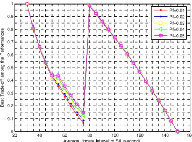
Setting ISrvRqt=350 seconds, Pf=0.01,
Weight1=Weight2=Weight3=1, TL=150 seconds, and the range
of ISA is from 30 to 150 seconds, when the average number of
services matching each SrvRqt s changes from 1 to 3, the curves of Trade-off(ISA) are presented in Fig. 7. It is evident
that the values of s do not influence the selection for the optimal value of ISA. Also, at the point of ISA=TL/2=75 seconds,
we can get the best trade-off among the performances. Here,
TL=max(ISA). 20 40 60 80 100 120 140 160 0 0.1 0.2 0.3 0.4 0.5 0.6 0.7 0.8 0.9 1
Average Update Interval of SA (second)
B e s t T ra d e -o ff a m o n g t h e P e rf o rm a n c e s s=1 s=2 s=3
Fig. 7. Best trade-off for different values of s.
2) The Influence of the Mean Interval between Two Adjacent SrvRqts
We set the average number of matching services for each UE
s=1, Pf=0.01, Weight1=Weight2=Weight3=1 and TL=150
seconds. The value of ISrvRqt changes from 350 to 500 seconds
and ISA ranges from 30 to 150 seconds. From Fig. 8, we see the
value of ISrvRqt does not impact the choice for the optimal value
1 2 3 4 5 6 7 8 9 10 11 12 13 14 15 16 17 18 19 20 21 22 23 24 25 26 27 28 29 30 31 32 33 34 35 36 37 38 39 40 41 42 43 44 45 46 47 48 49 50 51 52 53 54 55 56 57 58 59 60