High speed tracking control of ball screw drives

PAPER • OPEN ACCESS

High speed tracking control of ball screw drives

To cite this article: Chao-Yi Liu et al 2017 IOP Conf. Ser.: Mater. Sci. Eng. 241 012030

View the article online for updates and enhancements.

Related content

Experimental evaluation of a control system for active mass dampers consisting of a position controller and neural oscillator

T. Sasaki, D. Iba, J. Hongu et al.

-Contouring control of ball screw mechanism using a practical control method

Norhaslinda Hasim, Shin Horng Chong, Wai Keat Hee et al.

-Keeping all of the balls in the air Keith S Taber

High speed tracking control of ball screw drives

Chao-Yi Liu1,a_{, Ruei-Yu Huang}b _{and An-Chen Lee}c

1

National Chiao Tung University, Department of Mechanical Engineering 30010 Hsinchu, Taiwan

a

[email protected], [email protected], [email protected]

Abstract. This paper presents a new method to achieve the requirement of high speed and high

precision for ball screw drive. First, a PI controller is adopted to increase the equivalent structural damping in the velocity loop. Next, the design of the position controller is implemented by a two-stage method. The Doubly Coprime Factorization Disturbance Observer (DCFDOB) is developed to suppress disturbance and resist modelling error in the inner loop, while the outer loop is then designed based on method to extend the system bandwidth over first resonant frequency so that high speed and high accuracy can be achieved. Finally, a feedforward controller is implemented to improve tracking performance. The experiment results showed that the proposed method has smaller tracking error and better performance for suppressing disturbance when compared to the conventional cascaded P-PI control.

1. Introduction

Owing to the multiple transmission, the structure of the ball screw system is elastic, which makes actual movement has few differences from input command. These errors will also be magnified during fast motion. Moreover, the machine positioning accuracy will be affected by an external force when machining the workpiece. Therefore, how to fulfill the demand of high speed and high precision is very important in motion control technology.

A. Matsubara et al. [1] and M.S. Kim et al. [2] discussed a common ball screw system model by considering different coupling stiffness effects. S. Frey et al. [3] proposed a discrete model to derive the relationship of the table position and the first resonant frequency. External disturbance and measuring noise are important factors in the motion control. G. L. Luo et al. [4] used acceleration feedback in optimal control to compensate the effect of nonlinear term. K. Ohnishi et al. [5] proposed disturbance observer to suppress the effect from disturbance, noise and uncertainty to system. M. Zatarain et al. [6] predicted positon, velocity and acceleration based on state space observers and used these signals in feedback loop. As to other approaches, the interested reader may refer to [7-9]. The above-mentioned methods, however, have drawbacks to some degree. First, the designed disturbance observer is not optimum in sense of maximum bandwidth under modelling error in [5]. Second, some of them only work well in low frequency range in [7]. Thirdly, most of them did not consider the system change under different table positions except [9] and the others need additional sensor to set up controller [4]. To solve the above problems, this paper presents a new method to achieve the requirement of high speed and high precision for ball screw drive operating higher than the first resonant frequency.

2

The ball screw drive is actuated by applying voltage to a servomotor, which generates a torque to the screw connected to the servomotor by a coupling. Figure 1 shows the dynamic model of the ball screw system. From figure 1, we can obtain the transfer function from torque to table displacement:

3 2 2 2 1 ( ) ( ) ( ) t t t t t t t x RK T  JM s  M DJC s  JKC DR KM s R KC KD s (1)

where T is the input driving torque, xt is the table displacement, Mt is the table mass,

J

is the

rotary inertia, K is the equivalent longitude stiffness, Ct is the damping coefficient of the guideways,

D is the damping coefficient of the rotary motion, Ft is the force to the table, and R is the transform

ratio from shaft angle to table position.

Figure 1. A dynamic model of ball screw system.

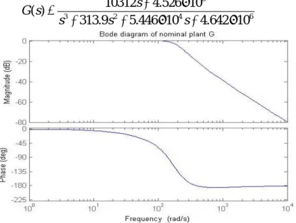
The equivalent stiffness K changes when table moves. This parameter is the major factor on machine vibration. However, as the second resonant frequency is much higher than the first one, we only discuss and design controller for the first resonant frequency. To design the controller easier, we add a PI controller to increase equivalent damping term. The parameters P and I are set 50 and 12, respectively, in underlying experiment. Because the system characteristics change with position, we divide the range of the ball screw into four regions and identify the model independently by using MATLAB system identification toolbox. The nominal plant is chosen by the minimum of the maximum of the gap metric between all models. The obtained nominal plant G s( ) is in equation (2) with its bode diagram shown in figure 2.

6 3 2 4 6 10312 4.526 10 ( ) 313.9 5.446 10 4.642 10 s G s s s s         (2)

3. Controller Design 3.1 DCFDOB Structure

Figure 3 shows the structure of DCFDOB, where the command reference u, the input disturbance di,

the output disturbance do, the estimated input disturbance

d

, the system outputs y, the noise n,

internal states er, ed, en. The actual plant P s( ) is described as right coprime factorization as follow:

1

( n N) ( n M) , ( n, n, N, M )

P N    M    N M   RH (3)

Other factors of corresponding coprime factorization satisfy Eq. 4 as well.

M Y M Y X Y X Y n l n l r r r r I N M N X N X N M n n n l n l n n                                    (4)

where M_n( ),s N s_n( )RH_ are left coprime factorizations of nominal plant ( P_n M N_n1 _n ), and X s Y s X s Y s_r( ), _r( ), _l( ), ( )_l RH_. The notation RH_ is the space of all real rational transfer function matrices without right-half-plane poles. From Fig. 3, the output y is expressed as:

1 2 ( ( )) ( ) ( ) ( ) n n n r i n n t o n n t yP r P IQ IM X  d z  I P QM Y  d z P QM Y 



1 1 1 2

(

)

(

)

(

)

(

)

n n n l n i n n l n o n n r

P r

N



I

N QY N

d

z

M



I

N QY M

d

z

P QM Y



  



















(5)

For suppressing disturbance, we design the controller

Q s

( )



N

_n1

 

J Y

_l1 (where J is a low-pass filter) to make Nn1(I N Q Y Nn D l) n 0

 _{ }

and

M

_n1

(

I



N Q Y M

_{n D l}

)

_n



0

in an acceptable low-frequency range. Then, equation (5) can be rewritten as

n n n r

y

  

P r

P QM Y





. (6)

Thus, the DCFDOB makes the perturbed plant behave like a nominal plant in the low-frequency range and the outer loop controller C s( ) can be designed easily.

Figure 3. Block diagram of DCFDOB. 3.2 Cascade H_ Design Method

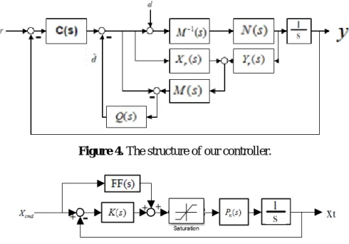
Figure 4 illustrates the control structure, including the inner-loop structure of DCFDOB and the outer-loop position controller. A design procedure which uses cascaded H_ design method is proposed [10]. The inner-loop and outer-loop controllers are then designed as

3 4 2 7 9 4 3 5 2 7 9 50.9 8.568 10 2.509 10 2.041 10 ( ) 797 2.541 10 3.708 10 2.041 10 s s s Q s s s s s               (7) 9 4 12 3 15 2 17 19 5 3 4 7 3 11 2 14 16 2.07 10 5.59 10 1.66 10 2.80 10 2.29 10 ( ) 1.45 10 7.65 10 2.16 10 3.02 10 9.69 10 s s s s C s s s s s s                     (8)

4

Figure 4. The structure of our controller.

Figure 5. The structure of feedforward controller. 3.3 Velocity Feedforward Controller

Feedforward controller is used to improve tracking performance. The structure is shown as Figure 5. The idea of feedforward controller is to make input command and output response perfectly match. So, we design a feedforward controller FF(s) to satisfy equation (9) in low-frequency range. The obtained FF(s)is given in equation (10).

( ( ) ( )) ( ) 1 ( ) ( ) t n cmd n x C s FF s P s x s K s P s      (9) 2 ( 246.7) 1000 (s) (s) 240.5 1000 n s s s FF P s      _{ }    (10) 4. Experimental Results

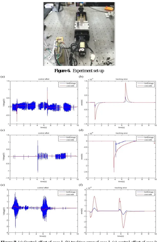
A cascaded controller consisting of position P controller and velocity PI controller called cascaded P-PI is designed as benchmarking. The experiment set-up is shown in figure 6 and the parameters of two controllers are shown in table 1. Three experiments are conducted with results shown in figure 7(a-f). Case 1 used zero input command but added an artificial disturbance signal in the control effort through D/A converter and case 2 added an actual disturbance by applying 350g mass hitting on the moving table. Case 3 performed point-to-point positioning using an S-curve input command determined by the displacement

S



0.2m

, maximum velocity V_max 0.4m/s, maximum acceleration

A

_max



1m/s

2, and average acceleration A_avg 0.6m/s2.

Table 1. The parameters of two controllers.

Parameters

Bandwidth (rad/s)

K_vi Kvp Kpp

Velocity-loop

Position-loop

Cascaded

H_

180

500

12

60

N/A

Figure 6. Experiment set-up

Figure 7. (a) Control effort of case 1, (b) tracking error of case 1, (c) control effort of case 2,

6

Table 2. Result of each experiment

Case Method Control effort (V) Position MSE (m2) Maximum tracking error (m) 1 _{Cascaded H} 3 6.2649 10  9 2.3843 10  4 4.120 10  Cascaded P-PI 3 4.0550 10  8 5.2464 10  3 1.386 10  2 _{Cascaded H} 3 2.1790 10  13 5.2837 10  5 1.302 10  Cascaded P-PI 3 1.9790 10  12 9.3056 10  5 2.531 10  3 _{Cascaded H} 3 9.7926 10  10 2.5422 10  5 6.675 10  Cascaded P-PI 3 6.2259 10  9 6.4876 10  4 3.147 10 

The position mean square error (MSE) and the maximum tracking error of the proposed method are smaller than those of the cascaded P-PI method. The position MSE is about 95.5% less than that of the cascaded P-PI method in case 1, about 94.3% in case 2 and about 96.1% in case 3. The maximum tracking error is about 70.6% less than that of cascaded P-PI method in case 1, about 48.6% in case 2 and about 78.3% in case 3. But the control effort of the method is larger; however, it is under saturation constraint, i.e., it is about 54.5% larger than that of cascaded P-PI method in case 1, about 10.1% in case 2 and about 57.3% in case 3. From the experiment results, our method demonstrates good performance at disturbance suppression and trajectory tracking. Because of no control effort constraint, our controller contains more high-frequency components which leads to faster response.

5. Conclusion

In this paper, a cascaded H_ design method for high speed tracking control of ball screw drives is presented. The experiment results show that this method has better performance in trajectory tracking and disturbance rejection than the cascaded P-PI design method. Though the control effort of our method is larger, it does not violate the driver constraint



10V

.

Acknowledgments

This work was supported by the Ministry of Science and Technology of Republic of China, under Contract MOST 104-2221-E-009 -027 –MY2.

Reference

[1] Matsubara, Y. Kakino and Y. Watanabe 2000 Proc. of 2000 Japan-USA Flex. Auto. Conf [2] M.S. Kim and S.C. Chung 2006 Mechatronics 16 491

[3] S. Frey, A. Dadalau and A. Verl 2012 Product. Eng. 6 205

[4] G.L. Luo and G.N. Saridis 1985 IEEE J. of Robotics and Automation RA-1 152

[5] K. Ohishi, M. Nakao, K. Ohnishi, and K. Miyachi 1987 IEEE Trans. on Ind. Elec. 34 44

[6] M. Zatarain, I. Ruiz de Argandoña, A. Illarramendi, J.L. Azpeitia and R. Bueno 2005 Annals of

CIRP 54 393

[7] A. Verl and S. Frey 2012 Annals of CIRP 61 351

[8] K. Erkorkmaz and Y. Hosseinkhani 2013 Annals of CIRP 62 387 [9] L. Dong, W.C. Tang and D.F. Bao 2015 ISA Trans. 55 219