應用於無線近身網路的動態取樣相位頻率調整技術

全文

(1)國. 立. 交. 通. 大. 學. 電子工程學系電子研究所碩士論文. 應用於無線近身網路的動態取樣相位頻率調整技術 A Dynamic Phase-Frequency Recovery Method for Wireless Body Area Network 研究生 : 楊美慧指導教授 : 李鎮宜博士. 中華民國九十六年七月.

(2) 應用於無線近身網路的動態取樣相位頻率調整技術 A Dynamic Phase-Frequency Recovery Method for Wireless Body Area Network 研究生：楊美慧. Student：Mei-Hui Yang. 指導教授：李鎮宜教授. Advisor：Prof. Chen-Yi Lee. 國立交通大學電機學院電子工程所碩士班碩士論文 A Thesis Submitted to Institute of Electronics College of Electrical and Computer Engineering National Chiao Tung University in partial Fulfillment of the Requirements for the Degree of Master in Electronics Engineering July 2007 Hsinchu, Taiwan, Republic of China. 中華民國九十六年七月 ii.

(3) 應用於無線近身網路的動態取樣相位頻率調整技術研究生: 楊美慧. 指導教授: 李鎮宜國立交通大學電子工程學系電子研究所碩士班. 摘. 要. 近年來無線近身網路的應用已經逐漸受到重視，尤其是應用於人體生醫資訊的偵測，預期可以大大降低醫療成本以及提高醫療成效。在這樣的應用中，偵測點加傳送端會被放在人體上，它的主要訴求會是越低的功率消耗，以避免時常要更換電池的麻煩。接收端可以被整合在手機或是個人數位助理等裝置，主要訴求是提升整個系統的效能，以確保生醫訊號無線傳輸的可靠度。. 本篇論文將介紹一個應用於無線近身網路，結合正交多工分頻及分碼多重存取技術的基頻收發器。正交多工分頻技術具有長的信號週期有利於消除多路徑通道中的選擇性衰減，能符合高速及高傳輸品質要求。分碼多工存取技術提供無線近身網路能同時有多個傳送端傳送資料，同時也提升訊號對雜訊的免疫力。除此之外，本篇論文也將提出應用於此系統的動態取樣相位頻率調整技術搭配一個可以調整相位及頻率的時脈產生器，來避免接收端使用2倍取樣以上的類比轉數位電路，以降低接收端類比轉數位電路的功率消耗達46.45%，而同時，動態取樣相位頻率調整也能針對傳送端和接收端的時脈不協調作偵測及調整，其結果跟傳統的只單純補償資料比較，在AWGN通道的模擬環境上，在傳輸的封包錯誤率達到1 % 時，會使整體的效能提高0.8dB。. i.

(4) A Dynamic Phase-Frequency Recovery Method for Wireless Body Area Network Student: Mei-Hui Yang Advisor: Chen-Yi Lee Department of Electronics Engineering and Institute of Electronics, National Chiao-Tung University. Abstract In this thesis we propose a MT-CDMA baseband processor for Wireless Body Area Network application comprising the dynamic phase and frequency recovery scheme to assure the overall system power reduction and performance improvement.. In recent years, health monitoring has gradually attracted many attentions. In such applications, a transmitter node will be placed on human body for long time monitoring, while the receiver can be bundled into mobile phones or PDAs. Low power demand for transmitter node and good transmission performance is required in this system.. We propose a MT-CDMA system for this application, using the. advantage of orthogonal frequency division multiplexing (OFDM) and code division multiple access (CDMA). Besides that, a dynamic phase and frequency recovery scheme is proposed for power reduction and performance improvement. By the dynamic phase recovery, signal sampling rate is reduced from Nyquist rate (or higher) to the symbol rate, resulting in reduced ADC circuit power. By the dynamic frequency recovery, data is recovered from less-interfered data. In the MT-CDMA system, the simulations show that the system improves 0.8 dB SNR and reduce 46.45% ADC power with the DFR and DPR techniques, respectively.. ii.

(5) 誌謝在 Si2 實驗室從大三專題到碩士班畢業的 4 年時光是我求學過程中最美好的回憶，非常感謝我的指導教授李鎮宜博士，他創造了非常完善的研究環境，使我們有機會從系統的層面與全方位的角度來思考研究的方向。感謝實驗室的游瑞元學長，在碩士班兩年裡給我的指導，也非常感謝我的家庭一直非常支持我，使我能完成碩士學業，最後感謝口試委員的指導與寶貴的意見。. iii.

(6) CONTENTS. PAGE. CHAPTER 1 ..................................................................................................................1 Introduction....................................................................................................................1 1.1 Ubiquitous personal health inspector (UPHI) system......................................1 CHPTER 2 .....................................................................................................................4 Multi-Tone CDMA System............................................................................................4 2.1 Packet format ...................................................................................................8 2.2 Preamble format...............................................................................................8 2.3 Block diagram................................................................................................10 2.3.1 Transmitter ..........................................................................................10 2.3.2 Receiver ..............................................................................................13 2.4 Channel model ...............................................................................................23 2.4.1 Measured channel model around the human body .............................23 2.4.2 Consider the whole indoor environment.............................................24 2.4.3 Consider the channel model when there is relative motion between transmitter and receiver................................................................................25 2.4.4 Consider when there is interference (other sensor node placed nearby) ......................................................................................................................26 2.5 Frequency allocation......................................................................................27 CHPTER 3 ...................................................................................................................29 Dynamic Phase & Frequency Recovery ......................................................................29 3.1 Sampling clock offset ....................................................................................30 3.2 Timing recovery with interpolation ...............................................................31 3.3 Dynamic phase recovery................................................................................35 3.4 Dynamic frequency recovery.........................................................................37 3.5 The structure of phase-frequency tunable clock generator ............................41 CHPTER 4 ...................................................................................................................44 Simulation Result.........................................................................................................44 4.1 Simulation on AD/DA resolution...................................................................44 4.2 Simulation on PER performance with carrier frequency offset and sampling clock offset...........................................................................................................46 4.3 Simulation on dynamic phase recovery .........................................................48 4.3 Simulation on dynamic frequency recovery ..................................................53 CHPTER 5 ...................................................................................................................57 Conclusion and Future Work .......................................................................................57 5.1 Conclusion .....................................................................................................57 iv.

(7) 5.2 Future Work ...................................................................................................59 Reference .....................................................................................................................60. v.

(8) LIST of FIGURES. PAGE. Fig. 1-1, UPHI application.............................................................................................1 Fig. 1-2, The relation of ADC’s power consumption to its sampling speed. .................3 Fig. 2-1, Orthogonal frequency division multiplexing. .................................................5 Fig 2-2, Code division multiple access. .........................................................................6 Fig.2-3, The packet format.............................................................................................8 Fig.2-4, The preamble format. .....................................................................................10 Fig. 2-5, The block diagram of transmitter. ................................................................. 11 Fig.2-6, QPSK mapping...............................................................................................12 Fig.2-7, The data is scheduled before entering IFFT...................................................12 Fig.2-8, The block diagram of receiver........................................................................13 Fig.2-9, Use autocorrelation to detect packet. .............................................................14 Fig. 2-10, Packet detect error rate in different signal to noise ratio with random CFO<120 kHz..............................................................................................................14 Fig.2-11, CFO estimation accuracy..............................................................................16 Fig. 2-12, Log-arctan method to find angle. ................................................................17 Fig. 2-13, Block diagram of binary search method to find angle. ...............................18 Fig.2-14, De-spreading window...................................................................................18 Fig. 2-15, Flow graph of 32-point FFT. .......................................................................20 Fig. 2-16, Human body path loss model. .....................................................................24 Fig. 2-16, System packet error rate with different number of interferences................27 Fig. 3-1, Power comparison of receiver baseband and 2 times over-sampling rate ADC. ......................................................................................................................................30 Fig.3-2(a), Sampling phase offset ................................................................................31 Fig.3-2(b), Sampling frequency offset.........................................................................31 Fig.3-3, The relation of ADC’s power consumption to its sampling speed. ................32 Fig. 3-4, Block diagram with receiver with interpolations to solve symbol timing error. ......................................................................................................................................33 Fig. 3-5, Power consumption of ADC and PFTCG under 90nm CMOS technology. .34 Fig. 3-6, The relationship of estimated phase rotation slope C1,l and OFDM symbol index l . .........................................................................................................................39 Fig. 3-7, Receiver block diagram with dynamic phase and frequency recovery. ........40 Fig. 3-8, The function of PTCG and FTCG. ................................................................40 Fig. 3-9, The block diagram of PFTCG. ......................................................................41 Fig.3-10, Digital control oscillator...............................................................................42 vi.

(9) Fig. 3-11, The control mechanism of the PFTCG. .......................................................43 Fig.4-1, PER comparison of different DAC word length ............................................45 Fig.4-2, PER comparison of different ADC word length ............................................45 Fig. 4-3, PER with 112 kHz carrier frequency offset. .................................................46 Fig. 4-4, PER with 50ppm sampling clock frequency offset and data calibration method [7]....................................................................................................................47 Fig. 4-5, PER with different sampling clock phase offset. ..........................................49 Fig.4-6, SNR loss with different sampling phase offset. .............................................50 Fig. 4-7, Probability distribution of adjusted phase using maximal absolute square sum search at SNR=5dB. .............................................................................................51 Fig. 4-8, Probability distribution of adjusted phase under SNR=3dB and 10dB.........52 Fig. 4-9, PER with the proposed dynamic phase recovery. .........................................53 Fig. 4-10, Sampling frequency tuning with the dynamic frequency recovery.............54 Fig. 4-11, PER with the proposed dynamic frequency recovery..................................55 Fig. 4-12, PER with the proposed dynamic phase and frequency recovery. ...............56 Fig. 4-13, Power comparison of the proposed method to the conventional design. ....56. vii.

(10) LIST of TABLES. PAGE. Table 2-1, System feature comparisons .........................................................................6 Table 2-2, System format summary. ..............................................................................7 Table 2-3, The timing related parameter. .......................................................................7. viii.

(11) CHAPTER 1 Introduction. 1.1 Ubiquitous personal health inspector (UPHI) system The global aging of population grows, health care of chronic patients is more important in recent years. Patient monitoring increases staff efficiency and decreases costs in the care process. It makes clinicians can access patient’s data from patient’s office or patient’s bedside anytime and file the data in hospital. Wireless ECG is a mainly application of health care. Fig. 1-1 shows the profiled diagram of wireless ECG application.. Fig. 1-1, UPHI application.. 1.

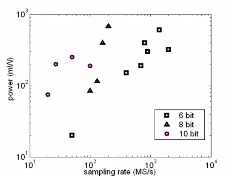
(12) Some systems have been designed for this application domain, e.g. BT, Zigbee, UWB. There can be multiple wireless sensor nodes (WSN) placed on human body, and each sensor nodes perform human data collection, modulation and transmission. The corresponding receiver can be buried into mobile phones as the central processing node (CPN). The UPHI transmitter node design is emphasized on low power, and must be designed in small area, therefore it can be easy to apply and remove, while the receiver is designed to enable a small power-dissipated transmitter and also targeting at low power. Besides that, medical information is sensitive and must to be protected and high transmission quality is also required to ensure the system reliability. Wireless channel effect such as sampling clock offset from transmitter to receiver degrades the system performance largely. Existing wireless system receiver adapts over-sampling for timing recovery of the transmitted data. Over-sampling provides degree of freedom of signal processing for baseband to reconstruct the original data by an interpolation filter. However, over-sampling ADC also causes large power consumption, which is not very suitable in power-limited devices. Fig. 1-2 shows the relationship between ADC sampling rate to its power consumption. The power of ADC is almost directly proportional to its sampling speed. In our developed system, in order to maintain the system performance and reliability and prevent using over-sampling rate ADC for power reduction at the same time, we proposed a dynamic phase recovery method. On the other hand, opposing to the existing sampling frequency offset recovery method: least square estimation of pilot phase error and phase compensation [7], we propose a dynamic frequency recovery method to automatic adjust the sampling frequency and try to eliminate sampling frequency offset to improve system performance under frequency offset distortion. The proposed 2.

(13) dynamic phase-frequency recovery method tries to estimate the sampling clock phase and frequency offset with the aid of a phase-frequency tunable clock generator to drive the ADC sampling in only symbol rate. Thus, with this proposed dynamic phase-frequency recovery, a low power CPN can be attained.. Fig. 1-2, The relation of ADC’s power consumption to its sampling speed.. 3.

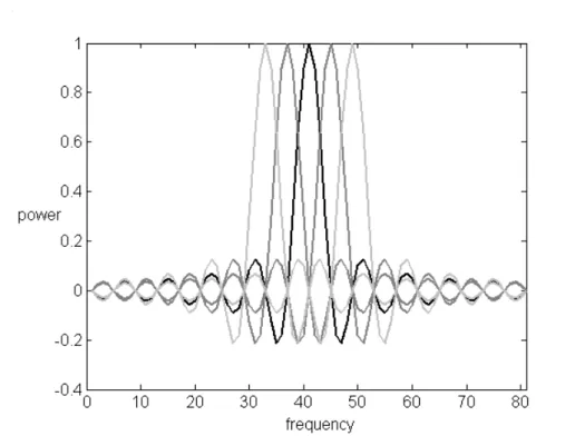
(14) CHPTER 2 Multi-Tone CDMA System. Body signal possesses high correlativity and periodicity. The data rate is only in the order of kbps, which is not very fast. Based on this low data rate property of the UPHI system and to ensure the security and reliability of the overall system, multi-tone CDMA (MT-CDMA) system is applied. It takes both the advantage of OFDM and CDMA techniques. OFDM is an effective modulation technique for high-rate and high-speed transmission over frequency selective fading channels. The available bandwidth is divided into several orthogonal sub-carriers, where the data are shared among, so it can provide better spectral efficiency, as shown in Fig. 2-1. For communications over frequency selective channel, it provides a frequency domain processing technique that contains carrier-by-carrier equalization and mitigates the effects of frequency-selective multipath fading because the fading on each sub-carrier can be taken as being flat.. 4.

(15) In CDMA, the narrowband signal is multiplied by a large bandwidth signal which is pseudo random noise code (PN code), as shown in Fig.2-2. All users in CDMA use the same frequency band and transmit simultaneously. The transmitted signal is recovered by correlating the specified PN code used by the transmitter. Thus, CDMA provides the ability of transmission of multiple users and also the encryption of the transmitted data by the specified PN code.. Fig. 2-1, Orthogonal frequency division multiplexing.. 5.

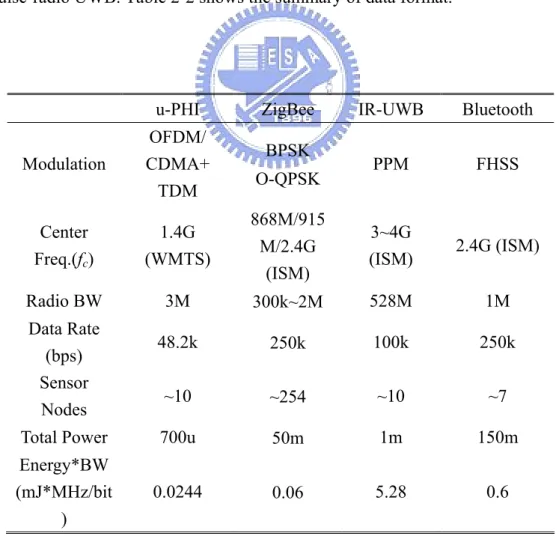
(16) Message. f. Spread spectrum. PN code. f. f. Fig 2-2, Code division multiple access. Table 2-1 lists the system feature comparisons with ZigBee, Bluetooth, and impulse-radio UWB. Table 2-2 shows the summary of data format.. u-PHI. ZigBee. IR-UWB. Bluetooth. PPM. FHSS. 3~4G (ISM). 2.4G (ISM). Modulation. OFDM/ CDMA+ TDM. Center Freq.(fc). 1.4G (WMTS). Radio BW. 3M. 300k~2M. 528M. 1M. 48.2k. 250k. 100k. 250k. ~10. ~254. ~10. ~7. Total Power. 700u. 50m. 1m. 150m. Energy*BW (mJ*MHz/bit ). 0.0244. 0.06. 5.28. 0.6. Data Rate (bps) Sensor Nodes. BPSK O-QPSK 868M/915 M/2.4G (ISM). Table 2-1, System feature comparisons. 6.

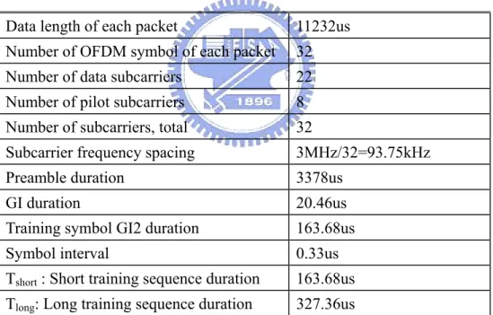
(17) RF Band. 1395~1400MHz. DAC Wordlength. 6. Maximum Data Throughput. 48.2kb/s. User Spreading Code Type. PN Code. Spreading Code Length. 31. Spreading Code Chip Rate. 3Mc/s. IFFT/FFT Block Size. 32. Guard Interval Duration. 20.6 us. Constellation Mapper. QPSK. Coded bits per subcarrier. 2. Data bits per OFDM symbol. 22. Table 2-2, System format summary.. Data length of each packet. 11232us. Number of OFDM symbol of each packet. 32. Number of data subcarriers. 22. Number of pilot subcarriers. 8. Number of subcarriers, total. 32. Subcarrier frequency spacing. 3MHz/32=93.75kHz. Preamble duration. 3378us. GI duration. 20.46us. Training symbol GI2 duration. 163.68us. Symbol interval. 0.33us. Tshort : Short training sequence duration. 163.68us. Tlong: Long training sequence duration. 327.36us. Table 2-3, The timing related parameter.. 7.

(18) 2.1 Packet format. Every packet can be divided into two parts such as the preamble part and the data part, as shown in Fig.2-3. It contains a 3378us long preamble, and totally 32 OFDM symbols that take 11232us to transmit where each OFDM symbol contains 32 symbols and 2-symbols guard interval is inserted between each OFDM symbols.. preamble. 3378us. data 351us × 32 OFDM symbols=11232us. Fig.2-3, The packet format.. 2.2 Preamble format. The preamble consists of three parts. We use the known short preamble without PN code spreading for the purpose of packet detection and carrier frequency offset estimation. It is the shortest part of the preamble, which is only 239.76us long. Next, the short preamble with PN code spreading is transmitted for the purpose of searching of the PN code boundary. The final part is the long preamble which consists of 2 8.

(19) 16-point guard interval and 2 repeated 32-point OFDM symbol, which are for the purpose of channel estimation. The content of short preamble: [0.1021, -0.2939, -0.0299, 0.3167, 0.2041, 0.3167, -0.0299, -0.2939, 0.1021, 0.0052, -0.1742, -0.0281, 0.2041, -0.0281, -0.1742, 0.0052 ]. The content of long preamble 1 (L1) in time domain: [-0.1326, 0.0884, 0.0076, 0.0442, -0.0884, 0.1574, 0, -0.4861, -0.0884, 0.2576, 0, 0.2942, -0.0884, 0.2161, 0, 0.2210, -0.0884, 0.0076, 0, 0.0442, -0.0884, -0.4958, 0, -0.1326, -0.0884, 0.2576, 0, -0.2058, -0.0884, -0.0545, 0]. The content of long preamble 1 (L1) in frequency domain: [-1-j, -1-j, 1+j, -1-j, -1-j, 1+j, 1+j, -1-j, -1+j, -1+j, 1-j, 1-j, -1+j, -1+j, 1-j, -1+j, 1+j, -1-j, 1+j, -1-j, -1- j, 1+j, 1+j, -1-j, -1-j, -1+j, 1-j, 1-j, -1+j, -1+j, 1-j, -1+j ] / 2 . The content of long preamble 2 (L2) in time domain: [-0.1326, 0.0266, -0.0235, -0.0287, -0.0808, 0.1162, 0.2075, -0.3195, -0.3094, 0.1248, -0.1191, 0.2485, 0.1692, 0.0304, 0.1118, 0.0441, 0.2210, -0.1325, 0.1118, -0.1188, 0.1692, -0.3369, -0.1191, -0.2132, -0.3094, 0.2311, 0.2075, -0.2046, -0.0808, -0.0597, -0.0235, -0.1150]. The content of long preamble 2 (L2) in frequency domain: [-1-j, -1-j, 1+j, -1-j, -1-j, 1+j, 1+j, -1-j, -1-j, -1-j, 1+j, 1+j, -1-j, -1-j, 1+j, -1-j, 1+j, -1+j, 1-j, -1+j, -1+j, 1-j, 1-j, -1+j, -1+j, -1+j, 1-j, 1-j, -1+j, -1+j, 1-j, -1+j ] / 2 .. 9.

(20) Synchronization SP SP SP SP SP SP SP SP SP GI. Length. Purpose. L1. L1. GI. L2. L2. Short preamble without spreading. Short preamble with spreading code length 31. Long preamble with spreading code length 31. 333ns*16*45 =239.76us. 333ns*16*9*31=1486.5us. 333ns*(16+32+32)*2*31 =1651.68us. Packet detection & CFO estimation. Search of PN code boundary. Symbol boundary detection & Channel estimation. Fig.2-4, The preamble format.. 2.3 Block diagram. 2.3.1 Transmitter: The WSN side collects data queued in a FIFO or memory. After the FIFO or memory is full, the data will be sent out. The transmitter block diagram is shown in Fig.2-5. We use QPSK mapping the transmitted data in 4 quadrants as shown in Fig.2-6. Before Inverse Fourier transform (IFFT), the mapped data accompanied with pilots are scheduled in order as illustrated in Fig.2-7. The frequency domain spreading is applied in order to make the IFFT-transformed data only contains real parts, that. 10.

(21) means that the imaginary parts are all zeros. By allocating the conjugate of 15th to 1st sub-carriers to 17th to 31st sub-carriers, data after IFFT becomes: 31. X [k ] =. ∑. − j 2π ⋅n⋅k x[n]e 32. n =0 15. =. ∑ x[n] ⋅ (e. j ( (x[ n ]−. n =1 15. =. 2π ⋅n⋅k ) 32. ∑ 2 ⋅ x[n] ⋅ cos((x[n] − n =1. + (e. − j ( (x[ n ]−. 2π ⋅n⋅k ) 32 ). 2π ⋅ n ⋅ k ) 32. ……(2-1). for k = 0 ~ 31. With frequency domain spreading, the transmitter only has to send out one channel of data, thus only one DAC and mixer are needed instead of two, while in the same time the data rate is reduced to half of the original data rate. So we sacrifice data rate to gain the hardware and power reduction in the transmitter side. After the OFDM symbols are formed, all the data are multiplied by a 31 chips PN code known as PN code spreading, and the preamble is added for synchronization demand in the receiver side.. From MAC. QPSK mapping. Pilot insertion. PN code spreading. IFFT. Preamble insertion. Fig. 2-5, The block diagram of transmitter. 11.

(22) Imaginary. 01. 11 1. -1. 1. Real. -1. 00. 10. Fig.2-6, QPSK mapping. data#1 data#2 data#3. pilot. null. pilot data#4 data#5 data#6 pilot data#7 data#8 data#9 pilot data#10 data#11 null data#11* data#10* pilot* data#9* data#8* data#7* pilot* data#6* data#5* data#4* pilot* data#3* data#2* data#1*. pilot*. 0 1 2 3 4 5 6 7 8 9 10 11 12 13 14 15 16 17 18 19 20 21 22 23 24 25 26 27 28 29 30 31. IFFT. Fig.2-7, The data is scheduled before entering IFFT. 12.

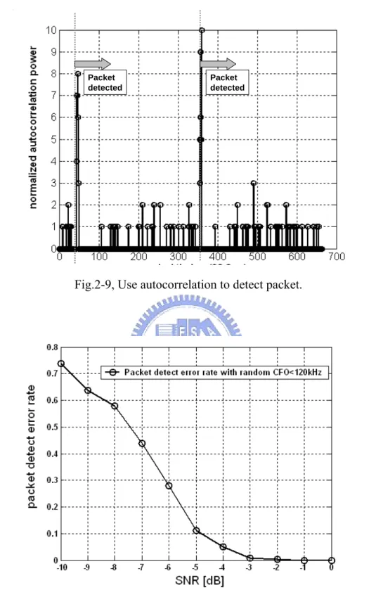
(23) 2.3.2 Receiver. In the receiver side, the block diagram is shown in Fig.2-8. First we use the preamble part to do synchronization including packet detection, CFO estimation, PN code boundary detection and symbol boundary detection.. Packet detection. CFO estimation & compensation. Symbol boundary detection. Phase recovery. FFT. PN code de-spreading. Equalization. QPSK de-mapping. To MAC. Fig.2-8, The block diagram of receiver. Packet detection is done by using 144-point autocorrelation because autocorrelation can detect periodic signal as defined in the initial preamble. The equation is written below where Y[n] is the received data: ∗. Z [n] = Y [n] × Y [n + 144]. 144. Autocorrelation power=. ∑ Z [n ]. 2. ……………………………...(2-2). n =1. And the simulation of auto-correlation result is shown in Fig. 2-9, when the autocorrelation power is larger than a specified level, the packet is claimed to be detected. Fig.2-10 shows the packet detect error rate under signal to noise ratio ranging from -10dB to 0dB plus random carrier frequency offset (<120 kHz), and it shows that packets can be 100% detected even when SNR is 0dB. 13.

(24) Packet detected. Packet detected. Fig.2-9, Use autocorrelation to detect packet.. Fig. 2-10, Packet detect error rate in different signal to noise ratio with random CFO<120 kHz. In a realistic wireless system, the carrier frequency offset from the transmitter to the receiver exists and makes the phase of the received data be rotated, as written in 14.

(25) equation (2-3) where x[n] is the transmitted data, Y[n] is the received data.. Y [n] = X [n] × exp( j × 2 × π × n × CFO / symbol _ rate) ……………………….(2-3) Thus, carrier frequency offset estimation and compensation is needed to recover the transmitted data. We use the periodicity of the preamble to do the CFO estimation. Assume in our developed system, at most 120 kHz carrier frequency offset needs to be solved and the symbol rate is 200ns, and equation (2-3) becomes. Y [n] = X [n] × exp( j × 2 × π × n × 0.024) ……………………………………………(2-4) That means the CFO will make the data phase rotated for 2πin about only 42 symbols which is very serious and the estimation result is also asked to be more accurate. To make the estimation result more accurate, the estimation is divided into two steps. First is the coarse CFO estimation, by using 9 periodic short preambles which only composed of 16 symbols: Y [16 × (k + 1) + n] = Y [16 × k + n] × exp( j 2π × 16 × CFO × (200 × 10−9 )) 16 …………….(2-5) 1 7 1 CFOcoarse = × ∑ ( × tan −1 (∑ (Y [16 × k + n]* × Y [16 × (k + 1) + n]))) 8 k =0 16 n =1. Noted that even with the assumed maximal CFO 120 kHz, the phase rotation between 16 symbols is kept within ±π, so when the estimated result be divided by 16, its correctness will be kept otherwise the positive CFO will be taken as being negative and vice versa. After coarse CFO estimation, the estimation result is used to compensate the received data as written in equation (2-6). z[n] = Y [n] × exp(− j 2π × n × CFOcoarse × 200 × 10−9 ) = Y [n] × (cos(2π × n × CFOcoarse × 200 ×10 −9 ) − j × sin(2π × n × CFOcoarse × 200 × 10 −9 )). ……………………………………………………………………………………..(2-6) The compensated data is further used on fine CFO estimation. Here in order to increase accuracy, we use 9 periodic preambles that spacing 64 symbols to do estimation as written in equation (2-7).. 15.

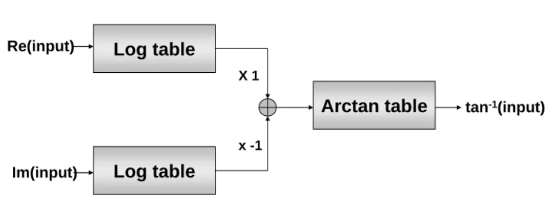
(26) 64 1 7 1 CFO fine = × ∑ ( × tan −1 (∑ (Y [64 × k + n]* × Y [64 × (k + 1) + n]))) ……………. (2-7) 8 k =0 64 n =1. Thus, the total estimated CFO result is CFOcoarse + CFO fine , and we used the result to compensate the incoming data. The simulation of the accuracy of carrier frequency offset estimation is shown in Fig.2-11 with 120 kHz CFO is added. The simulation result shows with both coarse and fine CFO estimation, the resulting root mean square error can be reduced to under 200Hz for SNR larger than 3dB.. Fig.2-11, CFO estimation accuracy.. In the hardware implementation side, the most complex part will be the angle calculation (tan-1), the log-arctan method has been widely used for its special feature that no divider is used [xx]. The input real part and imaginary part are sent into the log table, and log (real part) and log (imaginary part) is obtained. Using log (real. 16.

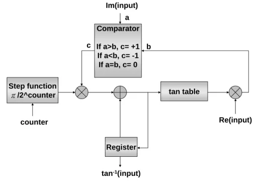
(27) part)-log(imaginary part) to replace real part / imaginary part into the arctan lookup table, as shown in Fig. 2-12.. Re(input). Log table X1. Arctan table. tan-1(input). x -1. Im(input). Log table. Fig. 2-12, Log-arctan method to find angle.. However, in this method, if the input word length is required to be larger than 20 to achieve the CFO estimation accuracy, the log table will become too large as a 2^20 to 1 table. In order to prevent from using divider again, we use a binary search method to derive the desired angle. The block diagram is shown in Fig. 2-13. Its major benefit is that it only contains one lookup table, and the table size only depends on the output word length rather than the input. It uses several steps depending on the accuracy you want to get the nearest angle instead of a one time lookup table. Since the latency of angle calculation is not critical in the CFO estimation, the binary search method is more suitable to reduce the hardware area.. 17.

(28) Im(input) a Comparator c If a>b, c= +1 b If a<b, c= -1 If a=b, c= 0 Step function π/2^counter. tan table. Re(input). counter Register tan-1(input). Fig. 2-13, Block diagram of binary search method to find angle.. After CFO compensation, we use the second part of preamble which contains short preambles with spreading to do PN code boundary detection for de-spreading. While the de-spreading window moves, calculate the cross-correlation power to detect the PN code boundary as shown in Fig. 2-14.. …. … De-spreading window. Fig.2-14, De-spreading window. Cross-correlation power is calculated as in equation (2-8), where Y[n] is the CFO compensated data with de-spreading and X[n] is the known short preamble. As the de-spreading window moves to the correct boundary, cross-correlation will have a peak value. 18.

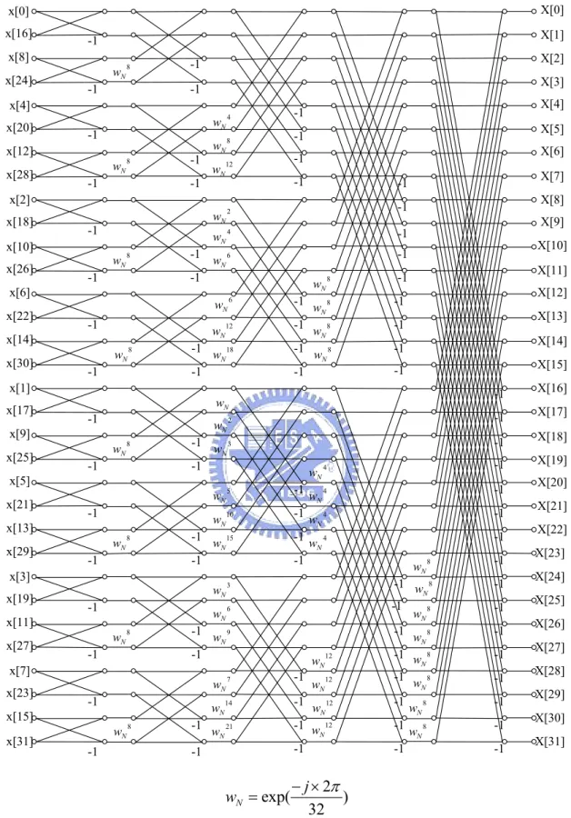
(29) ∗. Z [ n] = Y [ n] × X [ n]. 16. Cross-correlation power=. ∑ Z [ n]. 2. ………………………(2-8). n =1. Long preamble symbol boundary detection is done followed. It uses cross-correlation again. The long preamble and OFDM symbols in the data part are transformed by 32-point FFT into frequency domain. The flow graph of the used 32-point FFT is shown in Fig. 2-15.. 19.

(30) X[0]. x[0] x[16]. X[1]. -1. x[8] x[24]. wN. 8. X[2]. -1. X[3]. -1. -1. x[4] x[20]. -1. x[12] x[28]. wN. 8. -1 -1. -1. wN. 4. -1. wN. 8. -1. 12. -1. wN. X[4] X[5] X[6]. -1. x[2] x[18]. -1. x[10] x[26]. wN. 8. -1. x[6] x[22]. -1. wN. 4. -1. wN. 6. -1. wN. x[14] x[30]. 2. 6. -1. 12. -1. 18. -1. wN. wN. 8. -1. wN. -1. -1. X[8]. -1. wN. -1. -1. X[7]. -1. X[9] X[10] X[11]. -1. wN. 8. wN. 8. -1. wN. 8. -1. wN. 8. -1. X[12] X[13] X[14] X[15]. -1. -1. x[1] x[17]. wN. -1. x[9] x[25]. wN. 8. -1. 2. -1. X[17]. wN. 3. -1. X[18] X[19]. x[5] x[21]. -1. x[13] x[29]. wN. 8. -1. x[3] x[19]. -1. x[11] x[27]. wN. 8. -1. -1. wN. 10. -1. wN. 15. -1. -1 wN. -1. 8. -1. wN. 4. -1. wN. 4. -1. wN. 4. -1. wN. 4. -1. -1 wN. 3. wN. 6. wN. 9. 7. -1. wN. 14. -1. wN. 21. wN. x[15] x[31]. 5. -1. -1. x[7] x[23]. wN. -1. -1. X[16]. wN. -1. -1. -1. wN. wN = exp(. -1. -1. 12. wN. 12. -1. 12. -1. N. wN. -1. wN. 8. -1 -1 -1. wN. 8. -1. wN. 8. -1. -1. − j × 2π ) 32. Fig. 2-15, Flow graph of 32-point FFT.. 20. -1. -1 w 8 N -1 8 wN 8 -1 wN -1 w 8. wN. -1 w 12 N -1. -1. 8. -1. X[20] X[21] X[22] X[23] X[24] X[25] X[26] X[27] X[28] X[29] X[30] X[31].

(31) The long preamble in frequency domain is used for channel estimation as written in equation (2-9).. Y [n] = ( X [n] + w[n]) × H [n] ……………………………………………………...(2-9) H est [n] = Y [n] / X [n]. Since the mapping method in our developed system is QPSK, that means when we do de-mapping, only the angle of the data influences the decoded result. So we only have to equalize the data phase instead of both the phase and magnitude of the data. Thus in the channel estimation side, phase estimation is enough. It can be simplified as in equation (2-10) such that only 2 adders instead of multipliers are needed.. X [n] = (1 + j ) / 2 Y [n] / X [n] = Y [n] × 2 /(1 + j ) ⇒ Y [n] × (1 − j ). ……………………………..(2-10). = Re(Y [n]) + Im(Y [n]) + j × (Im(Y [n]) − Re(Y [ n])). The equalized phase is calculated by log-arctan method as illustrated in Fig.1-11. The equalization step is simplified to phase subtraction and again no multipliers are used. AWGN will cause synchronization error including CFO estimation error. Using pilot phase error tracking, this residual CFO can be compensated by phase recovery. Phase error of frequency signal can be separated as mean phase error caused by residual CFO and linear phase error caused by sampling clock offset. Equation (2-11) shows the influences of residual CFO to the frequency domain signal.. 21.

(32) Time domain signal with residual CFO ∆f in m th OFDM symbol with n th symbol, : x[ m, n] × exp(− j × 2π × ∆f × (m × N + n) × T ). N=34, T=6200ns. Frequency domain signal becomes: 31. X [ k ] = ∑ [x[m,n] × exp(− j × 2π × ∆f × (m × N + n) × T ) × exp(− j × 2π × k × n / 32) ] n=0. 31. = exp(− j × 2π × ∆f × m × N × T )∑ n =0. [ X [ m, n] × exp(− j × 2π × ∆f × n × T ) × exp(− j × 2π × k × n / 64)]. Mean phase error. Inter carrier interference. ……………………………………………………………………………………(2-11). As the residual CFO is < ±1ppm, the inter carrier interference (ICI) error is not obvious, but the mean phase error will increase when OFDM symbol increases. Equation (2-12) shows the influence of sampling clock offset to the frequency domain signal.. FFT{x(t − ∆t )}=X(f) × exp(-j × 2π × f × ∆t) ……………………………………….(2-12). In order to extract these two kinds of phase error, pilot-aided estimation is used. The main idea of that is to solve least square equation (2-13).. T. ⎡1 1 " 1 ⎤ A=⎢ , El = [ El ,1 El ,2 ⋅⋅⋅ El , M ]T , ⎥ ⎣ I1 I 2 " I M ⎦ El , M : phase error on lth OFDM symbol, M th pilot subcarrier ACl = El. ………(2-13). AT ACl = AT El Cl = ( AT A) −1 AT El where Cl = [C0,l. C1,l ]T is the least square solution.. C0,l is the mean phase error, C1,l is the linear phase error slope.. We subtract the estimated phase error in each OFDM symbol, and finally the result is 22.

(33) sent to the de-mapper to decide the output bits.. 2.4 Channel model. 2.4.1 Measured channel model around the human body. Using wireless sensors placed on a person to continuously monitor health information is a new promising application. Therefore the channel model around the human body is recently paid more attention to. Measurements have showed that in the GHz range, the electromagnetic wave will travel around the body rather than pass through the body. In addition, the path loss mechanisms near the body are probably dominated by energy absorption from human tissue which results in an exponential decay of power versus distance. So the path loss near the body is much higher than in free space especially when the transmitter and receiver are placed on the different side of the body. This can be illustrated by that the path loss is usually modeled with the following empirical power decay law:. PdB = P0 dB + 10n log( d / d 0 ) …………………………………………………...(1-14). where n is the path loss exponent, d is the distance from the antenna, d0 is the reference distance(usually set to 0.1m), and the P0dB is the path loss at the reference distance. The measured path loss exponent is n=7.5 around the human body while in the free space, the path loss exponent is n=2. 23.

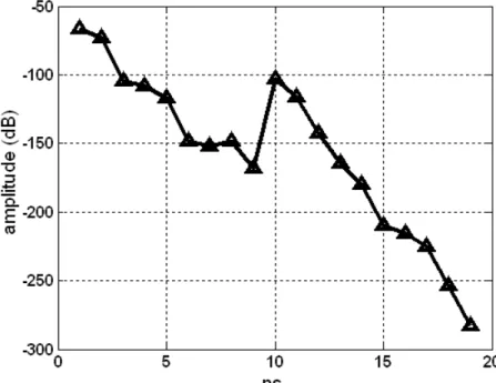
(34) By only considering the human body and ground in the indoor environment, this wireless body area network can be modeled as the measured received power delay profile containing 2 main clusters: one results from the electromagnetic wave diffracting around the body; the other results from the electromagnetic wave reflecting off the ground. To further examining the transmitting amplitude distribution, it has been found that the lognormal model provides a reasonable fit. And because of the symmetry of the human body, the adjacent bins of the measured channel model possess a high correlation property. One of the possible channel models can be plotted as below:. Fig. 2-16, Human body path loss model.. 2.4.2 Consider the whole indoor environment. As the knowledge we know, it is likely that additional multipath component will be. 24.

(35) seen in indoor environment due to reflection of the wall and furniture. The measured channel model result by Saleh and Valenzuela reported a maximum multipath delay spread of 100ns to 200ns within the rooms of a building, and 300ns in hallways. The measured rms delay spread within rooms had a median of 25ns and a maximum of 50ns. The large-scale path loss with no line-of-sight path was found to vary over a 60 dB range and obey a log-distance power law (empirical power decay law) with an exponent n between 3 and 4. Reminded that in our developed system, the guard interval inserted is very long compared to the maximal delay spread as 12.4 us, so almost no ISI will occur. Saleh and Valenzuela developed a simple multipath model for indoor channels based on measurement results. The model assumes that the multipath components arrive in clusters. The amplitudes of the received components are independent Rayleigh random variables with variances that decay exponentially with excess delay within a cluster. The corresponding phase angles are independent uniform random variables over [0 2π]. The clusters and multipath components within a cluster form Poisson arrival process with different rates. The clusters and multipath components within a cluster have exponentially distributed inter arrival times. The formation of the clusters is related to the building structure, while the components within the cluster are formed by multiple reflections from objects in the vicinity of the transmitter and receiver. The corresponding channel model written with Matlab code can be found in the website: http://www.ieee802.org/15/pub/TG4a.html. 2.4.3 Consider the channel model when there is relative motion between transmitter and receiver. Relative motion between the transmitter and receiver causes Doppler shifts in the 25.

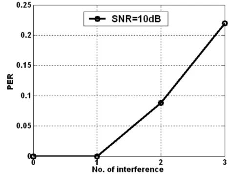
(36) signal frequency. In mobile radio channels, the Rayleigh distribution is commonly used to describe the statistical time varying nature of the received envelope of a flat fading signal, or the envelope of an individual multipath component. The Jakes PSD (power spectral density) determines the spectrum of the Rayleigh process. Since a multipath channel reflects signals at multiple places, a transmitted signal travels to the receiver along several paths that may have different lengths and hence different associated time delays. Fading occurs when signals traveling along different paths interfere with each other [9]-[13].. 2.4.4 Consider when there is interference (other sensor node placed nearby). In realistic application, there can be multiple wireless sensors placed on the human body, each of which is in charge of different monitoring. Besides that, it is also possible that the person near you also wear wireless sensors. Therefore the transmission interference problem needs to be taken into account. One way of differentiate transmitting data of each wireless sensors is by using different PN codes to spread the transmitting signal so that the receiver end can extract the wanted part by dispreading with the corresponding PN codes. Fig.2-16 shows the simulation PER performance with different number of interferences for SNR=10dB.. 26.

(37) Fig. 2-16, System packet error rate with different number of interferences.. 2.5 Frequency allocation. The industrial, scientific and medical (ISM) radio bands were originally reserved internationally for the use of RF electromagnetic fields for industrial, scientific and medical purposes other than communications. These bands are typically given over to uses intended for unlicensed operation, since unlicensed operation typically needs to be tolerant of interference from other devices anyway. For many people, the most commonly encountered ISM device is the home microwave oven operating at 2450 MHz. However, in recent years these bands have also been shared with license-free error-tolerant communications applications such as wireless LANs and cordless phones in the 915 MHz, 2450 MHz, and 5800 MHz bands. In response to growing concerns about interference resulting from the ISM band 27.

(38) devices, the Federal Communications Commission (FCC) established the Wireless Medical Telemetry Services (WMTS), dedicating bands of frequencies for interference-free operation of medical telemetry systems. The WMTS bands are 608 – 614 MHz, 1395 – 1400 MHz, and 1427 – 1432 MHz. All transmitters operating in the WMTS bands must be registered in the database to ensure interference-free operation. Our u-PHI system is designed targeting at 1395 – 1400 MHz WMTS band.. 28.

(39) CHPTER 3 Dynamic Phase & Frequency Recovery. Clock timing recovery is to adjust the sampling timing for each received symbol from analog-to-digital converter and also compensate the signals due to clock phase and frequency offset between the oscillators in transmitter and receiver. In order to solve the symbol timing problem, most OFDM standards set pilot data in an OFDM symbol to do the estimation and compensation of timing error. Pilot symbol aided symbol timing recovery scheme has been investigated and adopted for years. However its effect is still limited for just using the polluted data. In reference [7] [8], a feed-forward timing recovery is proposed with sampling rate that is multiple times of the symbol rate, the timing information can be extracted directly from the received data, the transmitting data then can be easily reconstructed by interpolation among signal samples. With the low-power requirement in about 100mW under 130nm manufacturing process, This implies that the computation complexity of timing phase should be reduced and the ADC operating frequency has to be set as low as possible which usually occupies an equivalent power amount as the one in baseband. Here the power consumption comparison of the MT-CDMA system 29.

(40) receiver baseband and two times over-sampling rate ADC is shown in Fig.3-1. We can see that over-sampling rate ADC consumes about 2/3 baseband power which is we want to reduce. Therefore, to prevent over-sampling rate ADC, we propose a dynamic phase and frequency recovery method with no up-sampled data and still keep about the same performance with sampling clock phase and frequency offset effect.. 2 times over-sampling rate receiver ADC power [14]. 41%. 59%. MT-CDMA receiver baseband power. Fig. 3-1, Power comparison of receiver baseband and 2 times over-sampling rate ADC.. 3.1 Sampling clock offset. With the receiver ADC sampling clock phase and frequency offset, the received data is showed in Fig. 3-2. In Fig. 3-2(a) with the assumption of ADC sampling phase offset ε , the dash line xR represents the sampled data while the opt represents the optimal sampled data. The sampled data all space a fixed time interval to the optimal sampled data. In Fig. 3-2(b) with the assumption that DPR has been done and there is 30.

(41) only sampling frequency offset ζ , the sampled data is represented by the dash lines xR , while again the optimal sampled data is represented by opt . The sampled data space a increasingly time interval to the optimal sampled data. We see that as the symbol index increases, the timing error increases, and this will make the adjusted optimal sampling phase drift away. So we apply DFR to recover the optimal sampling frequency.. x. x. R. x. R. x. ε. ε. R. R. ε. ε. Fig.3-2(a), Sampling phase offset. x. R. x x. R. x. R. R. 2ζ Ts. ζ Ts. 3ζ Ts. Fig.3-2(b), Sampling frequency offset. 3.2 Timing recovery with interpolation. Low power consumption is required especially in wireless personal area network. 31.

(42) (WPAN) [1] and portable devices. In the interpolation approaches, however, received signals are sampled by Nyquist or even higher rate, resulting in large ADC circuit power and dominating the overall system power dissipation. It is shown in Fig. 3-3 that ADC power is about twice as the sampling rate is doubled.. Fig.3-3, The relation of ADC’s power consumption to its sampling speed.. The conventional interpolation method is shown in Fig. 3-4, where the input signal is assumed to be converted to baseband by a free running oscillator. The clock phase Φ estimation is done by using the up-sampled data, followed by the interpolation. coefficients Ck is updated by the estimated clock phase. A data buffer is needed to store I and Q samples to wait for interpolation [3]-[4].. 32.

(43) 2 times upsampling. Received Data. Data Buffer. Interpolation Filter. Output Symbol. Ck Phase Estimator. Φ. Coefficient Update. Fig. 3-4, Block diagram with receiver with interpolations to solve symbol timing error.. Using the interpolation method, not only the sampling timing can be extracted but also the noise interference can be averaged by the interpolation filter. However the major drawback of that is to use 2 times up sampling rate, because it will brings almost 2 times of the ADC power which is not suitable in low power applications.. To meet the system power limitation and reduce the power consumed in an ADC circuit, a dynamic phase recovery (DPR) is proposed to drive the ADC circuits sampling in the symbol rate with the aid of a phase-tunable clock generator (PTCG), which search the best sampling phase in the received signals. To maintain the searched clocking phase without drifting due to clock frequency offset, a dynamic frequency recovery (DFR) accompanied with a frequency-tunable clock generator (FTCG) is also proposed to improve the data recovery performance opposing to the decision-directed phase recovery from noise interfered data.. 33.

(44) The overall system power reduction is made from preventing using over-sampling ADC by adopting a phase and frequency tunable clock generator. The power consumption of these two features is compared in Fig. 3-5. From reference [14] under 90nm process, an ADC with sampling rate 5MHz is about 1.1mW. Doubling the sampling rate will increase its power consumption to around double. However, according to the implementation under 90nm process, the power consumption of a phase-frequency tunable clock generator (PFTCG) is about only 77uW. We can see that they differ by an order amount. So the power reduction is guaranteed.. 3500. power(uW). 3000 2500 2000 1500 1000 500 0 10MHz sampling 1 rate ADC. 5MHz sampling 2 rate ADC. PFTCG 3. Fig. 3-5, Power consumption of ADC and PFTCG under 90nm CMOS technology.. 34.

(45) 3.3 Dynamic phase recovery. ADC clock sampling phase offset will result in worse system performance, thus the dynamic phase recovery (DPR) is applied to recover clock sampling phase. Since we want to keep the ADC sampling rate as the same as symbol rate and also reconstruct the received data with optimal sampling phase, a phase tunable clock generator is required to dynamically adjust the ADC sampling clock phase. The repeated preamble can be used to search the optimal sampling phase. Suppose the transmitter pulse response and receiver analog prefilter are considered as an equivalent response. f (t ) = fT (t ) ∗ f R (t ) …………………………………………………………(3-1) and let fε [n] = f [(n − ε )Ts ], 0 ≤ ε ≤ 0.5 , ε represent the ADC clock sampling phase offset. The optimum sampling phase ε opt is defined that makes a maximum ratio of signal to inter-symbol interference power ratio (SIR), as written in equation (3-2).. ε opt = arg max( ε. fε [0] ∞. ∑. n =−∞. 2. f ε [ n]. 2. ) ……………………………………………………(3-2). n≠0. The normalized received data power can be expressed as E{| xR ,ε |2 } = ∑ fε [n] + σ w ……………………………………………………(3-3) 2. 2. n. where σ w2 is the noise power. Equation (3-3) can be arranged as 35.

(46) E{| xR ,ε |2 } = ( SIR + 1) I + σ w ……………………………………………………….(3-4) 2. where I = ∑ | fε [n] | . Equation shows that with the optimum sampling phase ε opt , a 2. n≠0. 2 maximum E{| xR ,ε | } is obtained. So we may rewrite equation (3-4) as. ε opt = arg max( E{| xR ,ε |2 }) ……………………………………………………….(3-5) ε. Since the expect value E{.} is impossible to get realistically, the power calculation can be done by averaging of finite samples. We use the maximum-absolute-squared-sum (MASS) search of the initial preamble, which is to search for the maximum of the sum of the absolute squared value of the data. Each OFDM symbol of the preamble is sampled using different sampling phases ε , provided by the phase-tunable clock generator. (PTCG),. then. choose. the. phase. that. results. in. the. maximum-absolute-squared-sum to be the sampling phase εˆ . Moreover, the carrier frequency offset caused by the carrier frequency mismatch between transmitter and receiver will not affect the absolute value, because it only makes the received signal phase rotation in time domain, as shown in equation (3-6). ˆxR [ n ] = xR [ n ] ⋅ exp ( j 2π ⋅ f ⋅ n ⋅ TS ) …………………………………….....(3-6). where f is the carrier frequency offset and TS is the symbol period. Therefore the MASS search can be started as soon as the packet detection is done. In order to increase the estimation accuracy, the comparison can be done more than once. For example, we can first choose half of the applying phase with maximal absolute value. 36.

(47) search, and then perform it again on the searched phases in last step and so on.. 3.4 Dynamic frequency recovery. Although dynamic phase recovery adjusts the sampling clock phase, the drift amount due to sampling clock frequency offset still increases. The most significant effect of sampling clock frequency offset is the phase rotation to received subcarriers as written in equation (3-7).. Yl ,k = e. j 2π ( klζ +ε ). TS Tu. X l ,k sinc( π kζ )H l ,k + Nζ ;l .k + Wl ,k …………………......(3-7). where H l ,k is channel frequency response at. k-th subcarrier, Tu is the useful data. portion, Wl ,k is the additive white Gaussian noise and the Nζ ;l ,k is additional noise due to clock sampling frequency error at l-th symbol and k-th subcarrier. Clearly, the phase error is proportional to the symbol index, subcarrier index and sampling clock frequency offset. However, the decision-directed phase recovery method is incapable of recovering the increasing phase error when the drift amount becomes large. Dynamic frequency recovery not only directly compensates the phase error of data after FFT but also tunes the sampling frequency of ADC to eliminate the sampling clock frequency offset. As a result of the small clock frequency offset ζ , the factor sinc(πkζ) in equation (3-7) approximates to one. ADC clock sampling phase offset ε is assumed to be. 37.

(48) zero.. Yl ,k = e. j 2π klζ. TS Tu. Pl ,k H l ,k ……………………………………………………………(3-8). Based on measuring the phase difference between the pilots, the phase error is. El , I m = arg(. Yl , I m Pl , I m H l , I m. ) = 2πI m lζ. TS ………………………………………………...(3-9) Tu. where Pl ,I m is the received data on pilot position at l-th symbol and Im-th subcarrier which is also the pilot index. In order to estimate clock frequency offset, we use the least squares algorithm [7] which can track the residual carrier frequency offset and clock sampling frequency offset.. The clock sampling frequency offset can. accurately estimated as equation (3-10) T. ⎡1 1 " 1 ⎤ A=⎢ , El = [ El ,1 El ,2 ⋅⋅⋅ El , M ]T , ⎥ ⎣ I1 I 2 " I M ⎦ El , M : phase error on l th OFDM symbol, M th pilot subcarrier ACl = El AT ACl = AT El Cl = ( AT A) −1 AT El where Cl = [C0,l. C1,l ]T is the least square solution.. C0,l is the estimated residual CFO, C1,l is the estimated clock frequency offset. …..………………………………………………………………………………(3-10). C1,l is the estimated sampling clock frequency offset in equation (3-9).. C1,l = 2π lζ. Ts …………………………………………………………………...(3-11) Tu 38.

(49) Then, the estimated sampling clock frequency offset at l-th symbol can be easily calculated by equation (3-12).. ζˆl =. Tu × C1,l ………………………………………………………………(3-12) 2π TS × l. Because the additional noise Nζ;l,k due to clock sampling frequency offset and the inter-channel interference (ICI), the result of clock sampling frequency offset estimation is not very stable. And from equation (3-11), we can see that the calculation result C1,l is proportional to the sampling clock frequency offset ζ , and is increasing with the OFDM symbol index l as shown in Fig. 3-6. Thus in order to increase the estimation accuracy and prevent burst errors, we solve the least square equation again to extract the sampling clock frequency offset ζ .. C 1,l. l. Fig. 3-6, The relationship of estimated phase rotation slope C1,l and OFDM symbol index l . 39.

(50) The overall system receiver block diagram with dynamic phase-frequency recovery is shown in Fig. 3-7. After packet detection, the dynamic sampling phase is turned on to adjust the ADC sampling clock to the optimal phase, and the dynamic sampling frequency estimation is also turned on after data processed through the FFT. The Timing error detector performs MASS search while the Frequency error detector performs least squares algorithm. The ADC sampling clock is controlled by PTCG and FTCG, showed in Fig. 3-8.. εˆ Dynamic Dynamicphase phase recovery recovery Packet Packet detection detection. ADC ADC. PFTCG PFTCG. FFT FFT. CFO CFOestimation estimation &&compensation compensation. Equalization Equalization. Symbol Symbolboundary boundary detection detection. PN PNcode code de-spreading de-spreading. Phase Phase recovery recovery. QPSK QPSK de-mapping de-mapping. To MAC. ζˆ. Dynamic Dynamicfrequency frequency recovery recovery. Fig. 3-7, Receiver block diagram with dynamic phase and frequency recovery.. TS TS. Fig. 3-8, The function of PTCG and FTCG.. 40.

(51) 3.5 The structure of phase-frequency tunable clock generator. The PFTCG architecture is shown in Fig. 3-9. The reference clock is generated by the crystal oscillator circuit. The PFD detects the difference of frequency and phase between the reference clock (REF_CLK) generated by crystal oscillator circuit and the DCO (digital clock oscillator) output (FB_CLK). DCO is composed of several delay cells, and they constitute several delay paths, as shown in Fig.3-10. The UP and DOWN signals indicate that the controller adjusts the DCO control code to select the delay path, thus, a frequency-tunable ability is reached. For generating the multiphase clock signal, different phase is extracted in the delay path, too. (By selecting the output position) [6].. Frequency Offset Estimated REF_CLK. UP. PFD. DOWN. Controller. LOCK. Phase _Select FB_CLK. DCO_CODE PHASE 7. DCO. .. .. PHASE 0. Fig. 3-9, The block diagram of PFTCG.. 41. MUX. OUT_CLK.

(52) IN. Buffer. Buffer. Buffer. ……. Buffer. 0. MUX. MUX. ON [ M]. ON [M -1 ]. ……. MUX MUX. ON[1]. ON [0]. OUT. Fig.3-10, Digital control oscillator. The PFTCG control flow is illustrated in Fig. 3-11. After the system reset, the DCO is tuned by the PFD to catch up the speed of the reference clock. The tuning time will last for a fixed period, then the LOCK signal gets high. Afterwards, the DCO is continuously tuned by the estimation of sampling frequency offset which was done by pilot-aided phase recovery.. 42.

(53) System Reset. Update DCO Code. UP. DOWN. PFD. LOCK. Calculate DCO Code. Tune DCO by Phase Recovery. Reset DCO Reset PFD. Calculate & Update DCO Code. Fig. 3-11, The control mechanism of the PFTCG.. 43.

(54) CHPTER 4 Simulation Result. 4.1 Simulation on AD/DA resolution The simulation environment that contains MT-CDMA baseband transceiver and channel model is established by high-level language. Simulation of optimal AD/DA resolution will find a optimal AD/DA word length with the trade-off between error rate performance and hardware complexity. As the word length increases, the computation resolution will also increase and the transmission performance will be better while in the same time more hardware or power consumption is needed. Transmission without any quantization error provides an ideal referenced performance for simulation of the fixed-point transceiver. Fig. 4-1 shows the PER curves of different transmitter DAC resolution. Here we choose DAC word length to be 5 because the performance loss is only 0.5dB at PER=1% which is in the acceptable region. In another way, the simulation of different receiver ADC word length to the overall PER performance is shown in Fig. 4-2. We choose the word. 44.

(55) length to be 6 for the SNR loss is only 0.2 dB at PER= 1% compared to the floating point case.. choice. Fig.4-1, PER comparison of different DAC word length. choice. Fig.4-2, PER comparison of different ADC word length 45.

(56) 4.2 Simulation on PER performance with carrier frequency offset and sampling clock offset. Carrier frequency mismatch between transmitter and receiver leads the received data be distorted, so a compensation scheme is needed to recover the original signal. In our developed system, the CFO estimation is divided into two steps to increase the estimation accuracy: one is coarse CFO estimation and the other is fine CFO estimation. Then use the estimation result to compensate the received data and in Fig.4-3, the simulation of PER with 112 kHz carrier frequency offset is shown. The performance loss is about 0.7dB compared to 0 kHz carrier frequency offset when PER reaches 1%.. Fig. 4-3, PER with 112 kHz carrier frequency offset.. 46.

(57) Sampling clock offset influences the received sampled data, and the offset timing interval will even increase and it may make some data lost. Especially in our developed system, 31-point PN code spreading is performed, so every data symbol is spread to 31 symbols. The timing offset is increasing among the 31 symbols making the de-spread data be largely distorted. Existing frequency offset method is pilot-aided data calibration [7]. It is to estimated data phase rotation caused by sampling frequency offset, and to compensate the data by subtract the estimated phase error. Fig. 4-4 shows the simulated PER with different sampling clock offset with the reference recovery method [7]. In the simulation result, we can see that the performance loss of 50ppm sampling clock offset compared to no frequency offset case is still 1dB at PER=1%, so the reference method is not very robust.. 1dB. Fig. 4-4, PER with 50ppm sampling clock frequency offset and data calibration method [7].. 47.

(58) 4.3 Simulation on dynamic phase recovery. In chapter 3, we have discussed the sampling clock phase offset. Worse sampling phase will lead to large performance degradation. We want to examine on how the sampling phase offset influences the system performance, so by dividing the sampling timing to 8 different phases with equivalent interval noted by. ε = {±0.5, −0.325, −0.25, −0.125, 0, 0.125, 0.25, 0.325} ………………………...(4-1). The simulation was done with the assumption of these phases, and is shown in Fig. 4-5. Because of the symmetry of these sampling phase offsets, we only show 5 phases in Fig. 4-5. It can be inferred that positive offset and negative offset with the same amount will result in the same performance. The simulation result tells that as the phase offset increases, the PER gets worse. The worst case is ε =0.5, and the performance loss is about 2dB at PER=1% compared to no phase offset.. 48.

(59) Fig. 4-5, PER with different sampling clock phase offset.. The proposed dynamic phase recovery is to do maximum absolute value search of the initial preamble with different sampling phases provided by a phase-frequency tunable clock generator. According to the proposed method, optimal sampling phase will provide maximal signal power, so we calculate the maximum absolute value of the sampled data while changing the sampling phase, and choose the phase that result in maximal value to be the estimated optimal sampling phase. Number of phase tunable choices increasing can help the optimal phase search to find the sampling phase that is nearest to the optimal one. However, the sampling phases provided by phase-tunable clock cannot be infinite. In Fig. 4-6, the SNR when PER=1% with. 49.

(60) different amount of sampling phase offset is simulated. Here we choose the acceptable sampling phase offset to be 1/16 which means we need an 8-phase tunable clock generator to do the optimal phase searching.. choice. Fig.4-6, SNR loss with different sampling phase offset.. The simulation result on probability distribution of phase searching is shown in Fig. 4-7 with a 8-phase tunable clock generator and at SNR=5dB. Here we calculate 128-point absolute square sum and the comparisons are performed three times. First we pick up the top four with maximal absolute square sum, then two of the four, then one of the two. Finally the optimal sampled phase can be decided. Noted that the estimation accuracy will be affected by noise as shown in Fig. 4-8, the probability of adjusted phase result under SNR=3dB and 10dB is simulated. We can see that in the SNR=10dB condition, there is about 13.4% more probability lies in the 50.

(61) region that phase offset is zero, while comparing with SNR=3dB condition.. ε Fig. 4-7, Probability distribution of adjusted phase using maximal absolute square sum search at SNR=5dB.. 51.

(62) ε Fig. 4-8, Probability distribution of adjusted phase under SNR=3dB and 10dB. From the simulation results showed above, we can see that most of the probability distribution of phase adjustment lies in the region that makes the better packet error rate. And the overall system performance applying the proposed dynamic phase recovery method is also simulated. It is shown in Fig. 4-9. PER of perfect case (sampling phase offset ε =0) is also drawn in the same plot as a comparison. Originally with the best and worst sampling phase offset, there is about 2.05dB SNR loss. After applying the dynamic phase recovery, through a phase searching and tuning scheme, the resulting SNR when PER equals to 1% can be reduced for 1.9dB.. 52.

(63) Fig. 4-9, PER with the proposed dynamic phase recovery.. 4.3 Simulation on dynamic frequency recovery. In the dynamic frequency recovery method, the sampling frequency offset is estimated by pilot symbol phase rotation in each OFDM symbol. According to equation (3-7), the phase rotation of data in frequency domain is proportional to the OFDM symbol index and data index. With this characteristic, by solving least square equation, we can get the constant and slope terms, and the slope can be referred to the wanted sampling frequency offset. In order to increase estimation accuracy again, the 53.

(64) least square equation is solved two times, one is aiming at a single OFDM symbol, and another is at several OFDM symbols with the estimated result of last step. Fig. 4-10 shows the simulation result of sampling frequency adjustment while using the proposed dynamic frequency recovery. We assume the initial sampling frequency offset be 50ppm. Here the frequency tuning is done once 8 OFDM symbols. In the realistic application, the training packet might have to be sent in advance to get the better sampling frequency. And the overall system performance is also simulated with the proposed dynamic frequency recovery, and is shown in Fig. 4-11. With the proposed dynamic frequency recovery, packet error rate of 50ppm sampling frequency offset case can be kept close to the case of no frequency offset, and there is about 0.2dB SNR loss when PER equals 1%.. convergence. Fig. 4-10, Sampling frequency tuning with the dynamic frequency recovery.. 54.

(65) 0.8dB. Fig. 4-11, PER with the proposed dynamic frequency recovery. In the end, the simulation of both dynamic phase and frequency recovery with 50ppm frequency offset and random phase offset is shown in Fig.4-12. Comparing with the no sampling offset case, there is about only 0.25dB SNR loss when PER=1%. And the overall power comparison designed by 90nm CMOS process is shown in Fig. 4-13. The overhead of the proposed design includes the extra hardware of dynamic phase and frequency recovery and a phase-frequency-tunable clock generator. By replacing the 2 times over-sampling rate receiver ADC circuit with the proposed design, about 46% ADC power can be reduced.. 55.

(66) Fig. 4-12, PER with the proposed dynamic phase and frequency recovery.. 90nm CMOS technology Supply voltage: 1V. 6000 46%. power(uW). 5000 4000 3000 2000. 2X ADC. 1000 0. 1 conventional. 1X ADC. PFTCG(77uW,1.28%) DPR+DFR(140uW,2.33%) ADC[14]. 2 proposed. Fig. 4-13, Power comparison of the proposed method to the conventional design.. 56.

(67) CHPTER 5 Conclusion and Future Work. 5.1 Conclusion. A multi-tone CDMA system is established for wireless body area network application. By using the advantage of orthogonal frequency division multiplexing (OFDM) and code division multiple access (CDMA), the proposed system is very robust to the frequency selective multipath fading and noise interference. Packet error rate can be kept under 1% when SNR>=3dB. The carrier frequency offset up to 112 kHz between transmitter and receiver can also be solved by CFO estimation and compensation proposed in the system.. Besides that, in accordance with sampling clock phase offset between transmitters and receivers, the performance loss from the worst phase to the best one is about 2dB 57.

(68) SNR, so we proposed a dynamic phase recovery method to estimate the phase offset and directly adjust the ADC sampling phase. With the proposed method, the performance loss when there’s phase offset to the perfect case can be kept smaller than 0.15dB SNR.. Sampling clock frequency offset also influences the system performance. The performance loss with 50ppm frequency offset is about 1dB SNR. So a dynamic frequency recovery is also proposed to resist sampling clock frequency offset. It uses pilot sub-carriers of each OFDM symbol to estimate sampling frequency offset and directly adjust the ADC sampling frequency. With the proposed method, there is about 0.8dB SNR improvement under 50ppm frequency offset case.. Considering both the sampling phase and frequency offset, with the proposed dynamic phase and frequency recovery method under 50ppm frequency offset and random phase offset case, there’s only 0.25dB SNR loss to the perfect case. Using dynamic phase recovery can prevent using over-sampling rate ADC in the receiver side. This will induce about 46.38% of ADC power reduction. Using dynamic frequency recovery improves system performance because it deals with the ADC sampling frequency offset not only compensate the received data but also adjusting the ADC sampling frequency to the optimal one.. 58.

(69) 5.2 Future Work. In the future, the following work is to the integration of the digital baseband and the analog RF front-end. Through the integration, the data can be truly transmitted wirelessly, and some potential existing problem such as RF filtering distortion, I/Q mismatch, synchronization problem or the real channel model for indoor and outdoor can be extracted and modeled in the software. Based on this progress, the multi-tone CDMA baseband system can be re-designed and improved to become more robust.. 59.

(70) Reference. [1] IEEE P802.15 Working Group for Wireless Personal Area Networks, “Multi-band OFDM Physical Layer Proposal Merger #1 for IEEE 802.15.3a”, March, 2004. [2] IEEE 802.11 Working Group for Wireless Local Area Networks, http://www.ieee802.org/11/ [3] F. M. Gardner, “Interpolation in Digital Modems – Part I: Fundamentals,” IEEE Trans. Commun., vol. 41, pp. 501-507, Mar. 1993. [4] F. M. Gardner, “Interpolation in Digital Modems – Part II: Implementation and Performance,” IEEE Trans. Commun., vol. COM-41, pp. 998-1008, June 1993. [5] Jui-Yuan Yu, Chin-Che Chung, Hsuan-Yu Liu, Yu-Wei Lin, Wan-Chun Liao, Terng-Yin Hsu and Chen-Yi Lee, “A 31.2 mW UWB baseband Tranceiver with All-Digital I/Q-mismatch Calibration and Dynamic Sampling,” IEEE Symposium VLSI Circuits, pp. 290-291, June, 2006. [6] Chin-Che Chung and Chen-Yi Lee, “A New DLL-based Approach for All Digital Multiphase Clock Generation,” IEEE journal of Solid-State Circuits, vol. 39, pp. 469-475, March 2004. [7] Hung-Kuo Wei, Chen-Yi Lee, “A Frequency Estimation and Compensation Method for High Speed OFDM-based WLAN System,” M.S thesis, Dept. Electron. Eng., NCTU, Taiwan, 2003. [8] Zhu W.-P., Ahmad M.O., Swamy M.N.S., “A fully digital timing recovery scheme using two samples per symbol,” 2001 IEEE Symposium on Circuits and Systems, Vol. 2, PP.421-424, May 2001. [9] Andreas F. Molisch, Kannan Balakrishnan, Chia-Chin Chong, Shahriar Emami, Andrew Fort, Johan Karedal, Juergen Kunisch, Hans Schantz, Ulrich Schuster, Kai Siwiak, ”IEEE 802.15.4a channel model – final report.”. 60.

(71) [10] Fort, A.; Desset, C.; Ryckaert, J.; De Doncker, P.; Van Biesen, L.; Donnay, S.; “Ultra Wide-band Body Area Channel Model,” 2005 IEEE international conference on communication, Vol. 4, PP.2840-2844, May 2005. [11] Zasowski, T.; Meyer, G.; Althaus, F.; Wittneben, A.; ”Propagation Effects in UWB Body Area Networks,” 2005 IEEE international conference on Ultra_Wideband, PP,16-21, Sept. 2005. [12] Kovacs, I.; Pedersen, G.; Eggers, P.; Olesen, K.; “Ultra Wideband Radio Propagation in Body Area Network Scenarios,” 2004 IEEE Eighth Symposium on Spread Spectrum Techniques and Application, PP. 102-106, Aug. 2004. [13] Zasowski, T.; Althaus, F.; Stager, M.; Wittneben, A.; Troster, G.; “UWB FOR NONINVASIVE WIRELESS BODY AREA NETWORKS:CHANNEL MEASUREMENTS AND RESULTS,” 2003 IEEE conference on Ultra-Wideband Systems and Technologies, PP. 285-289, Nov. 2003. [14] Geelen, G.; Paulus, E.; Simanjuntak, D.; Pastoor, H.; Verlinden, R.; “A 90nm CMOS 1.2 v 10b power and speed programmable pipelined ADC with 0.5pJ/conversion-step,” Solid-State Circuits,2006 IEEE international Conference Digest of technical papers, PP.782-791, Feb. 2006. [15] Dorrer, L.; Kuttner, F.; Santner, A.; Kropf, C.; Hartig, T.; Torta, P.; Greco, P.; “A 2.2mW, Continuous-Time Sigma-Delta ADC for Voice Coding with 95dB Dynamic Range in a 65nm CMOS Process,” Proceedings of the 32nd European Solid-States Circuits Conference, PP. 195-198, Sept. 2006. [16] Yang, Mei-Hui; Yu, Jui-Yuan; Chen, Juinn-Ting; Lee, Chen-Yi, ”A Dynamic Phase-Frequency Recovery for Power Reduction in OFDM Systems,” International Symposium on VLSI Design, Automation and Test, 2007 , PP.107-110, April,2007.. 61.

(72)