Nonequilibrium occupation number and charge susceptibility of a resonance level close to a dissipative quantum phase transition

(1)

Nonequilibrium occupation number and charge susceptibility of a resonance level

close to a dissipative quantum phase transition

Chung-Hou Chung1,2 _{and K. V. P. Latha}1,3

1_{Electrophysics Department, National Chiao-Tung University, HsinChu, Taiwan 300, Republic of China} 2_{Departments of Physics and Applied Physics, Yale University, New Haven, Connecticut 06511, USA}

3_{Institute of Applied Physics, Academia Sinica, NanKang, Taipei, Taiwan 11529, Republic of China}

共Received 24 February 2010; revised manuscript received 2 July 2010; published 30 August 2010兲 Based on the recent paper关Phys. Rev. Lett. 102, 216803共2009兲兴, we study the nonequilibrium occupation number ndand charge susceptibility␹ of a resonance level close to dissipative quantum phase transition of the Kosterlitz-Thouless 共KT兲 type between a delocalized phase for weak dissipation and a localized phase for strong dissipation. The resonance level is coupled to two spinless fermionic baths with a finite bias voltage and an Ohmic bosonic bath representing the dissipative environment. The system is equivalent to an effective anisotropic Kondo model out of equilibrium. Within the nonequilibrium renormalization-group approach, we calculate nonequilibrium magnetization M and spin susceptibility␹ in the effective Kondo model, correspond-ing to 2nd− 1 and␹ of a resonance level, respectively. We demonstrate the smearing of the KT transition in the nonequilibrium magnetization M as a function of the effective anisotropic Kondo couplings, in contrast to a perfect jump in M at the transition in equilibrium. In the limit of large bias voltages, we find M and␹ at the KT transition and in the localized phase show deviations from the equilibrium Curie-law behavior. As the system gets deeper in the localized phase, both nd− 1/2 and␹ decrease more rapidly to zero with increasing bias voltages.

DOI:10.1103/PhysRevB.82.085120 PACS number共s兲: 72.15.Qm, 73.23.⫺b, 03.65.Yz I. INTRODUCTION

Quantum phase transitions共QPTs兲共Refs.1and2兲 due to

competing quantum ground states in strongly correlated sys-tems have been extensively investigated over the past de-cades. Near the transitions, exotic quantum critical properties are realized. In recent years, there has been a growing inter-est in QPTs in nanosystems.3–11 _{Very recently, QPTs have}

been extended to nonequilibrium correlated nanosystems12–14

where little is known regarding nonequilibrium transport near the transitions. A generic example12 _{is the transport}

through a dissipative resonance level共spinless quantum dot兲 at a finite bias voltage where dissipative bosonic bath共noise兲 coming from the environment in the leads gives rise to QPT in transport between a conducting共delocalized兲 phase where resonant tunneling dominates and an insulating 共localized兲 phase where the dissipation prevails. Though dissipative QPTs have been investigated intensively in various systems,3,4,7,8,12,15–18_{much of the attention has been focused}

on equilibrium properties while very little is known on the nonequilibrium properties. The bias voltage V plays a very different role as the temperature T in equilibrium systems as the voltage-induced decoherence behaves very differently from the decoherence at finite temperature,12–14,19,20 _leading

to exotic transport properties near the QPT compared to that in equilibrium at finite temperatures.

Based on the recent work in Ref. 12 on nonequilibrium transport of a dissipative resonance level at the Kosterlitz-Thouless共KT兲-type delocalized-to-localized quantum transi-tion, we study in this paper the nonequilibrium occupation number and charge susceptibility of a resonance-level quan-tum dot subjected to a noisy environment near the phase transition. In equilibrium, it has been shown that the occupa-tion number n共⑀兲 of a dissipative resonance level shows a

jump at the Fermi energy at the KT transition and in the localized phase, where ⑀is an infinite small shift in the en-ergy of the resonance level.3,6_{At finite temperatures and in}

equilibrium, a crossover in nd共⑀兲 replaces the jump and in the

high-temperature limit it is determined by the thermal mag-netization of a free spin; hence the Curie-law behavior is expected. On the other hand, when a large bias voltage is applied on the system at T = 0, however, very little is known about the nonequilibrium effects on the occupation number and charge susceptibility. Specifically, we would like to in-vestigate the crossover in nonequilibrium occupation number nd共⑀兲 and charge susceptibility␹共⑀兲=

dnd

d⑀ close to the

dissipa-tive QPT. Since the distinct effect of the nonequilibrium de-coherence rate on the transport of the resonant level, we expect that these observables to show different crossover be-haviors as those in equilibrium and at finite temperatures.

Following Ref.12, we first map our system onto an effec-tive anisotropic Kondo model with an effeceffec-tive magnetic field and applying the recently developed frequency-dependent renormalization-group 共RG兲 approach20 _{to the}

nonequilibrium Kondo effect of a quantum dot. We then solve the self-consistent RG equations for the renormalized effective Kondo couplings and calculate the occupation num-ber and charge susceptibility of a resonance level based on the renormalized perturbation theory. Near the transition, we find the deviations of the nonequilibrium crossover behavior of these quantities from the equilibrium Curie-law behavior. We also identify the logarithmic and power-law corrections of these two observables to the Curie-law behaviors. Finally we discuss the relevance of our results in experiments.

II. MODEL HAMILTONIAN

The starting point is a spin-polarized quantum dot coupled to two Fermi-liquid leads subjected to a noisy Ohmic

(2)

envi-ronment, which couples capacitively to the quantum dot. The noisy environment here consists of a collection of harmonic oscillators with the Ohmic correlation: G_␾共i␻兲 ⬅ ⬍␾共i␻兲␾共−i␻兲⬎ =2␲R

Rk关兩␻兩+

␻2 ␻c兴

−1 _{with R being the} cir-cuit resistance and Rk⬅2␲ប/e2⬇25.8 k⍀ being the

quan-tum resistance. For a dissipative resonant-level 共spinless quantum dot兲 model, the QPT separating the conducting and insulating phase for the level is solely driven by dissipation. Our Hamiltonian is given by3,12

H =

兺

k,i=1,2 关⑀共k兲 −␮i兴cki † cki+ ticki † d + H.c. +

兺

r ␭r共d†d − 1/2兲共br+ br †_{兲 +}

兺

r ␻rbr †_b r,+ h共d†d − 1/2兲, 共1兲 where tiis the hopping amplitude between the lead i and the

quantum dot, ckiand d are electron operators for the

Fermi-liquid leads and the quantum dot, respectively,␮i=⫾V/2 is

the chemical potential 共bias voltage兲 applied on the lead i while h is the energy level of the dot. We assume that the electron spins have been polarized by a strong magnetic field. Here, b_␣are the boson operators of the dissipative bath with an ohmic spectral density:4 _J_共_␻_兲=兺

r␭r

2_␦_共_␻₋_␻

r兲=␣␻

with␣being the strength of the dissipative boson bath. First, through similar bosonization and refermionization procedures as in equilibrium,3–6 _{we map our model to an}

equivalent anisotropic Kondo model in an effective magnetic field h with the effective left L and right R Fermi-liquid leads.12_{The effective Kondo model takes the form}

HK=

兺

k,␥=L,R,␴=↑,↓ 关⑀k−␮␥兴ck␥␴ † ck␥␴ +共J_⬜1sLR+ S−+ J_⬜2sRL+ S−+ H.c.兲 +

兺

␥=L,R Jzs␥␥ z Sz_{+ hS} z, 共2兲 where ckL† 共R兲␴ is the electron operator of the effective lead

L共R兲, with spin␴. Here, the spin operators are related to the electron operators on the dot by S+_{= d}†_{, S}−_{= d, and} Sz= d†d − 1/2=nd− 1/2, where nd= d†d describes the charge

occupancy of the level. The spin operators for electrons in the effective leads are s⫾_␥␤=兺_␣,␦,k,k⬘1/2c†k␥␣␴␣␦⫾ck⬘␤␦, the

transverse and longitudinal Kondo couplings are given by J_⬜1共2兲⬀t1共2兲and Jz⬀1/2共1−1/

冑

2␣ⴱ兲 respectively, and the

ef-fective bias voltage is␮_␥=⫾V₂

冑

1/共2␣ⴱ兲, where 1/␣ⴱ= 1 +␣. Note that ␮_␥→ ⫾V/2 near the transition 共␣ⴱ→1/2 or ␣→1兲 where the above mapping is exact. Note that in Eq. 共2兲 the spin operators for the dot come directly from the

mapping between S+共−兲 and d†共d兲, Sz and d†d − 1/2, which

can be easily verified by checking the commutation relation relations of the spin operators with the use of the anticom-mutation relations between the fermionic d operators.

Since Eq. 共2兲 describes the effective Kondo model, the

above spin operator Sជ can equally well be represented by the spinful pseudofermion operator f_␴, which has been shown to be an appropriate but more useful representation in treating the Kondo Hamiltonian 共see Refs. 19 and 20兲:

Si=x,y,z= f␣†␴i=x,y,z␣␤ f␤. In the Kondo limit where only the singly

occupied fermion states are physically relevant, a projection onto the singly occupied states is necessary in the pseudof-ermion representation, which can be achieved by introducing the Lagrange multiplier ␭ so that Q=兺_␥f_␥†f_␥= 1.共Note that the single-occupancy constraint is absent in Eq. 共2兲 as the

occupation number for the spinless local resonant level is not fixed: it can be either 0 or 1. In fact, these two seemingly different constraints are equivalent as one can identify the spin-up共spin-down兲 pseudofermion as the empty 共singly oc-cupied resonant-level state兲. An observable A in the pseudo-fermion representation is defined as20

具A典Q=1= lim␭→⬁

具AQ典␭

具Q典␭ . 共3兲

In equilibrium, the above anisotropic Kondo model exhibits the Kosterlitz-Thouless transition from a delocalized phase with a finite conductance G⬇₂_␲ប1 共e=ប=1兲 for J_⬜+ Jz⬎0 to

a localized phase for J_⬜+ Jzⱕ0 with vanishing conductance.

The nonequilibrium transport near the KT transition exhibits distinct profile from that in equilibrium and it has been ad-dressed in Ref.12. We will focus here on the nonequilibrium occupation number and charge susceptibility near the KT transition. At the KT transition共J_⬜= −Jz兲 and in the localized

phase, we expect in equilibrium a perfect jump in 具nd典共or

具Sz典兲: 具nd典=1 for h⬎0 and 具nd典=0 for h⬍0.3Similar perfect

共nonperfect兲 jump in occupation number is found theoreti-cally in a quantum dot 共a resonant level兲 coupled to a bulk lead21 _{共a chiral Luttinger liquid lead}6_{兲, respectively. At a}

fi-nite bias voltage, however, instead of a jump we expect具nd典

shows a smooth crossover as a function of h/V. III. NONEQUILIBRIUM RG FORMALISM

The nonequilibrium perturbative RG equations for the ef-fective Kondo model in a magnetic field are obtained by considering the generalized frequency-dependent Kondo couplings in the Keldysh formulation followed Ref.20:

⳵g_␴,z共␻兲 ⳵ln D = − 1 2_{␴␤=−1,1}

兺

冋

g␴⬜

冉

␤V +␴h 2

冊

册

2 ⌰␻+␴关h+共␤V/2兲兴, ⳵g_␴,⬜共␻兲 ⳵ln D = − 1 2_{␴␤=−1,1}

兺

g␴,⬜

冉

␤V +␴h 2

冊

⫻ g_␴,z

冉

␤V +␴h 2

冊

⌰␻+共␤V+␴h/2兲, 共4兲 where g_⬜␴共␻兲=N共0兲J_⬜␴1 = N共0兲J2_⬜␴, gz␴共␻兲=N共0兲Jz␴ are

dimensionless frequency-dependent Kondo couplings with N共0兲 being density of states per spin of the conduction electrons 共we assume symmetric hopping t1= t2= t兲, ⌰_␻=⌰共D−兩␻+ i⌫兩兲, D⬍D0 is the running cutoff, and⌫ is the decoherence共dephasing兲 rate at finite bias which cuts off the RG flow,20given by

(3)

⌫ =

兺

␴ ␲ 4ប

冕

d␻f␻ L_{共1 − f} ␻ L_兲关g ␴,z共␻兲兴2+ f␻−␴h/2L 共1 − f␻+␴h/2R 兲 ⫻关g⬜共␻兲兴2+共L → R兲, 共5兲

where f_␻ is the Fermi function given by

f共␻兲=关1/共1+e␻/kT兲兴. Note that the Kondo couplings exhibit the following symmetries: g_␴,⬜共␻兲=g−␴,⬜共␻兲=g_␴,⬜共−␻兲 ⬅g_⬜共␻兲 and g_␴,z共␻兲=g−_␴,z共−␻兲. We have solved the RG equations subject to Eq. 共5兲 self-consistently. The solutions

for g_⬜共␻兲 and g_␴,z共␻兲 at the transition are shown in Fig.1. Similar behavior for gz␴,⬜共␻兲 is obtained in the localized

phase. The decoherence rate⌫共V/h兲 is plotted in Fig.2. Note that in our calculations we have properly taken into account the qualitatively different behaviors between the intralead scattering rate 共the scattering from one lead off the impurity level and back into the same lead兲 and the interlead

scatter-ing rate共scattering from one lead off the impurity and to the other lead兲. The former corresponds to the first 共involving gz兲

term in Eq. 共5兲 which leads to a vanishing phase space at

T = 0 共it is therefore not proportional to the bias voltage V兲 while the latter corresponds to the second 共involving g_⬜兲 term in Eq.共5兲 which has a phase space linearly proportional

to the bias voltage V.

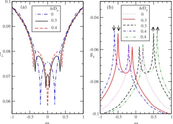
Note that, unlike the equilibrium RG at finite tempera-tures where RG flows are cutoff by temperature T, here in nonequilibrium the RG flows will be cutoff by the decoher-ence rate ⌫, a much lower energy scale than V, ⌫ⰆV. This explains the dip共peak兲 structure in g_⬜共z兲共␻兲 in Figs.1and3. In contrast, the equilibrium RG will lead to approximately frequency-independent couplings 关or “flat” functions g_⬜共␻兲⬇g_⬜,z共␻= 0兲兴. In the absence of field h=0, g_⬜,共z兲共␻兲 show dips共peaks兲 at␻=⫾V/2. In the presence of both bias V and field h, g_⬜共␻兲 shows dips at ␻=⫾V⫾h₂ while gz↑共↓兲

show peaks at ␻= h⫾V/2 共␻= −h⫾V/2兲.20 _{At h = V, two}

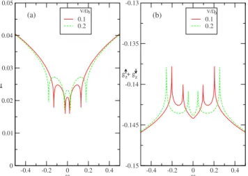
dips of g_⬜共␻兲 at␻=V−h₂ and␻=−V+h₂ merge into a large dip at ␻= 0. Note that in the localized phase the coupling g_⬜共␻→0兲 should get renormalized to zero in the limit of V = 0 and T = 0. As shown in Fig. 4, for a fixed effective magnetic field, the values of g_⬜共␻兲 indeed get further sup-pressed with decreasing bias voltage V, as expected. We use the solutions of the frequency-dependent Kondo couplings g_⬜,z␴共␻兲 to compute occupation number and charge suscep-tibility of the resonance level near the transition.

IV. OCCUPATION NUMBER AND MAGNETIZATION From the mapping, the occupation number of the resonance level nd= d†d is related to the magnetization

of the pseudofermion in the effective Kondo model by Sz= nd− 1/2=

M

2, where M = n↑− n↓= f↑ †_f

↑− f↓†f↓. Since the

oc-cupation number in the dissipative resonance level is related to the pseudospin magnetization in the effective Kondo

-1 -0.5 0 0.5 1 0.06 0.07 0.08 0.09 0.1 -1 -0.5 0 0.5 1 -0.1 -0.08 -0.06 -0.04 ω 0.3 g 0.4 ⊥ g_z 0.3 0.4 h/D0 0.3 0.4 ω h/D₀ 0 0 (a) (b)

FIG. 1.共Color online兲 g_⬜,z共␻兲 versus ␻ 共in unit of D0兲 at the KT

transition for 共a兲 g_⬜共␻兲 and 共b兲 g_z_␴共␻兲. Arrows indicate spin ␴ of the corresponding curve. The bare couplings are g_⬜= −gz= 0.1D0;

bias voltage is fixed at V = 0.4D₀; the effective magnetic fields are fixed at h = 0 , 0.3D0, 0.4D0. Here, D0= 1 for all the figures.

100 102 104 106 108 V/h 10-12 10-8 10-4 Γ 0.1 -0.1 0.075 -0.125 0.05 -0.15 0.025 -0.175 g_z g_⊥

FIG. 2. 共Color online兲 ⌫ versus V/h for different bare Kondo couplings. Here, the bare Kondo couplings g_⬜,zare in units of D0,

and h = 10−9_D 0with D0= 1. -1 -0.5 0 0.5 1 0.01 0.02 0.03 0.04 0.05 -1 -0.5 0 0.5 1 -0.15 -0.145 -0.14 -0.135 -0.13 ω 0.3 g 0.4 ⊥ gz 0.3 0.4 h/D₀ 0.3 0.4 ω h/D0 0 0 (a) (b)

FIG. 3. 共Color online兲 g_⬜,z共␻兲 versus ␻ 共in unit of D0兲 in the

localized phase. for共a兲 g_⬜共␻兲 and 共b兲 g_z_␴共␻兲. Arrows indicate spin ␴ of the corresponding curve. The bare couplings are g⬜= 0.05D0

and g_z= −0.15D₀; bias voltage is fixed at V = 0.4D₀; the effective magnetic fields are fixed at h = 0 , 0.3D0, 0.4D0. Here, D0= 1 for all

(4)

␹␥␥⬘ ⬎,⬜

冉

₋_␻₊␴h 2

冊

册

, ⌺␴⬎共␻兲 =

兺

␥,␥⬘=L,R − i

冋

␹_␥␥⬍,z_⬘

冉

−␻−␴h 2

冊

+␹␥␥⬘ ⬍,⬜

冉

₋_␻₊␴h 2

冊

M =

冕

V−h/2 V+h/2 d␻g_⬜2共␻兲 +

冕

−V−h/2 −V+h/2 d␻g_⬜2共␻兲

冕

−V−h/2 V+h/2 d␻g_⬜2共␻兲 +

冕

−V+h/2 V−h/2 d␻g_⬜2共␻兲 . 共12兲

Note that occupation number n_↑共↓兲can also be determined by the rate equation:20_⌫

↑→↓=⌫↓→↑or n↑A=n↓B, where ⌫↓→↑is

the spin-flip rate of pseudofermion from spin-down to spin-up state.

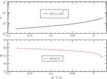
We have calculated the magnetization M共h/V兲 numeri-cally at the KT transition and in the localized phase for both small bias limit V⬇hⰆD0and large bias limit VⰇh where we have fixed h at a small value. First, we demonstrate that the nonequilibrium magnetization M with a fixed h⬇9.6⫻10−8D0for both fixed small共lower panel of Fig.5兲 and large 共upper panel of Fig. 5兲 bias voltages shows a

smooth crossover as a function of g_⬜+ gzacross the KT

tran-sition 共g_⬜+ gz= 0兲, in contrast to a perfect jump in M at the

transition in equilibrium.3

To investigate further the crossover behavior of the mag-netization M, we calculate M as a function of h/V with h being fixed at a small value h⬇1.0⫻10−9_D

0. The result is shown in Fig.6. First, let us examine simple limits from the numerical results. The spin of the quantum dot gets fully polarized M = 1 only when magnetic field h exceeds the bias voltage, hⱖV while for h⬍V the magnetization is reduced due to finite spin-flip decoherence rate. In the extreme large bias limit, VⰇh, we find M gets further suppression.

To gain more understanding of the numerical results, we obtain an analytic approximated form for M共h/V兲 for hⱕV. For V→h, M →1 in the following approximated form:

-0.4 -0.2 0 0.2 0.4 ω 0 0.01 0.02 0.03 0.04 0.05 g 0.1 0.2 -0.4 -0.2 0 0.2 0.4 ω -0.15 -0.145 -0.14 -0.135 -0.13 g + g 0.1 0.2 V/D V/D z z 0 0 (a) (b)

FIG. 4. 共Color online兲 g_⬜,z共␻兲 versus ␻ 共in unit of D₀兲 in the localized phase at a fixed effective magnetic field h = 0.15D0and at

two different bias voltages for共a兲 g_⬜共␻兲 and 共b兲 g_z↑共␻兲+g_z↓共␻兲. The bare couplings are g_⬜= 0.05D0and gz= −0.15D0. Here, D0= 1 for all

(5)

M⬇ h 共V − h兲 g⬜

2_共0兲 g_⬜2共V/2兲+ h

共13兲

while in the large bias limit, V/hⰇ1, we find M共h/V兲 has the following approximated form:

M⬇ hg⬜ 2_共V/2兲 共V − h兲

冋

␲ 4g⬜ 2_{共0兲 +}

冉

_{1 −}␲ 4

冊

g⬜ 2

冉

V − h 2

冊

册

+ hg⬜ 2_共V/2兲 . 共14兲 Here, we have treated g_⬜共␻兲2 _within _the _interval −V−h₂ ⬍␻⬍V−h₂ as a semiellipse. From Eqs.共13兲 and 共14兲, it

is clear that the behavior of the magnetization M共h/V兲 de-pend sensitively on the dip-peak structure in g_⬜共␻兲, espe-cially on the ratio g_⬜共0兲/g_⬜共V/2兲, and g_⬜共V−h₂ 兲/g_⬜共V/2兲. In general, the analytical approximated forms for g_⬜共␻兲 at ␻= 0 ,V₂,V−h₂ are rather complex. Nevertheless, the values of g_⬜共␻兲 at these specific values of␻can be obtained numeri-cally共see, for example, Fig. 7兲.

In the extremely large bias limit, h/V→0, M is well ap-proximated by12 M⬇ hg⬜ 2_共V/2兲 V

冋

␲ 4g⬜ 2_{共0兲 +}

冉

_{1 −}␲ 4

冊

g⬜ 2

冉

V 2

冊

册

. 共15兲

In this limit, the explicit voltage dependence of g_⬜,cr共␻= 0 , V/2兲 at the KT transition are given by12

g_⬜,cr共␻= 0兲 ⬇ 1 2 ln共D/V兲,

g_⬜,cr共␻= V/2兲 ⬇ 1/ln

冉

D 2

⌫V

冊

, 共16兲

Similarly, g_⬜共␻= 0 , V/2兲locin the localized phase take the

following forms: g_⬜,loc共␻= 0兲 − g_⬜ ⬇ A 2c

冋

冉

V D0

冊

2c

冑

c2+ A2

冉

V D0

冊

4c −

冑

A2+ c2

册

+B c

V D0

冊

2c

册

, 共17兲 -0.2 -0.15 -0.1 -0.05 0 10-4 10-3 10-2 10-1 M h/V=1.1x10 -0.2 -0.15 -0.1 -0.05 0 0.5 0.6 0.7 0.8 0.9 M h/V=0.73 -3 z ⊥ g + g

FIG. 5. 共Color online兲 Nonequilibrium magnetization M in the effective Kondo model at fixed h⬇9.6⫻10−8_D

0 and fixed bias

voltage V共small bias with h/V⬇0.73 for lower panel and large bias with h/V⬇1.1⫻10−3 _{for upper panel}_{兲 versus the initial 共bare兲}

Kondo couplings g_⬜+ gzacross the KT transition between the de-localized phase共g_⬜+ g_z⬎0兲 and the localized phase 共g_⬜+ g_z⬍0兲. Here, the bare Kondo couplings g_⬜,z are in units of D0 with D₀= 1. 0.2 0.4 0.6 0.8 1 h/V 0 0.2 0.4 0.6 0.8 1 M (0.025, -0.175) (0.075, -0.125) (0.1, -0.1) (g , g )_⊥ _z

FIG. 6.共Color online兲 Nonequilibrium magnetization M共h/V兲 in the effective Kondo model at the KT transition and in the localized phase. Here, the bare Kondo couplings g_⬜,zare in units of D0, and h = 10−9_D 0with D0= 1. 10-4 10-3 10-2 10-1 100 h/V 0 10 20 30 40 g (0)/ g (V /2) 0.1_{0.075 -0.125}-0.1 0.05 -0.15 0.025 -0.175 ⊥ ⊥ ⊥ g g_z

FIG. 7. 共Color online兲 g_⬜共␻=0兲/g_⬜共␻=V/2兲 versus h/V at the KT transition and in the localized phase. Here, the bare Kondo couplings g_⬜,zare in units of D0, and h = 10−9D0with D0= 1.

(6)

g_⬜,loc共␻= V/2兲 − g_⬜ ⬇ A 2c

冋

冉

V D0

冊

2c

冑

c2+ A2

冉

V D0

冊

4c −

冑

A2+ c2

册

+ B 2c

V D0

冊

2c

册

, 共18兲 where D=e1/共2g⬜兲_, _{A =}g⬜ 2 + cg_⬜ c+兩gz兩, and B = AV c _with

c =

冑

gz2− g_⬜2. Here, we have neglected the subleading terms in

Eqs.共17兲 and 共18兲 which depend logarithmically on V/D0. We first look at the behavior of M共h/V兲 at the KT transi-tion. At a general level one might expect the nonequilibrium magnetization M共h/V兲 at T=0 in the delocalized phase be-have in a similar way as the equilibrium thermal magnetiza-tion M共h/T兲=tanhh

2T with T being replaced by V, leading to linear behavior in h/T at high temperatures. In equilibrium and at finite temperatures, it has been shown that the mag-netization of a closely related model—a resonance level with Ohmic dissipation—exhibits linear behavior in h/T at the KT transition. It is clear from Eq.共15兲 that the magnetization

M共h/V兲 in the equilibrium form based on the “flat approxi-mation”关g_⬜共␻兲⬇g_⬜共␻= 0兲兴 always predicts a linear behav-ior in h/V. At the KT transition, we find the nonequilibrium magnetization M共h/V兲 for h⬇V also shows linear behavior, M⬇h/V. This can be understood from Eq. 共13兲 as at the KT

transition g_⬜共0兲/g_⬜共V/2兲⬇1 for V⬇hⰆD0. The Curie-law 共linear兲 behavior in M共h/V兲 here is reminiscent of the equi-librium thermal magnetization of a free spin in the high-temperature regime. However, at the large bias voltages, VⰇh, we find a logarithmic correction to this linear behavior in M at the KT transition due to the nonequilibrium effect,

M⬇ h V 1

冉

1 −␲ 4

冊

+ ␲ 16

冢

lnD 2 ⌫V lnD V

冣

2. 共19兲

This logarithmic suppression can be understood from Eq. 共15兲 as in this case g_⬜共␻= 0兲关g_⬜共␻= V/2兲兴 becomes peak 共dip兲 and the ratio satisfies g⬜共V/2兲/g⬜共0兲⬍1. We now dis-cuss M共h/V兲 in the localized phase. First, in the limit of small bias, V⬇hⰆD0, as the system gets deeper in the localized phase, M共h/V兲 approaches to fully polarization M = 1 more rapidly than that at the KT transition. This is expected as the system gets deeper in the localized phase, the spin is more easily polarized upon applying a magnetic field. This behavior can also be explained from Eq.共13兲 as in the

localized phase the ratio g_⬜共0兲/g_⬜共V/2兲⬍1, and it only gets smaller as the system gets deeper in the localized phase. In fact, the same qualitative behavior is seen in a closely related Bose-Fermi Kondo model3 _{which shows the KT transition}

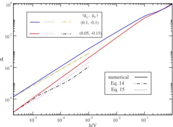
between the Kondo and local-moment ground states. In the large bias limit VⰇh, however, M deviates from the linear behavior due to nonequilibrium effects. The correction of M

to linear behavior is dominated by the ratio g_⬜共0兲/g_⬜共V/2兲 via Eq. 共15兲, where g_⬜共␻兲 shows deeper dips at␻=⫾V/2, making g_⬜共0兲/g_⬜共V/2兲 to rapidly increase with decreasing h/V 共see Fig.7兲. This gives rise to a further suppression of

M at large bias voltages compared to that at the KT transition 共see Fig.8兲.

Note that from Figs.6 and8, as the system goes deeper into the localized phase共or with decrease in g_⬜+ gz⬍0兲, we

find M for a fixed hⰆD0 increases for a fixed small bias voltage 共0.4⬍h/V⬍1兲 while it decreases for a fixed large bias voltage共h/VⰆ1兲. This is in perfect agreement with the crossover behavior for M shown in Fig.5.

Notice that the linear behavior of M共h/V兲⬇h/V is ex-pected in purely asymmetric gLR⬎0=gLL/RR but isotropic

共gLL/RR/LR,⬜= gLL/RR/LR,z兲 Kondo model.20 In a symmetric

Kondo model with g = gLL= gRR= gLR, the nonequilibrium

magnetization M共h/V兲 acquires an additional positive loga-rithmic corrections M⬇共2h/V兲共1+2g ln兩V/h兩兲.19,20 _{In the}

present case, however, the deviation from the linear behavior of M共h/V兲 in the large bias limit has a different origin. It comes from the fact that our effective Kondo model is not only asymmetric 共gLL_/RR= 0⬍gLR兲 but also highly

aniso-tropic共g_LR,zⱕ−兩g_LR,_⬜兩兲 at the KT transition and in the local-ized phase. Different corrections to the linear behavior are expected.

V. SUSCEPTIBILITY␹

The nonequilibrium charge susceptibility␹共V兲⬅⳵nd

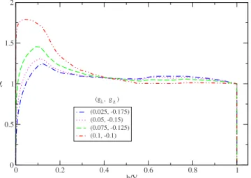
⳵h in the dissipative resonance level is obtained from the spin suscep-tibility␹=⳵M_⳵h in the effective Kondo model by the mapping mentioned above. The susceptibility ␹ of a Kondo dot in equilibrium at finite temperatures is given by the Curie’s law ␹=_2T1. However, in our highly asymmetric and anisotropic Kondo model, we find the nonequilibrium susceptibility de-viates significantly from the Curie law. As shown in Fig.9, at the KT transition, as bias voltage is increased, ␹共V兲 first

10-5 10-4 10-3 10-2 10-1 h/V 10-6 10-4 10-2 100 M (0.1, -0.1) (0.05, -0.15) (g , g )_⊥ z numerical Eq. 14 Eq. 15

FIG. 8.共Color online兲 Nonequilibrium magnetization M共h/V兲 in the effective Kondo model at the KT transition and in the localized phase. The dotted-dashed 共dot兲 lines are results via Eq. 共14兲 and 共15兲. Here, the bare Kondo couplings g_⬜,zare in units of D₀, and

(7)

shows 1/V Curie-law behavior, followed by an increase and a peak around h/V=0.1. In the large bias limit,␹共V兲 gets a logarithmic suppression关see Eq. 共15兲兴,

␹⬇ 1 V 1

冉

1 −␲ 4

冊

+ ␲ 16

冢

lnD 2 ⌫V lnD V

冣

2. 共20兲

Note that the rapid increase in ␹共h/V兲 at the KT transition with decreasing h/V for 0.1⬍h/V⬍0.5 is reminiscent of the spin susceptibility of a nonequilibrium Kondo dot in a mag-netic field where ␹共h/V兲 acquires a logarithmic increase at large bias voltages.20 _{On the other hand, the logarithmic}

de-crease in␹共h/V兲 here at large bias is a direct consequence of the dip structure in g_⬜共␻兲 at the KT transition 关see Eq. 共16兲

and Fig. 10兴.

As the system gets deeper in the localized phase,␹共h/V兲 gets a more pronounced peak at h⬇0.7V. As bias is further increased, ␹共h/V兲 shows a similar trend as that at the KT transition—a peak around h/V=0.1 but smaller magnitudes 共see Fig. 9兲. At large bias voltages, VⰇh, ␹ gets a more severe power-law suppression compared to the slower loga-rithmic decrease at the KT transition 关see Fig.10 and Eqs. 共17兲 and 共18兲兴, ␹⬇ 1 V 1

冉

1 −␲ 4

冊

+ ␲ 4 g_⬜,loc2 共0兲 g_⬜,loc2 共V/2兲 共21兲

with g_⬜,loc共0兲,g_⬜,loc共V/2兲 given by Eqs. 共17兲 and 共18兲. This

comes as a result of further decrease in Kondo coupling g_⬜共␻兲 at␻=⫾V/2 in the localized phase under RG.

We may compare the behavior in ␹共V兲 in our model at large bias voltages with that in different limit of the same model or with different models. In the equilibrium limit V→0 within our model where g_⬜,z共␻兲 can be considered as flat functions over −V+h₂ ⬍␻⬍V+h₂ , g_⬜共␻= 0兲/g_⬜共␻= V/2兲 ⬇1, a perfect Curie-law behavior is expected for␹共V兲. How-ever, for isotropic Kondo model共gLL= gRR= gLR兲 for a simple

quantum dot in Kondo regime and at large bias voltages, ␹共V兲 shows Curie law with positive logarithmic correction, ␹⬇1

V共1+

1 ln_TV

k

兲 with Tkbeing Kondo temperature for a

single-quantum dot. In our dissipative resonance-level model, the suppression in ␹共h/V兲 at large bias voltages at the KT tran-sition and in the localized phase comes from the dips at g_⬜共␻=⫾V/2兲.

VI. DISCUSSIONS AND CONCLUSIONS

Before we conclude, let us discuss the relevance of our results for the transport measurements in nanostructures. First, the nonequilibrium occupation number 共charge on the quantum dot兲 nd共h/V兲=M共h/V兲+1/2 can be detected by the

single-electron transistor 共SET兲 connected to the dot by tun-ing the gate voltage Vgon the dot via eN = VgCgwith Cgbeen

the capacitance between gate and dot,22 _{and the effective}

magnetic field h = Vg− e2/共2Cg兲⬀共N−1/2兲 being the

devia-tions of N from the degeneracy point.3_{Alternatively, the}

av-erage charge on the dot can also be detected by the time-resolved current and conductance measurement of the quantum point-contact capacitively coupled to the dot.23_{At a}

finite bias, instead of a perfect Coulomb step, a smooth crossover behavior for M共h/V兲 is expected near the KT tran-sition. Second, the charge 共impurity兲 susceptibility ␹共h兲=dM /dh can be measured by the capacitance line shape near the charge degeneracy point via the high sensitivity charge sensor in the SET connected to the dot: Cdot= dnd/dVg⬀dnd/dh=␹共h兲.22,24,25We believe in principle

it is possible to generalize the above setup to a dissipative resonant-level dot. We have predicted specific crossover be-haviors for M and ␹ at the transition and in the localized phase. In particular, in the large bias limit h/VⰆ1, we find a logarithmic and a power-law correction in V for M共h/V兲 and ␹共h/V兲 to the Curie-law behavior is predicted at the KT

tran-0 0.2 0.4 0.6 0.8 1 h/V 0 0.5 1 1.5 2 χ (0.025, -0.175) (0.05, -0.15) (0.075, -0.125) (0.1, -0.1) (g , g )⊥ z

FIG. 9. 共Color online兲␹共h/V兲 versus h/V at the KT transition and in the localized phase. Here, the bare Kondo couplings g_⬜,zare in units of D0, and h = 10−9D0with D0= 1.

10-5 10-4 10-3 10-2 10-1 100 h/V 10-1 100 χ (0.025, -0.175) (0.05, -0.15) (0.075, -0.125) (0.1, -0.1) (g , g )_⊥ _z

FIG. 10. 共Color online兲␹共h/V兲 versus h/V at the KT transition and in the localized phase. Here, the bare Kondo couplings g_⬜,zare in units of D₀, and h = 10−9_D

(8)

sition and in the localized phase, respectively. These non-equilibrium crossover behaviors at finite bias voltages near the phase transition are fundamentally distinct from those in equilibrium at finite temperatures.

In conclusion, we have investigated the nonequilibrium occupation and charge susceptibility of a dissipative reso-nance level with energy h. For h = 0, the system exhibits the Kosterlitz-Thouless-type quantum transition between a delo-calized phase at small dissipation strength and a lodelo-calized phase with large dissipation. We first mapped our problem onto an effective nonequilibrium anisotropic Kondo model in the presence of a magnetic field h. The occupation number and charge susceptibility correspond to magnetization M and susceptibility ␹ of the pseudospin in the effective Kondo model, respectively. By nonequilibrium RG approach, we solved for the frequency-dependent effective Kondo cou-plings and calculated magnetization M共h/V兲 and ␹共h/V兲 at finite bias voltages. We demonstrate the smearing of the KT transition in the nonequilibrium magnetization M at a fixed h as a function of the effective anisotropic Kondo couplings for both small bias and large bias voltages as it exhibits a smooth crossover at the KT transition, in contrast to a perfect

jump in M at the transition in equilibrium. For small bias V and effective field h and h⬇V, we find the magnetization M共h/V兲 at the KT transition shows linear behavior in h/V while in the localized phase M increases more rapidly with V approaching h from above, consistent with the behavior of the equilibrium magnetization in the localized phase at finite temperatures. In the large bias limit VⰇh, however, we find corrections to equilibrium Curie-law behavior in M due to nonequilibrium effects. At the KT transition, the corrections are logarithmic, in V/D, while in the localized phase they are power law in V/D0. Our results have direct relevance for nonequilibrium charge fluctuations in quantum dots, and it is of great interest to investigate further these nonequilibrium crossovers in future experiments.

ACKNOWLEDGMENTS

We are grateful for the helpful discussions with P. Wöelfle. This work is supported by the NSC under Grants No. 98-2918-I-009-06 and No. 98-2112-M-009-010-MY3, the MOE-ATU program, and the NCTS of Taiwan, R.O.C. 共C.H.C.兲.

1_{S. Sachdev, Quantum Phase Transitions}_{共Cambridge University}

Press, Cambridge, England, 2000兲.

2_{S. L. Sondhi, S. M. Girvin, J. P. Carini, and D. Shahar,} _Rev.

Mod. Phys. 69, 315共1997兲.

3_{K. Le Hur,}_{Phys. Rev. Lett. 92, 196804}_共2004兲_{; M.-R. Li, K. Le}

Hur, and W. Hofstetter,ibid. 95, 086406共2005兲.

4_{K. Le Hur and M.-R. Li,}_{Phys. Rev. B 72, 073305}_共2005兲. 5_{P. Cedraschi and M. Büttiker,}_{Ann. Phys.}_{共N.Y.兲 289, 1 共2001兲.} 6_{A. Furusaki and K. A. Matveev,} _{Phys. Rev. Lett. 88, 226404}

共2002兲.

7_{L. Borda, G. Zarand, and D. Goldhaber-Gordon,}

arXiv:cond-mat/0602019共unpublished兲.

8_{G. Zarand, C. H. Chung, P. Simon, and M. Vojta,} _{Phys. Rev.}

Lett. 97, 166802共2006兲.

9_{G. Refael, E. Demler, Y. Oreg, and D. S. Fisher,} _{Phys. Rev. B} 75, 014522共2007兲.

10_{K. Moon,}_{Int. J. Mod. Phys. B 19, 471}_共2005兲.

11_{J. Gilmore and R. McKenzie, J. Phys. C 11, 2965}_共1999兲. 12_{C. H. Chung, K. Le Hur, M. Vojta, and P. Wölfle,} _{Phys. Rev.}

Lett. 102, 216803共2009兲.

13_{D. E. Feldman,}_{Phys. Rev. Lett. 95, 177201}_共2005兲.

14_{A. Mitra, S. Takei, Y. B. Kim, and A. J. Millis,}_{Phys. Rev. Lett.} 97, 236808共2006兲; A. Mitra and A. J. Millis,Phys. Rev. B 77, 220404共R兲共2008兲; A. Mitra, I. Aleiner, and A. J. Millis,ibid.

69, 245302共2004兲.

15_{A. O. Caldeira and A. J. Leggett,}_{Ann. Phys.} _{共N.Y.兲 149, 374}

共1983兲; A. J. Leggett, S. Chakravarty, A. T. Dorsey, M. P. A.

Fisher, A. Garg, and W. Zwerger,Rev. Mod. Phys. 59, 1共1987兲.

16_{C.-H. Chung, M. T. Glossop, L. Fritz, M. Kircan, K. Ingersent,}

and M. Vojta,Phys. Rev. B 76, 235103共2007兲.

17_{M. T. Glossop and K. Ingersent,} _{Phys. Rev. B 75, 104410}

共2007兲; M. T. Glossop, N. Khoshkhou, and K. Ingersent,Physica B 403, 1303 共2008兲; M. Cheng, M. T. Glossop, and K. In-gersent,Phys. Rev. B 80, 165113共2009兲.

18_{R. Bulla, N.-H. Tong, and M. Vojta,}_{Phys. Rev. Lett. 91, 170601}

共2003兲.

19_{J. Paaske, A. Rosch, and P. Wölfle,} _{Phys. Rev. B 69, 155330}

共2004兲.

20_{A. Rosch, J. Paaske, J. Kroha, and P. Wolfle,}_{Phys. Rev. Lett. 90,}

076804共2003兲; A. Rosch, J. Paaske, J. Kroha, and P. Wöffle,J. Phys. Soc. Jpn. 74, 118共2005兲.

21_{K. A. Matveev,}_{Phys. Rev. B 51, 1743}_共1995兲.

22_{D. Berman, N. B. Zhitenev, R. C. Ashoori, H. I. Smith, and M.}

R. Melloch, J. Vac. Sci. Technol. B 15, 2844共1997兲; D. Ber-man, N. B. Zhitenev, R. C. Ashoori, and M. Shayegan, Phys. Rev. Lett. 82, 161共1999兲; K. W. Lehnert, B. A. Turek, K. Bladh, L. F. Spietz, D. Gunnarsson, P. Delsing, and R. J. Schoelkopf,

ibid. 91, 106801共2003兲.

23_{S. Gustavsson, R. Leturcq, M. Studer, I. Shorubalko, T. Ihn, K.}

Ensslin, D. C. Driscoll, and A. C. Gossard,Surf. Sci. Rep. 64, 191共2009兲.

24_{K. Le Hur and G. Seelig,}_{Phys. Rev. B 65, 165338}_共2002兲. 25_{C. J. Bolech and N. Shah,}_{Phys. Rev. Lett. 95, 036801}_共2005兲.