行政院國家科學委員會專題研究計畫 成果報告
802.11e/802.16 閘道於點對點/網狀/轉傳模式下之服務品
質提供
研究成果報告(精簡版)
計 畫 類 別 : 個別型
計 畫 編 號 : NSC 95-2221-E-004-005-
執 行 期 間 : 95 年 08 月 01 日至 96 年 07 月 31 日
執 行 單 位 : 國立政治大學資訊科學系
計 畫 主 持 人 : 蔡子傑
計畫參與人員: 碩士班研究生-兼任助理:王川耘、陳彥賓、張志華
報 告 附 件 : 出席國際會議研究心得報告及發表論文
處 理 方 式 : 本計畫可公開查詢
中 華 民 國 96 年 10 月 31 日
行政院國家科學委員會補助專題研究計畫成果報告
802.11e/802.16 閘道於點對點/網狀/轉傳模式下之服務品質提供
計畫類別:■ 個別型計畫 □ 整合型計畫
計畫編號:NSC 95-2221-E-004-005
執行期間: 95 年 8 月 1 日至 96 年 7 月 31 日
計畫主持人:蔡子傑
共同主持人:
計畫參與人員: 王川耘、陳彥賓、張志華
成果報告類型(依經費核定清單規定繳交):■精簡報告 □完整報告
本成果報告包括以下應繳交之附件:
□赴國外出差或研習心得報告一份
□赴大陸地區出差或研習心得報告一份
■出席國際學術會議心得報告及發表之論文各一份
□國際合作研究計畫國外研究報告書一份
處理方式:除產學合作研究計畫、提升產業技術及人才培育研究計畫、
列管計畫及下列情形者外,得立即公開查詢
□涉及專利或其他智慧財產權,□一年□二年後可公開查詢
執行單位:國立政治大學 資訊科學系
中 華 民 國 96 年 10 月 31 日
行政院國家科學委員會專題研究計畫成果報告
802.11e/802.16 閘道於點對點/網狀/轉傳模式下之服務品質提供
計畫編號:NSC 95-2221-E-004-005
執行期限:95 年 8 月 1 日至 96 年 7 月 31 日
主持人:蔡子傑 國立政治大學 資訊科學系
計畫參與人員:王川耘、陳彥賓、張志華
此 成 果 報 告 為 三 篇 論 文 的 集 節 : [ 1 ] T z u - C h i eh Ts a i a n d C h u a n - Y i n W a n g , "Routing and Admission Control in IEEE 802.16 Distributed Mesh Networks", in IEEE Fourth International Conference on Wireless and Optical Communications Networks" (WOCN 2007), July 2, 3 and 4, 2007, Singapore. (IEEE Catalog Number: 07EX 1696, ISBN: 1-4244-1005-3, Library of Congress: 2007920880), (Engineering Index (EI) a n d E I C o m p e n d e x ) . [2] Tzu-Chieh Tsai,Chen Yan-Bin, "Modeling the Distributed Scheduler of IEEE 802.16 Mesh Mode", in 2006 National Symposim on Telecommunications, K a o h s i u n g , T a i w a n , D e c 0 1 ~ 0 2 , 2 0 0 6 . [3] Tzu-Chieh Tsai, Chih-Hua Chang, “QoS Guarantee for IEEE 802.16 Integrating with 8 0 2 . 1 1 e ” , p r e p a r e d t o s u b m i s s i o n .首先我們先整理摘錄此三篇論文在本計畫中的關聯 度與重要成果,後附上完整論文內容供參考。其中 第三篇還未投稿,暫不附全文,請見諒。
另外,已發表的先前論文有兩篇:
[4] Tzu-Chieh Tsai, and Ming-Ju Wu, "An Analytical Model for IEEE 802.11e EDCA", in IEEE 2005 International Conference on Communications (ICC 2005 Wireless Networking), 16-20 May, 2005, Seoul, Korea. pp. 3474 - 3478.(ISSN: 0536-1486, EI)
[5] Tzu-Chieh Tsai, Chi-Hong Jiang, and Chuang-Yin Wang, "CAC and Packet Scheduling Using Token Bucket for IEEE 802.16 Networks", in Journal of Communications (JCM, ISSN 1796-2021), Volume : 1 Issue : 2, May, 2006. Page(s): 30-37. Academy Publisher.
一、Abstract
本研究主要研究主題為服務品質(Quality of Service, QoS),以 802.16 與 802.11e 為主,探討 802.16 的三種傳輸模式、與 802.11e 的服務品質 對應與保證該如何達成,還有如何對封包做排程的 動作;除此之外,第一層調變技術的選擇與第三層 的繞徑協定也部分包括在本研究計畫中,以期讓使 用者在上網時得到更好的服務品質。 本 研 究 對 現 有 無 線 網 路 架 構 做 了 少 許 的 修 改,而得到一個類似於現有網路架構,但卻更富有 挑戰性且成本更低、更方便的新網路架構:使用者 的 mobile devices 以 802.11e 的 網 路 卡 連 上 Access Point(AP),而 AP 後端以 802.16 連上網際 網路,這樣的 AP,我們稱為 802.11e/802.16 閘道 器。在這樣的環境中,使用者的移動性(mobility) 以及可能需要交遞(handoff)的問題,都可以由現 有的 802.11 相關的處理方法來解決,由於關於這 個主題的研究已經不勝枚舉,本研究在這部份將不 多作著墨,而將專注於 802.16 相關議題與傳輸模 式的研究。 在目前的 802.16-2004 版本中,定義了兩種 傳輸模式,分別是:點對多點(PMP)與網狀(mesh)兩 種,兩種模式各有優缺點,而我們預計會有新的傳 輸模式:轉傳模式(relay)將結合兩者的優點,並 會被廣泛的使用。為了本研究的一致性與完整性, 本研究將對二種模式做個別深入的探討。 上述的二種傳輸模式,都將在我們的閘道器 後端選用,因此分別產生了二種如何提供服務品質 的問題,我們將對二種模式分別提出如何對應服務 品質與保證的方法。 本研究將對所提出的網路架構,提出一套由 下而上,跨越 OSI 標準中的第一、二、三層的設
計,其中在第二層,包括了 802.11e 以及 802.16 的所有可能模式,結合了目前炙手可熱的兩種科 技:WLAN、WiMax,期望提供更好的服務品質與新的 網路使用經驗給使用者,並成就一深度、廣度兼具 的完整性研究。 關鍵詞:服務品質、802.11e、802.16、 點對多點、 網狀、轉傳模式 二、緣由與目的、結果與討論
在 802.11e/802.16 Gateway 之 QoS 研
究,分為幾個部份。
z
802.11e QoS
z
802.16 QoS for PMP Mode
z
802.16 QoS for Mesh Mode
z
802.11e/802.16 Integration
其中 802.11e QoS 的研究,之前就已有成
果 發 表 在 [4]. 在 那 篇 論 文 中 , 我 們 用
Markov Chain 去 model 各個 Access Category
的 channel access 情形,進而求出各個服務
等 級 的 MAC delay , 針 對 在 不 同 的 loading
下 。 如 此 可 以 供 作 CAC(Call admission
control)的依據,而達成 QoS 的要求。
而 802.16 QoS for PMP Mode 的研究,也
是之前我們就有成果發表在[5]. 在那篇論文
中 , 我 們 用 token bucket 的方 式,去控 制
rtPS 等級的 traffic,進而能有效預估在符合
delay 要求條件下所需要的頻寬。藉此也發展
出 scheduling algorithm 以及 CAC。在這篇
論文,我們的 scheduling 與 CAC 特別設計
下,任何等級的服務不會有 starvation 的情
況。另外,我們也針對 Poisson traffic,利
用 Markov Chain 分析,在 token bucket 模式
下,該如何管理這些參數,以致於最有效率的
達到 QoS。
接續[5]的 QoS 研究經驗,我們繼續研究如
何擴充我們的作法到 Mesh Mode。首先, 必
需瞭解 Mesh Mode 的運作模式與 PMP Mode 有
何不同。我們發現在 access 方式大大不同,
所以會多增加 access delay 的部份。因此我
們 研 究 了 這 個 部份 在[2]。 而 token bucket
based CAC and scheduling for Mesh Mode
則在[1]。最後我們再將 802.11e 的部份以及
802.16 作整合的 delay 與 CAC 的研究則在
[3]。
接下來,我們就分別摘錄[1][2][3]的重要
成果。完整論文則附於後面。
1. "Routing and Admission Control in IEEE 802.16 Distributed Mesh Networks"
1.1 Abstract
QoS provisioning in wireless mesh network has been known to be a challenging issue. In this paper, we propose a fixed routing metric (SWEB) that is well-suited in IEEE 802.16 distributed, coordinated mesh mode. Also, an admission control algorithm (TAC) which utilizes the token bucket mechanism is proposed. The token bucket is used for controlling the traffic patterns for easy estimating the bandwidth used by a connection. In the TAC algorithm, we apply the bandwidth estimation by taking the hop count and delay requirements of real-time traffics into account. TAC is designed to guarantee the delay requirements of real-time traffics, and avoid the starvations of low priority traffics. With the proposed routing metrics, the admission control algorithm and the inherent QoS support of the IEEE 802.16 mesh mode, a QoS-enabled environment can be established. Finally, extensive simulations are carried out to validate our algorithms. 1.2 Main Results
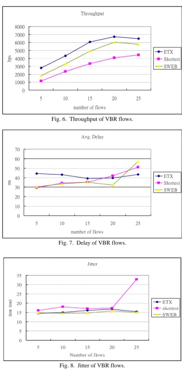
The proposed SWEB is compared with the ETX and the shortest path. The performance and delay of VBR traffics are compared across all three different metrics. The performance is given in figure 1. And figure 2 shows the delay.
As shown in the figure 1 and 2, when number of flows is reaching 25, some VBR flows are preempted by CBR flows. By simulation results, we claim that SWEB is a compromise of delay and throughput. But in figure 3, we can find that SWEB has best performance in jitter of real-time packets.
Throughput 0 1000 2000 3000 4000 5000 6000 7000 8000 5 10 15 20 25 number of flows bps ETX Shortest SWEB
Fig. 1. Throughput of VBR flows.
Avg. Delay 0 10 20 30 40 50 60 70 5 10 15 20 25 number of flows ms ETX Shortest SWEB
Fig. 2. Delay of VBR flows. Jitter 0 5 10 15 20 25 30 35 5 10 15 20 25 Number of flows ti m e ( m s) ETX shortest SWEB
Fig. 3. Jitter of VBR flows.
In TAC algorithm, the minimum usage of each traffic class must be set. In the simulations, the
CBR_min, VBR_min and BE_min are set as 10, 40 and
75 timeslots, respectively. Also, the parameters of token bucket are shown in table III.
We compare the throughput in figure 4 and figure 5. In figure 4, BE traffics suffers from preemption from higher priority traffic class, therefore, receiving low throughput when network is heavily-loaded. By applying the CAC algorithm in figure 5, the BE flows has the guaranteed throughput by setting the minimum usage. The preemption occurs only in down-graded flows. throughput 0 1000 2000 3000 4000 5000 6000 7000 8000 5 10 15 20 25 number of flows bps CBR VBR BE total
Fig. 4. Throughput for the original IEEE 802.16 mesh mode.
(TAC) throughput 0 1000 2000 3000 4000 5000 6000 7000 8000 5 10 15 20 25 number of flows bp s CBR VBR BE total
Fig. 5. Throughput when TAC is applied.
2. "Modeling the Distributed Scheduler of IEEE
802.16 Mesh Mode" 2.1 Abstract
The IEEE 802.16 standard is a protocol for wireless metropolitan networks. IEEE 802.16 MAC protocol supports both of PMP (point to multipoint) and Mesh mode. In the mesh mode, all nodes are organized in a similar ad-hoc fashion and calculate their next transmission time based on the scheduling information performed in the control subframe. Each node has to compete with each other to win the time slots of opportunities for the subsequent advertisement of the scheduling messages to its neighbors. This behavior does not depend on all of past history. In other words, it is a "Time Homogeneous" and suitable for being modeled by stochastic process. In this study, we will model this scheduling behavior by queuing process, and apply the Markov Chain to estimate its average delay time which a node keep waiting until it win the competition.
2.2 Main Results
We validate our model by the following. The transmission behavior is simulated by our C code. The mathematic evaluations are computed by the MATLAB 7.0.
The result is shown as Fig.6. With this figure, it shows our mathematical model approaches the simulation result. 2~20 Nodes 0 20 40 60 80 100 120 2 4 6 8 10 12 14 16 18 20 Number of nodes op po rtu ni tie s( tim e sl ot ) sim math p=0.5
Fig. 6: The delay time of opportunities between simulation and mathematic model
The error rate is shown as Fig.7. It shows the error is under 10% while the nodes of number between 2 to 20.
2~20 Node Error Rate 0 10 20 30 40 50 60 70 80 90 100 2 4 6 8 10 12 14 16 18 20 Number of nodes E rro r ra te (1 00 % ) Error rate(%)
Fig. 7: The error rate between simulation and mathematic model
3. "QoS Guarantee for IEEE 802.16 Integrating with
802.11e" 3.1 Abstract
IEEE 802.16 and 802.11e both provide Quality of Service (QoS), but the MAC of betweens is different. Ensuring the QoS guarantee, we use a Markov Chain model to analyze the 802.11e EDCA delay time under variance number of connections. Therefore, we can employ a CAC mechanism constraining the number of connections to guarantee the delay requirement. Further, considering the delay requirement and the bandwidth, we use a Token Bucket mechanism to throttle the traffic output that ensures the delay and bandwidth to be satisfied. And our Token Bucket mechanism can tune the token rate automatically by bandwidth requirement. Finally, we use the Packet Drop mechanism to improve throughput.
3.2 Main Results
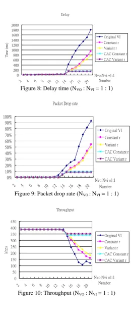
We validate our methos through comparing delay, throughput and packet drop rate with the simulator Qualnet. The VI (rtPS) delay is what we mainly concern about. Therefore, we just show the VI (rtPS) delay time and the result.
There are five lines we compare with. Original VI means we just run the scenario without any change in protocol. Constant r represents using Token Bucket mechanism but without tuning the token rate r. Variant r expresses using Token Bucket mechanism and it will tune the token rate r. CAC Constant r and CAC Variant r are similar to Constant r and Variant r but with CAC mechanism. Expect the Original VI, otherwise with our packet drop mechanism. The simulation result is as Figure 8, Figure 9, and Figure 10.
Delay 0 200 400 600 800 1000 1200 1400 1600 1800 2000 2 4 6 8 10 12 14 16 18 20 Nvo:Nvi =1:1 Number Tim e (m s) Original VI Constant r Variant r CAC Constant r CAC Variant r
Figure 8: Delay time (NVO : NVI = 1 : 1)
Packet Drop rate
0% 10% 20% 30% 40% 50% 60% 70% 80% 90% 100% 2 4 6 8 10 12 14 16 18 20 Nvo:Nvi =1:1 Number Original VI Constant r Variant r CAC Constant r CAC Variant r
Figure 9: Packet drop rate (NVO : NVI = 1 : 1)
Throughput 0 50 100 150 200 250 300 350 400 450 2 4 6 8 10 12 14 16 18 20 Nvo:Nvi =1:1 Number kbps Original VI Constant r Variant r CAC Constant r CAC Variant r Figure 10: Throughput (NVO : NVI = 1 : 1) 三、計畫成果自評 本計畫的 scope 相當大,但是我們先前已 有 很 紮 實 的 研 究 經 驗 與 成 果 。 因 此 不 論 在 802.11e 的 QoS 或 802.16 以 token bucket based 的 QoS 都可循經驗再作進一步的擴充與 整合。
這個計畫花較多的時間是在研讀 802.16 Mesh mode 的 draft。由於是較新的文件,一些 其他輔助資料較欠缺,不過經過一番努力,還 是把它完成了。我想這個部份的成果應可作為 其 他 機 構 在 研 究 這 個 主 題 時,一個很好的參 考。
另外,我們在整合 802.11e 與 802.16 時, 用 Markov Chain 去 model delay analysis,碰 到一些瓶頸,因為不同的架構下,要整合成一 套相容的 QoS 管理機制,本就有困難度。不 過,我們還是把它達成了,雖不盡完美但尚可 接受。日後可供 WiMAX 業者與 WiFi HotSpot 業 者 結 盟 一 個 非 常 好 的 管 理 平 台 作 參 考 。
可供推廣之研發成果資料表
■ 可申請專利 ■ 可技術移轉日期:96 年 10 月 31 日
國科會補助計畫
計畫名稱:802.11e/802.16 閘道於點對點/網狀/轉傳模式下之服務品質提供 計畫主持人: 蔡子傑 計畫編號: NSC 95-2221-E-004-005 學門領域:資訊技術/創作名稱 Routing and Admission Control in IEEE 802.16
Distributed Mesh Networks
發明人/創作人
蔡子傑,王川耘 中文:我們 針對 IEEE 802.16 協調分散式之網狀網路提出一允入控
制之演算法。在此類網路中,控制子訊框交換各站台之排程訊
息,並預留資料子訊框之時槽作為實際資料傳輸之用。我們利用
令牌桶機制來控制網路訊流之流量特徵,如此可簡單的估計各訊
流所需之頻寬。我們使用了所提出的頻寬估計方法,並一起考慮
各訊流之跳接數與延遲時間之需求,提出的允入控制演算法能夠
保證即時性串流之延遲時間需求,且可避免低等級訊流發生飢餓
情形。模擬結果顯示,所提出的允入控制方法可以有效的把超過
延遲時間需求之即時性訊流封包數目降低,並且低等級訊流在網
路負載大時仍然可以存取頻道。
技術說明
英文:
We propose a routing metric (SWEB: Shortest-Widest Efficient
Bandwidth) and an admission control (TAC: Token bucket-based
Admission Control) algorithm under IEEE 802.16 coordinated,
distributed mesh networks. In such network architectures, all
scheduling messages are exchanged in the control subframes to reserve
the timeslots in data subframes for the actual data transmissions. The
token bucket mechanism is utilized to control the traffic pattern for
easily estimating the bandwidth of a connection. We apply the
bandwidth estimation and take the hop count and delay requirements
into consideration. TAC is designed to guarantee the delay
requirements of the real-time traffic flows, and avoid the starvation of
the low priority ones. Simulation results show that TAC algorithm can
effectively reduce the number of real-time packets that exceed the
delay requirements and low priority flows still can access the channel
when the network is heavily-loaded.
可利用之產業
及
可開發之產品
相關 802.16 的產業 附件二
技術特點
利用 token bucket 來管理與控制頻寬,並提出 CAC 與 scheduling 機制來達成 QoS 的要求。
推廣及運用的價值
WiMAX 的執照已陸續在發放,業者也會建置越來越多的基地台。
然而不管是 PMP 或 Mesh Mode,QoS 的管理是 WiMAX 相當重要
的課題。因此本研究成果可供業者一個很重要的參考依據。
※ 1.每項研發成果請填寫一式二份,一份隨成果報告送繳本會,一份送 貴單位研發成果推廣單
位(如技術移轉中心)。
※ 2.本項研發成果若尚未申請專利,請勿揭露可申請專利之主要內容。
附論
已發表之論文全文
[1] Tzu-Chieh Tsai and Chuan-Yin Wang, "Routing and Admission Control in IEEE 802.16 Distributed Mesh Networks", in IEEE Fourth International Conference on Wireless and Optical Communications Networks" (WOCN 2007), July 2, 3 and 4, 2007, Singapore. (IEEE Catalog Number: 07EX1696, ISBN: 1-4244-1005-3, Library of Congress: 2007920880), (Engineering Index (EI) and EI Compendex). [2] Tzu-Chieh Tsai,Chen Yan-Bin, "Modeling the Distributed Scheduler of IEEE 802.16 Mesh Mode", in 2 0 0 6 N a t i o n a l S y m p o s i m o n T e l e c o m m u n i c a t i o n s , K a o h s i u n g , T a i w a n , D e c 0 1 ~ 0 2 , 2 0 0 6 .
1
Abstract—QoS provisioning in wireless mesh network has been
known to be a challenging issue. In this paper, we propose a fixed routing metric (SWEB) that is well-suited in IEEE 802.16 distributed, coordinated mesh mode. Also, an admission control algorithm (TAC) which utilizes the token bucket mechanism is proposed. The token bucket is used for controlling the traffic patterns for easy estimating the bandwidth used by a connection. In the TAC algorithm, we apply the bandwidth estimation by taking the hop count and delay requirements of real-time traffics into account. TAC is designed to guarantee the delay requirements of real-time traffics, and avoid the starvations of low priority traffics. With the proposed routing metrics, the admission control algorithm and the inherent QoS support of the IEEE 802.16 mesh mode, a QoS-enabled environment can be established. Finally, extensive simulations are carried out to validate our algorithms.
Index Terms—IEEE 802.16, wireless mesh networks, WiMAX
I. INTRODUCTION
S wireless technology evolves, IEEE 802.16[1], or WiMAX (Worldwide Interoperability for Microwave Access), appears to be a great competitor to IEEE 802.11 or 3G networks for its wide coverage and high data rate. In the IEEE 802.16 standards, meshing functionality is included as an optional mode. We propose a simple routing metrics called Shortest Widest Effective Bandwidth (SWEB) and a Token bucket-based Admission Control (TAC) in the IEEE 802.16 mesh networks.
IEEE 802.16 is a standard that aims at the use of wireless metropolitan area network (WMAN). Two modes are defined in the standard: PMP (Point to Multi-Point) and mesh mode. In PMP mode, the network architecture is similar to the cellular network. That is, one base station (BS) is responsible for all its subscriber stations (SS). The transmission can occur only between BS and SS. In mesh mode, the networks architecture is similar to the ad-hoc networks. In other words, each SS can be a source node and a router at the same time. The transmission can occur between any two stations in the network.
IEEE 802.16 mesh network is time-slotted. Connections must reserve timeslots in advance for the actual transmissions. As IEEE 802.16 is mostly used as the network backhaul, the network traffics mostly occur between the BS and SS.
Therefore, with appropriate routing algorithm, the topology can be reduced into a routing tree. QoS of a connection along the path from the source station to the base station can be provided. The remaining parts of this paper are organized as follows: Section II gives the background knowledge of token bucket mechanism and details of IEEE 802.16 mesh mode. Section III includes the related works. In section IV and V, the SWEB and TAC are proposed. Simulation results are given in section VI. Finally, we conclude this paper in section VII.
II. BACKGROUND
A. Token Bucket mechanism
Token bucket is a mechanism that controls the network traffic rate injecting to networks. It works well for the “bursty” traffics. Token bucket mechanism needs two parameters: token rate r and bucket size b. Figure 1 shows how the token bucket
mechanism works.
Each packet represents a unit of bytes or a packet data unit. A packet is not allowed to be transmitted until it possesses a token. Therefore, in the time duration t, the maximum data volume to be transmitted will be
b t r⋅ +
We adopt the token bucket mechanism to estimate the bandwidth required for each connection in IEEE 802.16 mesh networks
B. IEEE 802.16 mesh mode
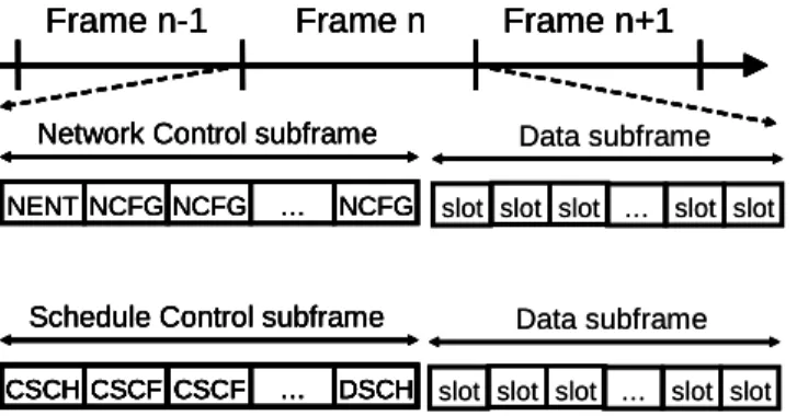
IEEE 802.16 mesh network is time-slotted. That is, the time is divided into equal-length time frames. And each time frame comprises one Control subframe and one Data subframe. Control subframe carries the control messages for the
Routing and Admission Control in IEEE 802.16
Distributed Mesh Networks
Tzu-Chieh Tsai and Chuan-Yin Wang
Department of Computer Science, National Chengchi University, Taipei, Taiwan
[email protected], [email protected]
A
Token rate r Packet Queue Bucket size b Output Token rate r Packet Queue Bucket size b Output2
scheduling, entry of new stations, exchanging of basic network parameters, etc. The data frame is composed by the time-slots for the actual data transmissions. The frame structure is given in figure 2.
There are two kinds of control subframe: Network Control subframes and Schedule Control subframes. In Network Control subframes, MSH-NENT (Mesh-Network Entry) messages are used to provide the entries of new-coming stations. MSH-NCFG (Mesh-Network Configure) messages are sent by each station periodically to exchange the basic parameters of networks, such as: the identifier of the BS, hops to the BS, and neighbor number of the reporting stations…etc.
Two scheduling modes are defined in IEEE 802.16 mesh mode: centralized and distributed modes. In centralized scheduling mode, the BS is in charge of all the transmissions happening in the mesh network. The resources are allocated by the BS with the MSH-CSCH (Mesh-Centralized Scheduling) messages and MSH-CSCF (Mesh-Centralize Scheduling and Configure) messages. In distributed mesh mode, the scheduling information is carried by MSH-DSCH (Mesh-Distributed Scheduling) messages, whose transmission time is determined by the mesh election algorithm given in the standard. MSH-DSCH has four information elements (IEs): scheduling IE, request IE, availability IE, and grant IE. The Scheduling IE carries the information of next-transmission time used in the mesh election algorithm. The other three IEs are employed in the three-way handshake:
1. The MSH-DSCH:request is made along with MSH-DSCH:availability, which is used to indicates the potential timeslots of the source station.
2. MSH-DSCH:grant is sent in response indicating a subset of the suggested availabilities that fits, in possible, the request.
3. MSH-DSCH:grant is sent by the original requester containing a copy of the grant from the requester, to confirm the schedule.
After the three-way handshake indicated in figure 3, the reservation of timeslots in the data subframe is completed.
In both centralized and distributed mesh modes, the QoS can be supported by the fields of the CID (Connection Identifiers) that is associated with each connection. There are three fields that explicitly define the service parameters:
1. Priority: This field simply defines the service class of the connection
2. Reliability: To re-transmit or not.
3. Drop Precedence: The likelihood of dropping the packets when congestion occurs.
III. RELATED WORK
H. Shetiya and V. Sharma [2] proposed the algorithms of routing and scheduling under IEEE 802.16 centralized mesh networks. The routing metric is based on the evaluation of queue length on each station. The routing is fixed routing, which reduces the topology into a tree. The scheduling algorithm is based on a mathematical model to allocate enough timeslots among the traffic flows. And our previous work [3] that focus on the call admission control and packet scheduling in the IEEE 802.16 PMP mode. In this paper, a mathematical model is proposed to characterize the packets of different traffic flows.
Some other researches also focus on the IEEE 802.16 mesh mode: F. Liu et al. [4] proposed a slot allocation algorithm based on priority, which is to achieve QoS. Z. J. Haas et al. [5] proposed an approach to increase the utilization of IEEE 802.16 mesh mode. They have adopted a cross-layer design in their work. M. Cao et al. [6] proposed a mathematical model and an analysis of IEEE 802.16 mesh distributed scheduler, mostly on the mesh election algorithm.
Douglas, S, J. De Couto et al. [7] proposed a new routing metrics called “ETX”, short for “Expect Transmission Count”. ETX is suitable for wireless networks and is able to fit in any routing algorithms like DSR, DSDV … etc.
IV. ROUTING METRICS:SWEB
a new routing metrics called SWEB (Shortest-Widest Efficient Bandwidth) is proposed, which considers three parameters: packet error rate, Pi,j , capacity Ci,j over the link (i,j) and the hop count, h, from the source to the destination. The packet error rate can be retrieved by the exchanging of MSH-DSCH messages, which is associated with a unique sequence number. The lost or error MSH-DSCH messages can be detected. And the link capacity can be also known by the burst profile indicated in the MSH-NCFG messages. In MSH-NCFG messages, the hop count for a station to base station is also given. Therefore, we argue that our SWEB metrics is especially suitable for IEEE 802.16 mesh networks. The efficient bandwidth of a link (i,j) can be calculated as:
Frame n-1
Frame n
Frame n+1
NENT NCFG NCFG … NCFG
Network Control subframe
CSCH CSCF CSCF … DSCH
Schedule Control subframe
Frame n-1
Frame n
Frame n+1
NENT NCFG NCFG … NCFG
Network Control subframe
CSCH CSCF CSCF … DSCH CSCH CSCF CSCF … DSCH
Schedule Control subframe
Data subframe
slot slot slot … slot slot
Data subframe
slot slot slot … slot slot
Frame n-1
Frame n
Frame n+1
NENT NCFG NCFG … NCFG
Network Control subframe
CSCH CSCF CSCF … DSCH CSCH CSCF CSCF … DSCH
Schedule Control subframe
Frame n-1
Frame n
Frame n+1
NENT NCFG NCFG … NCFG
Network Control subframe
CSCH CSCF CSCF … DSCH CSCH CSCF CSCF … DSCH
Schedule Control subframe
Data subframe
slot slot slot … slot slot
Data subframe
slot slot slot … slot slot
Fig. 2. Frame structures of IEEE 802.16 mesh mode.
Requester Granter MSH-DSCH:Request And MSH-DSCH:availbility MSH-DSCH:Grant MSH-DSCH:Grant Requester Granter MSH-DSCH:Request And MSH-DSCH:availbility MSH-DSCH:Grant MSH-DSCH:Grant
3 ) 1 ( . ,j ij i p C − (1) However, since the flow that comes in and leaves a node shares the bandwidth. Equation (1) should be divided by two to represent the available bandwidth. Therefore, the end-to-end available bandwidth is:
2 )) 1 ( ),..., 1 ( ), 1 ( min(C1,2⋅ −p1,2 C2,3⋅ −p2,3 Ci,j⋅ −pi,j (2) By using (2), we define our SWEB metrics for all potential paths as: h p C p C p C SWEB ij ij 1 2 )) 1 ( ),..., 1 ( ), 1 ( min( 1,2⋅ − 1,2 2,3⋅ − 2,3 , ⋅ − , ⋅ = (3) The path with the largest path metric will be chosen.
V. ADMISSION CONTROL ALGORITHM:TAC
Our Token bucket-based Admission Control (TAC) has two essential parts. First, the bandwidth used by a connection must be estimated well. Second, the bandwidth estimation is used for implementing the admission control algorithm.
A. Bandwidth Estimation
If all the connections are under the control of token bucket mechanism, the bandwidth used with a time frame can be estimated as:
f
b
f
r
i⋅
+
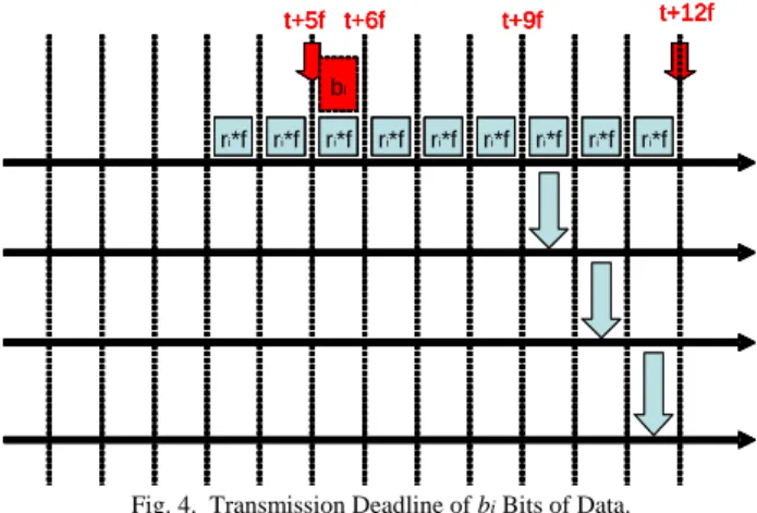
i (4) The ri and bi is the token rate and bucket size that associated with a connection i, respectively. f is the frame length. However, (3) is over-estimated since the transmission burst does not happen in every time frame. To better estimate the bandwidth, consider the scenario in figure 4.Let the hop count and transmission deadline of the flow in Fig. 6 is 3 and 7f, respectively. Assume that the transmission burst occurs in time interval [t+5f, t+6f] and tokens stored in the
bucket are completely consumed. In order to satisfy the delay requirement, these bi bits of data must be sent in [t+9f, t+10f] at latest. Therefore, the frames from t+6f to t+10f can be used for sharing the bi bits, as in figure 5.
Generally speaking, in order to meet the delay requirement, di, of real-time traffics, packets generated at time t
have to be sent after mi frames after t, where
h f d m i i ⎥− ⎦ ⎥ ⎢ ⎣ ⎢ = (4) These mi frames can be used to share the bi bits of data.
Therefore, the maximum volume of data that can be sent in any given frame is:
i i i
m
b
f
r
⋅
+
(5) We use (5) as bandwidth estimation of a flow.B. Admission Control
We use the above-mentioned bandwidth estimation to implement the TAC algorithm. In TAC algorithm, the minimum usage of timeslots by each connection is defined. They are: CBR_min, VBR_min and BE_min. When a station receives a MSH_DSCH:Request, it examines whether the current usage of each class exceeds their minimum usage or not. If it is, the new-coming flow will be marked as downgradedٛ flows. If a MSH-DSCH:Request comes in, the downgradedٛ flows have bigger possibilities to be preempted. On the other
t+6f ri*f ri*f ri*f ri*f t+12f t+5f ri*f ri*f ri*f ri*f ri*f t+9f bi/ mi-1 bi/ mi-1 t+6f ri*f ri*f ri*f ri*f t+12f t+5f ri*f ri*f ri*f ri*f ri*f t+9f t+6f ri*f ri*f ri*f ri*f t+12f t+5f ri*f ri*f ri*f ri*f ri*f t+9f bi/ mi-1 bi/ mi-1 t+6f ri*f ri*f ri*f ri*f t+12f t+5f ri*f ri*f ri*f ri*f ri*f t+9f
Fig. 5. Sharing bi Bits of Data.
t+6f ri*f ri*f ri*f ri*f t+12f t+5f bi ri*f ri*f ri*f ri*f ri*f t+9f t+6f ri*f ri*f ri*f ri*f t+12f t+5f bi ri*f ri*f ri*f ri*f ri*f t+9f t+6f ri*f ri*f ri*f ri*f t+12f t+5f bi ri*f ri*f ri*f ri*f ri*f t+9f t+6f ri*f ri*f ri*f ri*f t+12f t+5f bi ri*f ri*f ri*f ri*f ri*f t+9f
Fig. 4. Transmission Deadline of bi Bits of Data.
TABLEI QOSMAPPINGS 3 1 2 BE_DG 0 1 5 BE 2 0 3 VBR_DG 0 0 6 VBR 1 0 4 CBR_DG 0 0 7 CBR Drop Precedence (2 bits) Reliability (1 bit) Priority (3 bits) 3 1 2 BE_DG 0 1 5 BE 2 0 3 VBR_DG 0 0 6 VBR 1 0 4 CBR_DG 0 0 7 CBR Drop Precedence (2 bits) Reliability (1 bit) Priority (3 bits)
4 hand, if the current usage does not exceed its minimum usage,
the flow will not be downgrade and have bigger change to preempt other downgraded flows.
Since the service levels in IEEE 802.16 mesh mode are identified in the fields of CID (Connection Identifiers), we have the QoS mapping in Table I. With the mappings in table I, the down-graded flows can be marked. And by this information, we develop our TAC algorithm as follows:
1.) A new flow with its BW_req (Bandwidth request) in the unit of data timeslots. And set BW_avail as the total empty slot number. (BW_avail stands for available bandwidth) 2.) The station that handles the request checks if the
BW_req<BW_avail or not. If yes, go to step 3. Or else, go
to step 4.
3.) The station determines to downgrade the flow or not, by comparing the current usage and the minimum usage of the traffic class.
4.) The station checks if the current usage exceeds the minimum usage of the traffic class. If yes, the flow shall be rejected. Or else, go to step 5.
5.) Check the timeslots used by downgraded flows in the order of BE_DG, VBR_DG, and CBR_DG. If there is no such timeslots, the request is rejected. Or else, set this timeslots empty, which means to preempt this timeslots. Updating the value of BW_avail. Go to step 2.
VI. SIMULATION RESULTS
The simulations are conducted in a 16-node topology, and the simulation area is a 4 km * 4 km square. The radio range is set as 1.5 km in radius. The frame length is chosen to be 8 ms.
In the simulations, QPSK is chosen to be the modulation method. The details of QPSK are given in table II.
The data rate of the CBR traffic is 64 kbps, with the 960-bit packet size in the packet interval of 15 ms. The VBR traffic is sending at the average speed of 400 kbps. The mean packet size is 16000 bits sending at the interval of 40 ms. The packet size of BE traffics is 8000 bits and is sent every frame (8 ms).
A. Routing
The proposed SWEB is compared with the ETX [7] and the shortest path. The performance and delay of VBR traffics are compared across all three different metrics. The performance is given in figure 6. And figure 7 shows the delay.
As shown in the figure 6 and 7, when number of flows is reaching 25, some VBR flows are preempted by CBR flows. By simulation results, we claim that SWEB is a compromise of
delay and throughput. But in figure 8, we can find that SWEB has best performance in jitter of real-time packets.
B. Admission Control
In TAC algorithm, the minimum usage of each traffic class must be set. In the simulations, the CBR_min, VBR_min and
BE_min are set as 10, 40 and 75 timeslots, respectively. Also,
the parameters of token bucket are shown in table III.
TABLEII
THE PARAMETERS OF QPSK
QPSK coding rate 3/4
OFDM symbols in a frame 676 OFDM symbols in a control subframe 16
OFDM symbols in a data subframe 660 OFDM symbols in a timeslot 4
Number of data timeslots 165 Capacity of a timeslot 144 bytes
Throughput 0 1000 2000 3000 4000 5000 6000 7000 8000 5 10 15 20 25 number of flows bps ETX Shortest SWEB
Fig. 6. Throughput of VBR flows.
Avg. Delay 0 10 20 30 40 50 60 70 5 10 15 20 25 number of flows ms ETX Shortest SWEB
Fig. 7. Delay of VBR flows.
TABLEIII
TOKEN BUCKET MECHANISM PARAMETERS
Token rate (bytes / frame) Bucket size (bytes) Delay requirements CBR 120 8 40 ms VBR 1500 500 80 ms BE 7500 250 -- Jitter 0 5 10 15 20 25 30 35 5 10 15 20 25 Number of flows ti m e ( m s) ETX shortest SWEB
5
We compare the throughput in figure 9 and figure 10. In figure 9, BE traffics suffers from preemption from higher priority traffic class, therefore, receiving low throughput when network is heavily-loaded. By applying the CAC algorithm in figure 10, the BE flows has the guaranteed throughput by setting the minimum usage. The preemption occurs only in down-graded flows.
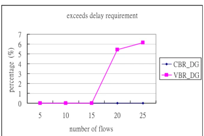
In figure 11 and figure 12, the statistics is gathered to discuss the percentage of real-time packets exceeds the delay requirements. As in figure 11, around 12% of VBR-packets exceed the delay requirements when the number of flow is 25. However, in figure 12 it is reduced to around 7% for only VBR-downgraded flows. It can be expected that for all VBR flows (VBR and VBR-downgraded), the ratio would be lower than 7%.
VII. CONCLUSIONS
In this paper, we proposed a new routing metric, SWEB, and an admission control algorithm, TAC for IEEE 802.16 mesh networks. SWEB is applied in static routing environment and yields the good throughput, delay and jitter performance. The TAC algorithm prevents the starvation of low-priority traffic flows and guarantees the delay requirements of the real-time flows. By SWEB and TAC, a QoS-enabled network environment can be realized with IEEE 802.16 mesh mode in the MAC layer. Thus, end-users will have better experience and convenience in utilizing the networks.
REFERENCES
[1] IEEE, “IEEE Standard for Local and metropolitan area networks Part 16: Air Interface for Fixed Broadband Wireless Access Systems”, IEEE standard, October 2004.
[2] Harish Shetiya and Vinod Sharma, "Algorithms for routing and centralized scheduling to provide QoS in IEEE 802.16 mesh networks",
Proceedings of the 1st ACM workshop on Wireless multimedia networking and performance modeling ,WMuNeP '05. Pages: 140-149.
[3] Tzu-Chieh Tsai, Chi-Hong Jiang, and Chuang-Yin Wang, "CAC and Packet Scheduling Using Token Bucket for IEEE 802.16 Networks", in Journal of Communications (JCM, ISSN 1796-2021), Volume : 1 Issue : 2, 2006. Page(s):30-37. Academy Publisher.
[4] Fuqiang LIU, Zhihui ZENG, Jian TAO, Qing LI, and Zhangxi LIN, "Achieving QoS for IEEE 802.16 in Mesh Mode",8th International
Conference on Computer Science and Informatics, Salt Lake City, USA
[5] Hung-Yu Wei, Samrat Ganguly, Rauf Izmailov, and Zygmunt J. Haas, "Interference-Aware IEEE 802.16 WiMax Mesh Networks", in
Proceedings of 61st IEEE Vehicular Technology Conference (VTC 2005
Spring).
[6] Min Cao, Qian Zhang, Xiaodong Wang, and Wenwu Zhu, "Modelling and Performance Analysis of the Distributed Scheduler in IEEE 802.16 Mesh Mode", Proceedings of the 6th ACM international symposium on Mobile
ad hoc networking and computing
[7] Douglas S. J. De Couto, Daniel Aguayo, John Bicket , and Robert Morris, “A High-Throughput Path Metric for Multi-Hop Wireless Routing”, ACM
MobiCom ’03.
exceeds delay requirement
0 2 4 6 8 10 12 14 5 10 15 20 25 number of flows pe rcen ta ge ( % ) CBR VBR
Fig. 11. The ratio of the realtime packets that exceeds the delay requirements for the original IEEE 802.16 mesh mode.
(TAC) throughput 0 1000 2000 3000 4000 5000 6000 7000 8000 5 10 15 20 25 number of flows bps CBR VBR BE total
Fig. 10. Throughput when TAC is applied.
throughput 0 1000 2000 3000 4000 5000 6000 7000 8000 5 10 15 20 25 number of flows bp s CBR VBR BE total
Fig. 9. Throughput for the original IEEE 802.16 mesh mode.
exceeds delay requirement
0 1 2 3 4 5 6 7 5 10 15 20 25 number of flows percent age (% ) CBR_DG VBR_DG
Fig. 12. The ratio of the realtime packets that exceeds the delay requirements when TAC is applied.
Modeling the Distributed Scheduler of IEEE 802.16 Mesh Mode
Tzu-Chieh Tsai, Yan-Bin Chen
Computer Science Department, National Chengchi University
Taipei, Taiwan, [email protected]
Taipei, Taiwan, [email protected]
Abstract
The IEEE 802.16 standard is a protocol for wireless metropolitan networks. IEEE 802.16 MAC protocol supports both of PMP (point to multipoint) and Mesh mode. In the mesh mode, all nodes are organized in a similar ad-hoc fashion and calculate their next transmission time based on the scheduling information performed in the control subframe. Each node has to compete with each other to win the time slots of opportunities for the subsequent advertisement of the scheduling messages to its neighbors. This behavior does not depend on all of past history. In other words, it is a “Time Homogeneous” and suitable for being modeled by stochastic process. In this study, we will model this scheduling behavior by queuing process, and apply the Markov Chain to estimate its average delay time which a node keep waiting until it win the competition.
1. I
NTRODUCTIONThe IEEE 802.16 standard [1, 2] “Air Interface for Fixed Broadband Wireless Access Systems”, also known as WiMAX, targets at providing last-mile wireless broadband access in metropolitan area networks. IEEE 802.16 is a wireless network, which has the high capacity to cover more broad geographic areas without the costly infrastructure development. The technology may prove less expensive to deploy and may lead to more ubiquitous broadband access [3]. The clients also can connect to the IEEE 802.16 by adopting various existing wireless solutions, such as IEEE 802.11 (WiFi). IEEE 802.16 provides a cheaper and more ubiquitous solution to connect home or business to Internet. Much attention was paid to the IEEE 802.16 issues in recent years and a lot of industries formed a WiMAX Forum in order to certify compatibility and interoperability of various 802.16 products.
The 802.16 mesh mode topology is depicted as Fig.1. There are many SSs in this topology which terminals, such as PDAs, notebooks or cellular phones, can be connected to via 802.11 or other protocols. The mesh mode is organized throughout these SSs and BSs. The link coverage is expanded under mesh network. Certain SSs are responsible to connect to the BSs. By these BSs, they connect to the backhaul or internet.
Besides, a Markov Chain to model this distributed scheduling of mesh mode as well as a mathematical model are proposed in this paper to evaluate the average delay time.
Fig. 1: IEEE 802.16 Mesh Mode Topology
2. A
NALYZEIEEE
802.16
D
ISTRIBUTEDS
CHEDULINGA
LGORITHMBefore we model the Distributed Scheduler in IEEE 802.16 mesh mode, we have to know its behavior.
A. 802.16 Mesh MAC Frame Structure
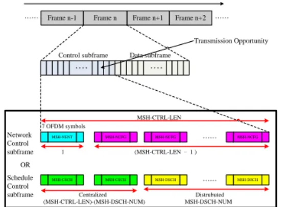
The IEEE 802.16 defined the mesh frame structure as a convenience to organize the mesh network. The frame is divided into two subframes. One is the data subframe, the other is control subframe. Every control subframe consists of sixteen transmission opportunities, which may be imaged as a “time slot”, and every transmission opportunity equals seven OFDM symbols time.
There are two control subframe types in a control subframe. One is network control subframe that creates and maintains the cohesion between different systems. It also provides a new node to gain synchronization and initial network entry into a mesh network. The other is a subframe that to coordinate scheduling of data transfers in system, called schedule control subframe. The scheduling information is encapsulated here. Frames with the network control subframe occur periodically and all the other frames contain schedule control subframes along the network control subframe.
Two messages NENT” and “MSH-NCFG” are used in the network control subframe. MSH-NENT means a mesh network entry, which is a message for a new node to gain synchronization and initial network entry into a mesh network; furthermore, MSH-NCFG means a mesh network configuration, provides a basic information of communication between nodes in different nearby networks. On the side, in the schedule control subframe, “MSH-CSCH” and “MSH-DSCH” means the mesh network centralized scheduling and the mesh network distributed scheduling, separately. MSH-DSCH is the key point that this paper will concentrate on.
We have introduced that every control subframe consists of sixteen transmission opportunities. Nevertheless, they are just the opportunities to own these time slots, but the really time slot occupied is indicated by “MSH-CTRL-LEN”. MSH-CTRL-LEN is a field saved in the MSH-NCFG message to express the control subframe length. MSH-DSCH-NUM is also saved in the MSH-NCFG message to express the number of MSH-DSCH opportunities in the schedule control subframe. Of course, what’s left after MSH-DSCH-NUM is subtracted from MSH-CTRL-LEN becomes the number of MSH-CSCH opportunities. All of the parameters we introduced thus far are depicted in Fig. 2. MSH-NENT MSH-NCFG MSH-NCFG MSH-NCFG 1 (MSH-CTRL-LEN – 1 ) MSH-CTRL-LEN MSH-CSCH MSH-CSCH MSH-DSCH MSH-DSCH Centralized Distrubuted MSH-DSCH-NUM (MSH-CTRL-LEN)-(MSH-DSCH-NUM) …… …… 7 OFDM symbols Frame n+1 Frame n+2 Frame n Frame n-1 Time …… ……
Control subframe Data subframe
Transmission Opportunity OR Network Control subframe Schedule Control subframe
Fig. 2: Network Control subframe and Schedule Control subframe
B. Next Transmission Time and Transmission Holdoff Time
In this section, we will introduce parts of the terminologies and abbreviations in the IEEE 802.16 specification.
The schedule information for each node is described by two parameters Next Xmt Time and Xmt holdoff Time. In the IEEE 802.16 specification, Next Xmt Time is not employed directly. It uses Next Xmt Mx to calculate the Next Xmt Time. It doesn’t use Xmt holdoff Time, neither. It uses Xmt holdoff exponent to calculate the Xmt holdoff Time. As the Fig. 3 shows, Next Xmt Mx and Xmt holdoff exponent are two parameters in the MSH-DSCH message to perform the schedule information. So that whenever a node transmits MSH-DSCH message, every node has the schedule information of its neighbors.
Fig. 3: Next Xmt Mx and Xmt holdoff exponent in the MSH-DSCH (source: IEEE 802.16-2004)
A node has to decide the next transmission time to know when to transmit the next MSH-DSCH message. There is a special terminology employed in the IEEE 802.16 specification to describe this transmission duration named “Eligible Interval”. This next transmission time is denoted as Next Xmt Time and calculated from Next Xmt Mx. Assume “Next” is denoted as Next Xmt Time of an observed node; “Mx” and “x” means its corresponding Next Xmt Mx and Xmt holdoff exponent separately. Duration of Next Xmt Time could be shown as the following formula (1) defined in the standard. By the observation of this formula, we know 2 is the length of “Next”. “x” is x clearly an exponential value to express the length of “Next”.
(1)
Xmt Holdoff Time is also a special terminology applied in the IEEE 802.16 specification to indicate that this node is not eligible to transmit messages. Assume “Holdoff” is denoted as Xmt Holdoff Time of an observed node; “x” means its corresponding Xmt holdoff exponent. Then, Xmt Holdoff Time could be shown as the following formula(2) defined in the standard. We know 2 is the length of “Next”. From x this formula, we know the holdoff time is in multiples of sixteen “Next”.
(2)
The following figure shows these variations on time axis. (Fig. 4) Earliest Subsequent Xmt Time is a terminology in the standard to denote the earliest possible transmission time, without been determined.
Fig. 4: Next Xmt Time and Xmt Holdoff Time
C. Competing Behavior and Scheduling Algorithm
Distributed scheduling ensures that the transmissions are collision-free. There is an election algorithm named MeshElection defined in the IEEE 802.16 standard to achieve collision-free.
The competing behavior and scheduling algorithm occur in each of nodes which are activating all over
NextXmtTime XmtHoldoffTime EarliestSubsequentXmtTime Eligible Interval XmtHoldoffTime 1) (Mx 2 Next Mx 2x⋅ < ≤ x⋅ + 4 x 2 Holdoff = +
the neighborhood in mesh network. For instance, we observe certain node’s competing behavior and its scheduling algorithm. We assume this node as an observed node; its neighboring nodes are denoted as neighbors. In the period of the competing behavior happened on this observed node, the scheduling algorithm is been computed. (3) is a formula to get the Earliest Subsequent Xmt Time over its all neighbors. Formula (4) sets Temp Xmt Time equal to this observed node’s Xmt Holdoff Time added to the current Xmt Time.
(3)
(4)
Depends on the information obtained previously, the observed node has the sufficient information to judge whether the possible collisions will occur or not. That is, there is a probability that this observed node’s Next Xmt Time results in collision with neighbors’ Next Xmt Time. The competing nodes are the subset of the neighbors with a Next Xmt Time eligibility interval that includes Temp Xmt Time or which an Earliest Subsequent Xmt Time equal to or smaller than Temp Xmt Time. These collision situations are depicted as Fig. 5 to express the collisions will be occurred between an observed node’s Next Xmt Time and its neighbors’. The neighbor i is save. The neighbor j has its Next Xmt Time at the same time with the observed node. Neighbor k owns its Next Xmt Time early but its Earliest Subsequent Xmt Time overlaps the observed node’s Next Xmt Time. In brief, observed node has two collisions with neighbor j and neighbor k.
NextXmtTime XmtHoldoffTime Observed node Nbr. j Nbr. i
Nbr. k Earliest Subsequent Xmt Time
Fig. 5: One node results in collision with neighbors
If the collision will happen on observed node’s Next Xmt Time as mentioned previously, the algorithm MeshElection will be executed during this computing period of distributed schedule. MeshElection is a C code function implemented in the standard. The Boolean value will be come out after MeshElection. “TRUE” means that this observed node wins the competing; on the contrary, “FALSE” means not. Corresponding procedures of them are:
TRUE: Set Temp Xmt Time to Next Xmt Time, and ends off this algorithm.
FALSE: Temp Xmt Time need to back.
D. Three-Way Handshaking
Thansmiting the MSH-DSCH message to the neighbors shall stable then subsequent data transmission may work better. Before data transmission, both of the coordinated and uncoordinated scheduling employs a three-way handshake to setup the connections with neighbors. This mechanism is used to convey the channel resources for the preparation of consequent data transmission. As follows, the three-way handshaking IEs (information elements) “Request IE”, “Availability IE” and “Grants IE” are encapsulated in the MSH-DSCH. Hence it implies that the performance of MSH-DSCH packet traffic influences the three-way handshaking. This is why we concentrate upon the MSH-DSCH performance evaluation in this paper.
3.
M
ATHEMATICM
ODELSo far, the competing behaviors of control subframe in the distributed scheduling of IEEE 802.16 mesh mode are presented. Next, we are going to propose a mathematical analysis to model the MSH-DSCH transmission behavior of IEEE 802.16 mesh mode. The delay time of MSH-DSCH transmission will be evaluated by our proposed mathematical model.
Assume X is denoted as a state in our n
consequent Markov Chain model that a node stays at a certain time to transmit MSH-DSCH. Time unit is an opportunity. A set of random variable {Xn}forms a Markov chain if the probability that the next state is
1 n+
X
depends only upon the current stateX
n andnot upon any previous stations. Base on our analysis in previous section, the next state merely depends on the current competing result, neither on the last nor on all of past history. Thus we have a random sequence in which the dependency extends backwards one unit in time. If this node’s Temp Xmt Time overlaps with its neighbors, it implies the competing is occurred with them. If it wins or there is no competition, it will set this Temp Xmt Time as its Next Xmt Time. If it loses, it will back one opportunity to run this behavior again until it wins. In order to simplify the notification, we assume integer 1,2,3 … represent each of certain state
n
X
, the physical concept of our proposed MarkovChain are depicted as Fig.6.
Next Xmt Time Xmt Holdoff Time Time Current Xmt Time 1 2 x 2 Fig. 6: Each state corresponds to the Next Xmt Time
With this concept of Fig.6, we can model this behavior with a vertical chain as Fig.7. The states and transition definitions are defined as Table 1. From Time Holdoff Xtm Time Xmt Next Time Xtm Subsequent Earliest + = Time Holdoff Xtm Time Xmt Current Time Xtm Temp = +
state 1 to state
2
x implies the time duration of one Next Xmt Time. Suppose we have N nodes totaly, the probability which a node wins N-1 nodes can be gotten by expression (5). Oppositely, the probability of a node loses them can be gotten by equation (6).(5) (6)
TABLE 1:THE NOTATION DEFINITIONS IN THE MARKOV
CHAIN
Notation Description Integers in
the state
The state probability that the transmission time backs to certain opportunity
Prob The transition probability to indicate the probability that the node wins.
x Exponent of Xmt Holdoff Time N The number of nodes
For example, if our observed node loses, it transfers from state 1 to state 2, the transition probability is 1-ProbN-1. If it wins, it stays at state 1,
the transition probability is
Prob
N-1.1 2 ProbN-2 1 ProbN-1 1-ProbN-1 x 2 Fig. 7: One vertical chain
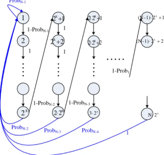
In order to model it easily, we assume that as long as the node lose this competition, it does not back one opportunity. It has to back a length of Next Xmt Time. That’s why the transition probabilities during the inter-states are always 1 in Fig.7. At last, a Markov chain is organized as Fig8
1 2 1-ProbN-2 ProbN-2 1 1 1 1-ProbN-3 ProbN-3 ProbN-4 ProbN-1 1-ProbN-1 x 2 2⋅ x 2 x 2 3⋅ 1 2x+ 2 2x+ 1 2 2⋅x+ 2 2 2⋅x+ 1 x 2 N⋅ 1 2 1) -(N ⋅ x+ 2 2 1) -(N ⋅ x+ 1-Prob1
Fig. 8: The Markov Chain
The Markov Chain we proposed presents the variation of state transitions. We hope to induce an equation to evaluate the average delay time. The dependency of delay time relates to a probability of win. Before evaluating the delay time, we have to induce this probability formula initially. Then the expected value which is just the average delay time we target is the product of probability and time.
To begin with, we assume the number of nodes is N. Each observation of a node competes with neighbors is independent and represents one of two outcomes "competing" or "non-competing". So formula (7) is obtained and it is the extension of binomial distribution we know. The
P
c in the (7) is a probability that a node competes with one another node.P
competing is different fromP
c in ourassumptions.
P
c is the condition happened betweenone node and one node in a very short time. Nevertheless,
P
competing is the condition while at least one of the following events is happened: between one node and one node, or between one node and two nodes, or between one node and more another nodes. So formula (7) means one of the following situations is occurred: observed node competes with one neighbor and wins, or observed node competes with two neighbors and wins, or observed node competes with three neighbors and wins …etc.TABLE 2:
N
OTATIONS OF EQUATIONSNotation Description
Prob Probability of
(
competing
∩
win
)competing
P
Probability of competing, at least one of more events happens1 -N Prob Win= 1 -N
Prob
-1
Lose
=
c
P
Probability of competing between one node to one of another node. N Number of nodes(7)
In opposition, the losing probability can be derived as (8).
(8)
If the node wins at state 1, the transition probability of win can be expressed by using (9). If the node wins at the state
2
xthat is the end of first vertical chain, the probability of win can be expressed by using (10).(9)
(10)
This probability distribution gives the trial number of the first success, so it is a geometric distribution. Substitute (7) and (8) into (9) and (10), we can derive the probability (11) and (12).
(11)
(12)
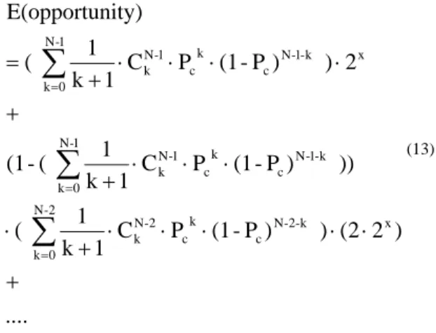
So far, each probability on the corresponding vertical chain has been derived. The expected value can be calculated by the summation of these probabilities and multiplied by time. Then fomular (13) can be obtained. The unit of time in this formula is opportunity.
....
)
2
2
(
)
)
P
-(1
P
C
1
k
1
(
))
)
P
-(1
P
C
1
k
1
(
-(1
2
)
)
P
-(1
P
C
1
k
1
(
ity)
E(opportun
x k -2 -N c k c 2 -N k 2 -N 0 k k -1 -N c k c 1 -N k 1 -N 0 k x k -1 -N c k c 1 -N k 1 -N 0 k+
⋅
⋅
⋅
⋅
⋅
+
⋅
⋅
⋅
⋅
+
+
⋅
⋅
⋅
⋅
+
=
∑
∑
∑
= = = (13)Finally, we generalize our equation, as (14). In conclusion, the input parameters are N and x. It means the delay time is affected by the number of nodes and holdoff exponent.
(14)
4.
S
IMULATIONR
ESULTWe validate our model is this section. The transmission behavior is simulated by our C code. The mathematic evaluations are computed by the MATLAB 7.0. Following parameters are applied: Exponent = 2
Node ID: random number between 1~4095 Probability: Pc= 0.5
And the result is shown as Fig.9. With this figure, it shows our mathematical model approaches the simulation result.
2~20 Nodes 0 20 40 60 80 100 120 2 4 6 8 10 12 14 16 18 20 Number of nodes opp or tunitie s( tim e sl ot ) sim math p=0.5
Fig. 9: The delay time of opportunities between simulation and mathematic model
The error rate is shown as Fig.10. It shows the error is under 10% while the nodes of number between 2 to 20.
k -1 -N c k c 1 -N k 1 -N 0 k 1 -1 -N c 1 c 1 -N 1 1 -N c 0 c 1 -N 0 win competing 1 -N ) P -(1 P C 1 k 1 ... ) P -(1 P C 2 1 ) P -(1 P C 1 1 P Prob ⋅ ⋅ ⋅ + = + ⋅ ⋅ + ⋅ ⋅ = =
∑
= ∩ ) ) P -(1 P C 1 k 1 ( -1 Prob -1 N-1-k c k c 1 -N k 1 -N 0 k 1 -N =∑
+ ⋅ ⋅ ⋅ = 1 -NProb
2 -N 1 -N ) Prob Prob -(1 ⋅)
)
P
-(1
P
C
1
k
1
(
Prob
k -1 -N c k c 1 -N k 1 -N 0 k 1 -N⋅
⋅
⋅
+
=
∑
=)
)
P
-(1
P
C
1
k
1
(
))
)
P
-(1
P
C
1
k
1
(
-(1
Prob
)
Prob
-(1
k -2 -N c k c 2 -N k 2 -N 0 k k -1 -N c k c 1 -N k 1 -N 0 k 2 -N 1 -N⋅
⋅
⋅
+
⋅
⋅
⋅
⋅
+
=
⋅
∑
∑
= = j) )(2 ) P -(1 P C 1 k 1 .( )) ) P -(1 P C 1 k 1 ( -(1 ity] E[opportun x k -i -N c i -N 0 k k c i -N k N 2 j 1 -j 1 i k -1) -(i -N c 1) -(i -N 0 k k c 1) -(i -N k ⋅ + + =∑
∑∏
∑
= = = =2~20 Node Error Rate 0 10 20 30 40 50 60 70 80 90 100 2 4 6 8 10 12 14 16 18 20 Number of nodes E rro r ra te ( 10 0% ) Error rate(%)
Fig. 10: The error rate between simulation and mathematic model
5.
C
ONCLUSIONS AND FUTURE WORKSIn this paper, we have presented a Markov chain model which can be used to simulate real MSH-DSCH transmission behavior in 802.16 mesh mode. This model considers the competing probability and back behavior of MSH-DSCH. Base on this model, we derive a formula to evaluate an average delay time of MSH-DSCH transmission.
R
EFERENCES[1] IEEE, “802.16 IEEE Standard for Local and metropolitan area networks, Part16:Air Interface for Fixed Broadband Wireless Access Systems”, IEEE Std 802.16dTM 2004, 1 October 2004. [2] IEEE, “802.16 IEEE Standard for Local and
metropolitan area networks, Part16:Air Interface for Fixed and Mobile Broadband Wireless Access Systems, Amendment 2: Physical and Medium Access Control Layers for Combined Fixed and Mobile Operation in Licensed Bands and Corrigendum 1”, IEEE Std 802.16eTM 2005, 28 February 2005.
[3] Carl EKlund, Roger B. Marks, Kenneth L. Stanwood, and Stanley Wang, “IEEE standard 802.16: A technical overview of the wirelessMAN air interface for broadband wireless access”, IEEE Communications Magazine, vol. 40, no. 6, June 2002, pp. 98-107.
[4] Arunabha Ghosh, David R. Wolter, Jeffrey G. Andrews, and Runhua Chen, “Broadband Wireless Access with WiMax/8O2.16: Current Performance Benchmarks and Future Potential”,
IEEE Communications Magazine, pages 129–136, February 2005.
[5] Dave Beyer, Nico van Waes, Carl EKlund, “Tutorial: 802.16 MAC Layer Mesh Extensions Overview”,
http://www.ieee802.org/16/tga/contrib/S80216a-02_30.pdf, 2002
[6] Nico Bayer, Dmitry Sivchenko, Bangnan Xu, Veselin Rakocevic, Joachim Habermann, “Transmission timing of signaling messages in IEEE 802.16 based Mesh Networks”, European Wireless 2006, Athens, Greece, April 2006. [7] Fuqiang LIU, Zhihui ZENG, Jian TAO, Qing LI,
and Zhangxi LIN, “Achieving QoS for IEEE 802.16 in Mesh Mode”, 8th International Conference on Computer Science and Informatics, Salt Lake City, USA.
[8] Simone Redana, Matthias Lott “Performance Analysis of IEEE 802.16a in Mesh Operation Mode”, Lyon, France, June 2004.
[9] Min Cao, Wenchao Ma, Qian Zhang, Xiaodong Wang, Wenwu Zhu, “Modelling and Performance Analysis of the Distributed Scheduler in IEEE 802.16 Mesh Mode”, In MobiHoc ’05: Proceedings of the 6th ACM international symposium on Mobile ad hoc networking and computing, pages78–89, NewYork, NY, USA, ACM Press, May 2005.
[10] Hung-Yu Wei, Samart Ganguly, Rauf Izmailov, and Zygmunt J. Haas, “Interference-Aware IEEE 802.16 Wimax Mesh Networks”, volume5, pages3102–3106, 2005.
[11] Leonard Kleinrock, “QUEUEING SYSTEMS VOLUME I: THEORY”, p26, 1976.
[12] Harish Shetiya, Vinod Sharma, “Algorithms for Routing and Centralized Scheduling to Provide QoS in IEEE 802.16 Mesh Networks”, ACM, October 2005.
[13] Tzu-Chieh Tsai, Chi-Hong Jiang, and Chuang-Yin Wang, “CAC and Packet Scheduling Using Token Bucket for IEEE 802.16 Networks”, in Journal of Communications (JCM, ISSN 1796-2021), Volume : 1 Issue : 2, 2006. Page(s): 30-37. Academy Publisher.