利用精神分裂症資料來比較五種常用的偵測基因基因交互作用效果的方法

國 立 交 通 大 學

統計學研究所

碩 士 論 文

利用精神分裂症資料來比較五種常用的偵測

基因基因交互作用效果的方法

Comparison of Five Commonly Used Gene-Gene

Interaction Detecting Methods in Schizophrenia

研 究 生：謝重耕

指導教授：黃冠華 博士

利用精神分裂症資料來比較五種常用的偵測

基因基因交互作用效果的方法

Comparison of Five Commonly Used Gene-Gene

Interaction Detecting Methods in Schizophrenia

研 究 生：謝重耕 Student: Chung-Keng Hsieh

指導教授：黃冠華 Advisor: Dr. Guan-Hua Huang

國 立 交 通 大 學

統計學研究所

碩 士 論 文

A Thesis

Submitted to institute of Statistics College of Science

National Chiao Tung University in Partial Fulfillment of the Requirements

for the Degree of Master

in Statistics June 2008

Hsinchu, Taiwan, Republic of China

Comparison of Five Commonly Used Gene-Gene

Interaction Detecting Methods in Schizophrenia

Student: Chung-Keng Hsieh Advisor: Dr. Guan-Hua Huang

Institute of Statistics

National Chiao Tung University

ABSTRACT

There are more evidences that gene-gene interaction is probably ubiquitous in complex disease. Several statistical methods have been developed to detecting such association. We are interesting in how to use these methods in a real data and want to compare these methods. In the present study, we applied five commonly used methods: chi-square test, logistic regression model (LRM), bayesian epistasis association mapping (BEAM) algorithm, classification and regression trees (CART), and the multifactor dimensionality reduction (MDR) method to a schizophrenia case-control dataset. Our study show evidence for several single marker effects and gene-gene interactions associated with schizophrenia. At the final part, in order to assess the ability of prediction with these five methods, cross-validation is also proposed along with these methods.

利用精神分裂症資料來比較五種常用的偵測

基因基因交互作用效果的方法

研究生：謝重耕 指導教授：黃冠華 博士

國立交通大學統計學研究所

摘要

有越來越多的證據顯示，基因基因交互作用是普遍存在於常見複雜性疾病之 中的。為了發現這些交互作用與疾病的相關性，已經發展出了許多的統計方法。 我們有興趣的是如何使用這些方法來實際分析資料，並且想要比較這些方法。在 這個研究中，我們利用五種常用的方法：卡方檢定、邏輯迴歸模型（LRM）、 bayesian epistasis association mapping (BEAM) algorithm 、 classification and regression trees (CART) 以及 the multifactor dimensionality reduction (MDR) method 來分析一組精神分裂症的病例－對照研究資料。我們的分析顯示，有一

些顯著的單一 marker 效果以及基因基因交互作用效果是與精神分裂症有高度相

關的。在研究的最後部份，我們希望能比較這五種方法在預測疾病狀態上的能

力，我們利用cross-validation 來比較這五種方法的預測能力。

誌 謝

兩年的研究生生活，想不到轉眼間就到了最後的階段，要畢業了。首先要感 謝的人，自然是我的指導教授，黃冠華老師。在做研究的這段時間，常常去詢問 老師許多問題，meeting時與老師討論的過程中也給了我許多的建議。老師的幫 助是這篇論文能順利完成的最大推手。另外，也要感謝當我到中研院學習時，楊 欣洲老師、花文妤學姐的耐心指導，讓我能順利的踏入這個研究領域。還有跟我 一同打拼到最後的夥伴們，仲竹、小良、彥銘、佩芳。以及平時一起打球，一起 努力、一起度過這兩年的好朋友們，文廷、泰佐、翁賢、瑜達、政言和所有研究 室的好同學們。 同時，也感謝口試委員－陳君厚老師、楊欣洲老師及盧鴻興老師，對於這篇 論文給予了許多的建議。 還要感謝所有我的朋友、學長姐、以及所上老師們。對於我的學業、生活， 都給了我許多的幫助。 最後，要感謝我的父母及家人，還有阿關。是你們在我的背後默默的支持著 我，我才有力量能繼續的往前邁進。衷心感謝所有關心我、幫助我的人。 謝重耕 07.02.2008

Contents

ABSTRACT...i

摘要...ii

誌謝... iii

Tables and Figures Content ...v

1 INTRODUCTION...1 2 LITERATURE REVIEW...3 2.1 SNP...3 2.2 Genotype...4 2.3 Haplotype...4 2.4 Hardy-Weinberg equilibrium...6

2.5 Analytical approaches to interactions...8

2.5.1 Bayesian epistasis association mapping (BEAM)... 8

2.5.2 Classification and regression trees (CART) ... 13

2.5.3 Multifactor dimension reduction (MDR)... 15

3 MATERIALS AND METHODS...18

3.1 Study population...18

3.2 Preliminary analyses...18

3.3 Study design...20

3.4 Gene-gene interaction detecting methods...20

3.5 Cross-Validation (CV)...26

4 RESULTS ...28

5 CONCLUSION...32

Tables and Figures Content

Table 1. Marker’s Information...33

Table 2. Single marker effects detected by the five methods ...35

Table 3. Two-way interaction detected by the five methods ...36

Table 4. Three-way interaction detected by the five methods ...37

Table 5. Summary of rsDAO_13...39

Table 6. Summary of rsDAO_7...39

Table 7. Summary of DAO_block1 ...39

Table 8. Summary of rsDAO_6*rsDAO_7 ...41

Table 9. Average prediction error across 100 CVs ...42

Figure 1. Example of posterior probabilities of association for each marker by applying BEAM to our genotype-based data ...23

Figure 2. Example of applying CART to genotype-based data...25

Figure 3. Haplotype block...43

Figure 4. Box-plot of prediction error of one-way interaction ...45

Figure 5. Box-plot of prediction error of two-way interaction...46

1 INTRODUCTION

A grand challenge in statistical genetics is to develop powerful methods that can identify genes that control biological pathways leading to disease. Discovery of such genes is critical in the detection and treatment of human diseases. The dramatic advances in human genome research coupled with the recent progress in high-throughput technology for molecular biology and genetics now allow the study of the genetic basis of disease and the response to treatment of complex diseases, such as breast cancer, on a molecular level. A good example is the recent efforts of the Human Genome Project towards large-scale characterization of human single nucleotide polymorphisms (SNPs) [1].

Single-locus methods measure the effect of one locus irrespective of other loci and are useful to study genetic diseases caused by a single gene, or even loci within single genes. To study complex diseases such as cardiovascular disorders or diabetes single-locus methods may not be appropriate, as it is possible that loci contribute to a certain complex disease only by their interaction with other genes (epistasis), while main effects of the individual loci may be small or absent [2].

There is growing evidence that gene-gene interactions are ubiquitous in determining the susceptibility to common human diseases. The investigation of such gene-gene interactions presents new statistical challenges for studies with relatively small sample sizes as the number of potential interactions in the genome can be large [1]. Many have collected data on large numbers of genetic markers but are not familiar with available methods to assess their association with complex diseases. Statistical methods have been developed for analyzing the relation between large numbers of genetic and environmental predictors to disease or disease-related variables in genetic association studies [2].

Family, twin, and adoption studies have unequivocally demonstrated that genetic vulnerability is a major contributing factor in the etiology of schizophrenia. Although the details of schizophrenia’s pathophysiology remain to be worked out, current evidence indicates that it is a complex disorder influenced by genes, environmental risk factors, and their interaction [3-4].

In the present study, we assessed the importance of gene-gene interactions on schizophrenia risk by investigating 65 SNPs from 5 candidate genes in a sample of 514 cases and 376 controls. We discuss the methodological issues associated with the detection of gene-gene interactions in this dataset by applying and comparing five commonly used methods: the chi-square test, logistic regression model (LRM), bayesian epistasis association mapping (BEAM) algorithm, classification and regression trees (CART), and the multifactor dimensionality reduction (MDR) method. At the final part, in order to assess the ability of prediction with these five methods, cross-validation is also proposed along with these methods.

2 LITERATURE

REVIEW

2.1 SNP

(http://en.wikipedia.org/wiki/Single_nucleotide_polymorphism) A single nucleotide polymorphism (SNP, pronounced snip), is a DNA sequence variation occurring when a single nucleotide - A, T, C, or G - in the genome (or other shared sequence) differs between members of a species (or between paired chromosomes in an individual). For example, two sequenced DNA fragments from different individuals, AAGCCTA to AAGCTTA, contain a difference in a single

nucleotide. In this case we say that there are two alleles: C and T. In classical genetics the two alleles are usually denoted A and a. Almost all common SNPs have only two alleles. For a variation to be considered a SNP, it must occur in at least 1% of the population.

Within a population, SNPs can be assigned a minor allele frequency- the lowest allele frequency at a locus that is observed in a particular population. This is simply the lesser of the two allele frequencies for single nucleotide polymorphisms. It is important to note that there are variations between human populations, so a SNP allele that is common in one geographical or ethnic group may be much rarer in another. In the past, single nucleotide polymorphisms with a minor allele frequency of less than or equal to 1% (or 0.5%, etc.) were given the title "SNP," an unwieldy definition. With the advent of modern bioinformatics and a better understanding of evolution, this definition is no longer necessary.

Single nucleotide polymorphisms may fall within coding sequences of genes, non-coding regions of genes, or in the intergenic regions between genes. SNPs within a coding sequence will not necessarily change the amino acid sequence of the protein that is produced, due to degeneracy of the genetic code. A SNP in which both forms lead to the same polypeptide sequence is termed synonymous (sometimes called a

silent mutation) - if a different polypeptide sequence is produced they are non-synonymous. SNPs that are not in protein-coding regions may still have consequences for gene splicing, transcription factor binding, or the sequence of non-coding RNA.

Variations in the DNA sequences of humans can affect how humans develop diseases and respond to pathogens, chemicals, drugs, vaccines, and other agents. However, their greatest importance in biomedical research is for comparing regions of the genome between cohorts (such as with matched cohorts with and without a disease).

2.2 Genotype

(http://en.wikipedia.org/wiki/Genotype)

The genotype is the genetic constitution of a cell, an organism, or an individual, that is the specific allele makeup of the individual, usually with reference to a specific character under consideration. For instance, the human albino gene has two allelic forms, dominant A and recessive a, and there are three possible genotypes- AA (homozygous dominant), Aa (heterozygous), and aa (homozygous recessive).

A more technical example to illustrate genotype is the single nucleotide polymorphism or SNP. Returning to the SNP example with a C T substitution corresponding to A and a alleles, three genotypes are possible: AA, Aa and aa. Other types of genetic marker, such as microsatellites, can have more than two alleles, and thus many different genotypes. It is important that the two genotypes Aa and aA cannot be distinguished from each other, so the order of alleles does not matter [5].

→

2.3 Haplotype

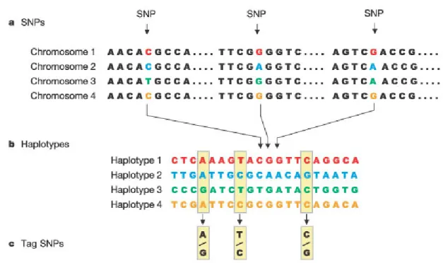
(http://en.wikipedia.org/wiki/Haplotype)

The term haplotype is a contraction of the term "haploid genotype." In genetics, a haplotype (Greek haploos = single) is a combination of alleles at multiple linked loci

that are transmitted together on the same chromosome. Haplotype may refer to as few as two loci or to an entire chromosome depending on the number of recombination events that have occurred between a given set of loci.

In a second meaning, haplotype is a set of single nucleotide polymorphisms (SNPs) on a single chromatid that are statistically associated. It is thought that these associations, and the identification of a few alleles of a haplotype block, can unambiguously identify all other polymorphic sites in its region. Such information is very valuable for investigating the genetics behind common diseases, and is collected by the International HapMap Project.

Figure : The construction of the HapMap occurs in three steps. (a) Single nucleotide polymorphisms (SNPs) are identified in DNA samples from multiple individuals. (b) Adjacent SNPs that are inherited together are compiled into "haplotypes." (c) "Tag" SNPs within haplotypes are identified that uniquely identify those haplotypes. By genotyping the three tag SNPs shown in this figure, researchers can identify which of the four haplotypes shown here are present in each individual.

Direct, laboratory-based haplotyping or typing further family members to infer the unknown phase are expensive ways to obtain haplotypes. Fortunately, there are statistical methods for inferring haplotypes and population haplotype frequencies from the genotypes of unrelated individuals. These methods, and the software that implements them, rely on the fact that in regions of low recombination relatively few of the possible haplotypes will actually be observed in any population. These programs generally perform well, given high SNP density and not too much missing data. SNPHAP is simple and fast, whereas PHASE tends to be more accurate but comes at greater computational cost. Recently FASTPHASE has emerged, which is nearly as accurate as PHASE and much faster [6].

2.4 Hardy-Weinberg equilibrium

(http://en.wikipedia.org/wiki/Hardy-Weinberg_principle)

In population genetics, the Hardy-Weinberg principle states that the genotype frequencies in a population remain constant or are in equilibrium from generation to generation unless specific disturbing influences are introduced. Those disturbing influences include non-random mating, mutations, natural selection, limited population size, random genetic drift and gene flow. Genetic equilibrium is a basic principle of population genetics. This concept is also known by a variety of names: HWP, Hardy–Weinberg equilibrium, HWE, or Hardy–Weinberg law. It was named after G. H. Hardy and Wilhelm Weinberg.

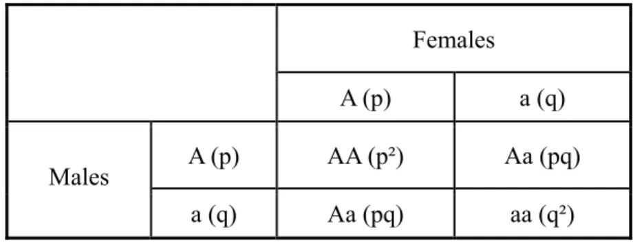
A better, but equivalent, probabilistic description for the HWP is that the alleles for the next generation for any given individual are chosen randomly and independent of each other. Consider two alleles, A and a, with frequencies p and q, respectively, in the population. The different ways to form new genotypes can be derived using a Punnett square (also known as a Prout Square), where the fraction in each is equal to

the product of the row and column probabilities.

Table : Punnett square for Hardy–Weinberg equilibrium

Females

A (p) a (q)

A (p) AA (p²) Aa (pq)

Males

a (q) Aa (pq) aa (q²)

The final three possible genotypic frequencies in the offspring become:

„ _{( )} 2

f AA = p „ f Aa( ) 2= pq

„ _{( )} 2

f aa = q

These frequencies are called Hardy-Weinberg frequencies (or Hardy-Weinberg proportions). This is achieved in one generation, and only requires the assumption of random mating with an infinite population size. Sometimes, a population is created by bringing together males and females with different allele frequencies. In this case, the assumption of a single population is violated until after the first generation, so the first generation will not have Hardy-Weinberg equilibrium. Successive generations will have Hardy-Weinberg equilibrium.

Testing for deviations from HWE can be carried out using a Pearson goodness-of-fit test, often known simply as “the _χ2 _{test” because the test statistic} has approximately a _χ2 _{null distribution. Be aware, however, that there are many} different _χ2 _{tests. The Pearson test is easy to compute, but the χ}2 _{approximation} can be poor when there are low genotype counts, and it is better to use a Fisher exact test, which does not rely on the _χ2 _{approximation. The open-source data-analysis}

software R has an R genetics package that implements both Pearson and Fisher tests

of HWE, and PEDSTATS also implements exact tests [6].

2.5 Analytical approaches to interactions

2.5.1 Bayesian epistasis association mapping (BEAM)

The BEAM [7] algorithm takes case-control genotype marker data as input and produces, via Markov Chain Monte Carlo (MCMC) simulations, posterior probabilities that each marker is associated with the disease and involved with other markers in epistasis. The method can be used either in a ‘pure’ bayesian sense or just as a tool to discover potential ‘hits’. For the former, one relies on the reported posterior probabilities to make inferential statements; as for the latter, one can take the reported hits and use another procedure to test whether these hits are statistically significant. The latter approach is more robust to model selection and prior assumptions (such as Dirichlet priors with arbitrary parameters) and is less prone to the slow mixing problem in the MCMC computational procedure. BEAM also proposes the B statistic to facilitate the latter approach.

Methods

Notations. Suppose N_d cases and N_u controls were genotyped at L SNP markers. Let case genotypes be D=( ,...,d1 dN_d) with di =( ,...,di1 diL) representing genotypes of patient I at L markers, and let control genotypes be

with . The 1 ( ,..., ) u N U = u u 1 ( ,..., ) i i iL

u = u u L markers are partitioned into three groups: group 0 contains markers unlinked to the disease, group 1 contains markers contributing independently to the disease risk and group 2 contains markers that jointly influence the disease risk (interactions). Let I =( ,..., )I₁ I_L indicate the membership of the markers with Ij=0, 1 and 2,respectively. Their goal is to infer the set of markers that

are associated with the disease (that is, thee set ).Let , , denote the number of markers in each group (

{ :j I_j >0} l₀ l₁ l₂

0 1 2

l + + = ), and let l l L , and denote case genotypes of markers in group 0, 1 and 2, respectively.

0

D D₁ D₂

The bayesian marker partition model. Case genotypes at associated markers should

show different distributions when compared with control genotypes. For simplicity, the authors of BEAM describe the likelihood model assuming independence between markers in the control population (see Supplementary Methods of BEAM [7] for a generalized model to account for LD). Let Θ =₁ {(θ θ θ_j1, _j2, _j3) :I_j =1} be the genotype frequencies of each biallelic marker in group 1 in the disease population; they write the likelihood of D₁ as

3 1 1 : 1 1 ( | ) njk jk j I k P D θ = = Θ =

∏∏

,

where { ,n_j1 n_j2,n_j3} are genotype counts of each marker j in group 1. Assuming a Dirichlet( )α prior for { ,θ θ θj1 j2, j3}, where α =( ,α α α1 2, )3 , they integrate out Θ 1 and obtain the marginal probability:

3 1 : 1 1 ( ) ( ) ( | ) ( ) ( ) jk k j I k k d n P D I N α α α α = = ⎛⎛ Γ + ⎞ Γ ⎞ = ⎜_⎜⎜ _Γ ⎟_{Γ +} ⎟_⎟ ⎝ ⎠ ⎝ ⎠

∏ ∏

(1) Here the notation α represents the sum of all elements in α.

Markers in group 2 influence the disease risk through interactions. Thus, each genotype combination over the markers in this group represents a potential interaction. There are possible genotype combinations with frequency

2 l 2 3l 2 2 ( ,...,ρ1 ρ3l )

Θ = in the disease population. Let be the number of genotype combination in . Again, with a

k n

2

1

( ,..., l )

β = β β , they integrate out Θ so that ₂

2 3 2 1 ( ) ( ) ( | ) ( ) ( ) l k k k k d n P D I N β β β β = ⎛ Γ + ⎞ Γ = ⎜_{⎜ Γ} ⎟_{⎟Γ +} ⎝

∏

⎠ (2) The remaining data consist of markers that follow the same distributions as in the control population. Let

0 D

1 ( ,..., )θ θ_L

Θ = denote the genotype frequencies of the L markers in the control population, and let njk and mjk be the number of individuals with genotype at marker k j in and , respectively. Assuming Dirichlet priors with parameters

D U

1 2 3 ( , , )

γ = γ γ γ for θj, j=1,...,L, we integrate out Θ and obtain 3 0 3 1 1 1 ( ) ( ) ( , | ) ( ) ( ) L jk jk jk j k jk jk jk k n m P D U I n m γ γ γ _γ = = = ⎛ ⎞ ⎜_{⎛ Γ + + ⎞ Γ} ⎟ ⎜ ⎟ = ⎜_⎜ ⎟_⎟ ⎜_⎝ Γ _{⎠ Γ}⎛ _{+ +} ⎞⎟ ⎜ ⎜ ⎟⎟ ⎝ ⎠ ⎝ ⎠

∏ ∏

∑

(3)

Combining formulas (1), (2) and (3), we obtain the posterior distribution of I as

1 2 0

( | , ) ( | ) ( | ) ( , | ) ( )

P I D U ∝P D I P D I P D U I P I (4) Note that I determines the configuration of D_i . They let 1 2

1 2 1 ( ) l l (1 P I ∝ p p −p 1 2 2) L l l p − −

− which may be modified to reflect our prior knowledge of each marker being associated with the disease. As sample sizes dictate our capability in identifying high-order interactions, They restrict that l₂ ≤log (₃ N_d) 1− . By default (in the available software), they set p₁= p₂ =0.01. When BEAM is used as a search tool, these priors can be set quite liberally without affecting the results.However, if we need to use the posterior probabilities for decision making, the priors need to be calibrated with our prior knowledge. We further set the parameters for the Dirichlet priors as αi =βj =γk =0.5, , ,∀i j k.

MCMC sampling. Their goal is to draw the indicator I from distribution (4). They initialize I according to the prior and use the Metropolis-Hastings (MH) algorithm to update

( ) P I

I . Two types of proposals are used: (i) randomly change a marker’s group membership, or (ii) randomly exchange two markers between groups 0, 1 and 2. The output is the posterior distribution of makers and interactions associated with the disease.

B statistic and conditional B statistic. BEAM also provide a hypothesis-testing

procedure to check each marker or set of markers for significant associations, where the marker set is selected based on ‘hits’ output by BEAM. This validation procedure yields results that are more robust to model selection and prior misspecifications and avoids the slow mixing problem often encountered in MCMC.

For each set M of markers to be tested, the null hypothesis is that markers in

k

M are not associated with the disease. Here, k =1, 2,3,... represents single -marker, two-way and three-way interactions, etc. They define the B statistic for

the marker set M as:

0

( )[ ( ) ( ) ( , )

ln ln

( , ) ( , ) ( , )

join M ind M join M

A M M M M M ind M M join M M P D P U P U P D U B P D U P D U P D U ] + = = +

Here, D and M U denote the genotype data for M M in cases and controls, and and are really the Bayes factors (that is, the marginal probabilities of the data with parameters integrated out from our bayesian model, under the null and the alternative models, respectively). Under the null model, genotypes in both cases and controls follow a common distribution, whereas under the alternative model they follow different distributions. They choose both

and as an equal mixture of two distributions: one that assumes independence among markers in

0( M, M P D U ) ) ( , ) A M M P D U 0( M, M P D U ( ) A M P U

(1), and the other a saturated joint distribution of genotype combinations across all markers in M , P_join( )X , as in equation (2).Under the null hypothesis that M is not associated with the disease, the B statistic is asymptotically distributed as a shifted

2

χ with degrees of freedom. The shifting parameter of the distribution can be computed explicitly. Simulations confirm that this asymptotic approximation is quite accurate for reasonably sized data sets.

3k₋1

When testing for interaction associations, a set of k ( 2,3,...)= markers may include markers that are significant through either marginal or partial interaction associations. In this case, we want to test for the additional association effects conditional on the t associated markers. Let T denote the associated markers in a set

( t < )k

t

M of markers; then, the conditional B statistic for the marker set k M is defined as \ | \ \ ( | )[ ( ) ( | ) ln ( , ) ( , | ,

join M T ind M T join M T

M T ind M T M T join M M T T P D D P U P U U B P D U P D U D U ] ) + = +

Here, D_X and U_X denote the genotype data for the marker set X in cases and controls, respectively. Note that the nonconditional B statistic B corresponds to the M conditional B statistic B_{M T|} when is an empty set. They also show that the asymptotic null distribution of

T

| M T

B is a shifted χ2, with 3 degrees of freedom.

3 k− t

The BEAM algorithm has two essential components: a bayesian epistasis inference tool implemented via MCMC and a novel test statistic for evaluating statistical significance. Although these two parts come from opposing schools of statistics, they can provide complementary statistical insights to the scientist and help reconfirm each other. A natural advantage of the bayesian approach is its ability to incorporate prior knowledge about each marker (for example, whether it is in a coding

or regulatory region) and to quantify all information and uncertainties in the form of posterior distributions. However, evaluating the statistical significance of a candidate finding via p-values is more robust to model choice and prior assumptions and can give the scientist peace of mind.

2.5.2 Classification and regression trees (CART)

Tree-based modeling [8] is an exploratory technique for uncovering structure in data. Specifically, the technique is useful for classification and regression problems where one has a set of classification or predictor variables ( x ) and a single-response variable (y). The models are fitted by binary recursive partitioning whereby a dataset is successively split into increasingly homogeneous subsets until it is infeasible to continue. The term “binary” implies that each group of patients, represented by a “node” in a decision tree, can only be split into two groups. Thus, each node can be split into two child nodes, in which case the original node is called a parent node. The term “recursive” refers to the fact that the binary partitioning process can be applied over and over again. Thus, each parent node can give rise to two child nodes and, in turn, each of these child nodes may themselves be split, forming additional children. The term “partitioning” refers to the fact that the dataset is split into sections or partitioned [9].

Partitioning the predictors. Predictor variables appropriate for tree-based models

can be of several types: factors, ordered factors, and numeric. Partitions are governed solely by variable type.

If x is a factor, with say levels, then the class of splits consists of all possible ways to assign the levels into two subsets. In general, there are

possibilities (order is unimportant and the empty set is not allowed). So, for example, k

if x has three levels (a, b, c), the possible splits consist of ab|c, ab|c, and b|ac.

If x is a ordered factor with ordered levels, or if k x is numeric with distinct values, then the class of splits consists of

k 1

k− ways to divide the levels/values into two contiguous, nonoverlapping sets. Note that the values of a numeric predictor are not used in defining splits, only their ranks.

Comparing distributions at a node. The likelihood function provides the basis for

choosing partitions. Specifically, the deviance (likelihood ratio statistic) is used to determine which partition of a node is “most likely” given the data.

The model which be used for classification is based on the multinomial distribution where we use the notation, for example,

(0, 0, 1, 0) y=

to denote the response y falling into the third level out of four possible. The vector

1 2 3 4 ( ,p p p p, , )

μ = , such that

∑

p_k =1, denotes the probability that falls into each of the possible levels. The model consists of the stochastic component,

y

~ ( ), 1,...,

i i

y M μ i= N

and the structural component

( )

i xi

μ τ= .

The deviance function for an observation is defined as minus twice the log-likelihood,

1 ( ; ) 2 log( ) K i i ik ik k D μ y y p = = −

∑

.

The model we use for regression is based on the normal distribution, consisting of the stochastic component,

2

~ ( , ), 1,...,

i i

y N μ σ i= N

and the structural component

( )

i xi

The deviance function for an observation is defined as 2

( ; ) (i i i i) D μ y = y −μ ,

which is minus twice the log-likelihood scaled by _{σ , which is assumed constant for} 2 all . i

At a given node, the mean parameter μ is constant for all observations. The maximum-likelihood estimate of μ , or equivalently the minimum-deviance estimate, is given by the node proportions (classification) or the node average (regression).

The deviance of a node is defined as the sum of the deviances of all observations in the node D( ; )μˆ y =

∑

D( ; )μˆ y_i . The deviance is identically zero if all the ’s are the same (i.e., the node is pure), and increases as the

y

y’s deviate from this ideal. Splitting proceeds by comparing this deviance to that of candidate children nodes that allow for separate means in the left and right splits,

ˆ ˆ ˆ ˆ

( ,_{L R}; ) ( ; )_{L i} ( _R; )_i

L R

D μ μ y =

∑

D μ y +

∑

D μ y

The split that maximizes the change in deviance (goodness-of-split)

ˆ ˆ ˆ

( ; ) ( ,_{L R}, ) D D μ y D μ μ y

Δ = −

is the split chosen at a given node.

2.5.3 Multifactor dimension reduction (MDR)

The MDR [10] approach is a model-free and nonparametric approach that it does not assume any particular genetic model and does not estimate any parameters. With MDR, multilocus genotypes are pooled into high risk and low risk groups, effectively reducing the dimensionality of the genotype predictors from N dimensions to one dimension. The new one-dimensional multilocus genotype variable is evaluated for its ability to classify and predict disease status using cross-validation and permutation testing. It identifies interactions through an exhaustive search, that is, it searches over

all possible factor combinations to find combinations with an effect on an outcome variable.

Figure: Summary of the general steps involved in implementing the MDR method.

The algorithm of MDR works as follows:

In step one, the data are divided into a training set (e.g. 9/10 of the data) and an independent testing set (e.g. 1/10 of the data) as part of cross-validation. In step 2, a set of N genetic and/or discrete environmental factors is then selected from the pool of all factors. In step three, the N factors and their possible multifactor classes or cells are represented in N-dimensional space. In step four, each multifactor cell in the N-dimensional space is labeled as high-risk if the ratio of affected individuals to unaffected individuals (the number in the cell) exceeds some threshold T (e.g. T = the number of affected individuals in the dataset divided by the number of unaffected individuals in the dataset) and low-risk if the threshold is not exceeded. In steps five and six, the model with the best misclassification error is selected and the prediction error of the model is estimated using the independent test data. Steps 1 through 6 are

repeated for each possible cross-validation interval. Then, the best prediction error among cross-validation is selected as the best model. In the above figure, bars represent hypothetical distributions of cases (left) and controls (right) with each multifactor combination. Dark-shaded cells represent high-risk genotype combinations while light-shaded cells represent low-risk genotype combinations. No shading or white cells represent genotype combinations for which no data was observed.

3 MATERIALS

AND

METHODS

3.1 Study population

The schizophrenia dataset was used for this study. Data collection was based on TSLS program [3]. The ascertainment procedure began by identifying suitable probands with clinical record of schizophrenia or depressive type of schizoaffective disorder and probands were recruited from six data collection field research centers throughout Taiwan. To be included in the study, the family must have had two siblings with schizophrenia and only included families of Han Chinese ancestry. A detailed description of methods is given by Hwu et al. [3]. Genotyping of markers on 5 candidate genes DISC1, NRG1, DAO, G72 and CACNG2 was finished by using MALDI-TOF. Our dataset contains 514 schizophrenia cases and 376 controls. There are total 65 SNPs in five candidate genes: 23 SNPs in DISC1 (chromosome 1q), 8 SNPs in NRG1 (chromosome 8p), 12 SNPs in DAO (chromosome 12q), 16 SNPs in

G72 (chromosome 13q), and 6 SNPs in CACNG2 (chromosome 22q).

3.2 Preliminary analyses

Data quality control. Data quality is most importance, and data should be checked

thoroughly, for example, for batch or study-centre effects, or for unusual patterns of missing data. Testing for Hardy-Weinberg equilibrium (HWE) can also be helpful, as can analyses to select a good subset of the available SNPs or to infer haplotypes from genotypes.Apparent deviations from HWE can arise in the presence of a common deletion polymorphism, because of a mutant PCR-primer site or because of a tendency to miscall heterozygotes as homozygotes. So far, researchers have tested for HWE primarily as a data quality check and have discarded loci that, for example, deviate from HWE among controls at significance level α = 10−3 _{or 10}−4 _[6].

We discard markers if the marker’s HWE p value is less than 0.001, and if minor allele frequency is less than 1%. We also discard markers if the percentage of missing genotypes for this marker is greater than 25% (SNP call rate < 75%). By using these criteria, we excluded 10 SNPs. For another way, we also exclude individuals which the percentage of missing SNPs is greater than 50% (sample call rate < 50%). We excluded one individual which the percentage of missing SNPs is 69.2%. After filtering data, our data contains 55 SNPs and 889 individuals (513 cases / 376 controls).

Missing data. For single-SNP analyses, if a few genotypes are missing there is not

much problem. For multipoint SNP analyses, missing data can be more problematic because many individuals might have one or more missing genotypes. One convenient solution is data imputation: replacing missing genotypes with predicted values that are based on the observed genotypes at neighboring SNPs. This sounds like cheating, but for tightly linked markers data imputation can be reliable, can simplify analyses and allows better use of the observed data. Imputation methods either seek a ‘best’ prediction of a missing genotype, such as a maximum-likelihood estimate (single imputation), or randomly select it from a probability distribution (multiple imputations). The advantage of the latter approach is that repetitions of the random selection can allow averaging of results or investigation of the effects of the imputation on resulting analyses [6].

We implement data imputation by using the MDR Data Tool software (http://compgen.blogspot.com/2006/11/mdr-101-part-1-missing-data.html).

It will perform a simple frequency-based imputation. That is, it will fill in missing genotypes with the most common genotype for that SNP.

3.3 Study design

The data was analyzed by two strategies: one use the original genotype-based data and the other use the haplotype-based data. In haplotype-based study, we use the

Haploview v4.1 [11] software to define haplotype block according to the confidence

interval of D’ and use the PHASE v2.1 [12-13] software to estimate individual’s haplotype. The program PHASE implements a Bayesian statistical method for reconstructing haplotypes from population genotype data.

Then we discuss the methodological issues associated with the detection of gene-gene interactions in these two datasets by applying and comparing five commonly used methods: the chi-square test, logistic regression model, bayesian epistasis association mapping (BEAM) algorithm, classification and regression trees (CART), and the multifactor dimensionality reduction (MDR) method. The detail of how to use each method to detect gene-gene interaction can be found in the following section. In order to compare these five methods in their ability of prediction, cross- validation is also proposed. We will discuss this in section 3.5.

3.4 Gene-gene interaction detecting methods

All these five method were applied to our genotype-based data and haplotype-based data to detect marginal effect, two-way, and three way interactions.

Chi-square test. A chi-square test (also chi-squared or χ2 test) is any statistical

hypothesis test in which the test statistic has a chi-square distribution when the null hypothesis is true, or any in which the probability distribution of the test statistic (assuming the null hypothesis is true) can be made to approximate a chi-square distribution as closely as desired by making the sample size large enough. In this study, we used chi-square test as a benchmark. We used a two-step approach in

chi-square test. It works as follows: (i) all markers are individually tested and ranked for marginal associations with disease; (ii) the markers with p value less than 0.05 are selected, among which all two-way and three-way interactions are tested and ranked for association.

Here is an example of testing association by _χ2 _{test. If we want to test for} two-way interactions, there are nine possible genotypes combination for biallelic marker (each with three genotypes). We can use the _χ2 _{test with eight degrees of} freedom to test for two-way interactions. To investigate higher-order interactions, chi-square test will face the sparse data problem and the _χ2 _{approximation can be} poor. In this situation, we can use the Fisher exact test or R provides a Monte Carlo test (Hope, 1968). The simulation is done by random sampling from the set of all contingency tables with given marginals.

Logistic regression model. One traditional approach still widely used today is

regression. In particular, logistic regression is used when the outcome variable is discrete, for example, disease status. Logistic regression enables direct modeling of the mathematical relationship of genetic and other risk factors to disease status. However, this ‘workhorse’ suffers from the curse of dimensionality, meaning that as the distribution of data across numerous combinations of factors becomes sparse, the parameter estimates become unreasonably biased, particularly when the ratio of independent variables to sample size exceeds ten to one [14].

In order to overcome this problem, we also use the two-step approach in LRM: (i) all markers are individually tested and ranked for marginal associations with disease by LRM; (ii) the top 20% of markers are selected, among which all two-way and three-way interactions are tested and ranked for association.

interactions association testing in genotype-based data. For two-way interactions, there are three possible genotypes for each marker. We use two dummy variables for each SNP to fit the model:

0 1 11 2 12 3 21 4 22 5 11 21 6 11 22 7 12 21 8 12 22 log( ) 1 p S S S S S S S S p S S S S β β β β β β β β β = + + + + + + − + +

Interaction effects were tested using a likelihood ratio test (LRT) statistic with four degrees of freedom for the _χ2

values. Note that LRM differs from chi-square test. Chi-square test not only tested interaction effects, but also main effects. That is, if there is a two-way model with strong main effects but only little interaction effects, chi-square test still shows significant result. However, LRM only tested the interaction effects.

In LRM, we will still face the sparse data problem, that the LRT will have zero degrees of freedom. In this situation, the main effect can explain all variation and can be thought as there are no interaction effects.

BEAM. BEAM uses Markov chain Monte Carlo (MCMC) to ‘interrogate’ each

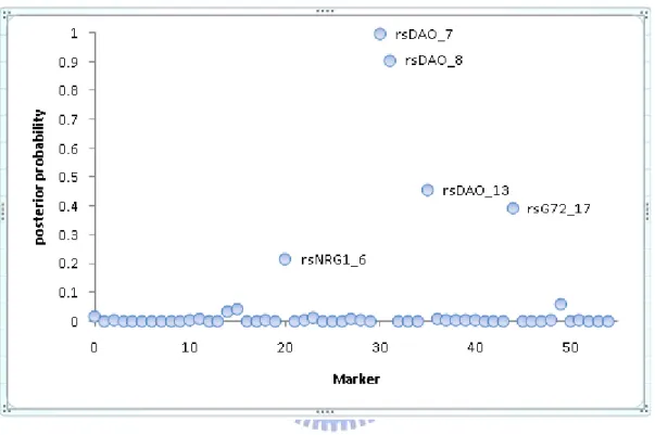
marker conditional on the current status of other markers iteratively and outputs the posterior probability that each marker and/or epistasis is associated with the disease. The method can be used either in a ‘pure’ bayesian sense or just as a tool to discover potential ‘hits’. For the former, one relies on the reported posterior probabilities to make inferential statements; as for the latter, one can take the reported hits and use another procedure to test whether these hits are statistically significant. The latter approach is more robust to model selection and prior assumptions (such as Dirichlet priors with arbitrary parameters) and is less prone to the slow mixing problem in the MCMC computational procedure. BEAM also proposes the B statistic to facilitate the

latter approach [7]. Figure 1 shows that an example of posterior probabilities of association for each marker by applying BEAM to our genotype-based data. We can see that two SNPs, rsDAO_7 and rsDAO_8, have a posterior probability above 0.5.

Figure 1. Example of posterior probabilities of association for each marker by applying BEAM to our genotype-based data. Two SNPs, rsDAO_7 and rsDAO_8, have a posterior probability above 0.5.

We use BEAM to detect both single-marker and epistasis associations in our genotype-based and haplotype-based data. The marker which had posterior probability that is associated with disease will be examined by B statistic. Then we can rank the association by the B statistic in one-way, two-way, and three-way interaction.

CART. Decision trees date back to the early 1960s with the work of Morgan and

Sonquist. Breiman and colleagues published the first comprehensive description of recursive partitioning methodology. As a powerful data analysis method, trees are used in many fields, such as epidemiology and medical diagnosis, and provide an alternative to more standard model-based regression techniques for multivariate analyses [1]. We use the S implementation [8] in the present study. Through binary recursive partitioning, a tree successively splits the data along the coordinate axes of the predictors such that, at each division, the resulting two subsets of data are as homogeneous as possible with respect to the response of interest. Deviance is a natural splitting criterion based on likelihood values.

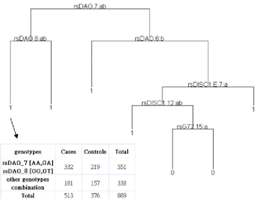
We used the S defaults in our study. That is, a node must include at least 10 observations and the minimum node deviance before the tree growing stops should be 1% of the root node. The subsets that are not further split are the terminal nodes. The SNP variables were considered as nominal categorical variables. We build the tree and then pruned it to a smaller tree using the deviance criteria (set the best size of tree equal to 5). Figure 2 is an example of applying CART to our genotype-based data. Investigating the tree terminal nodes provides a natural way to identify interaction. For example, we can calculate the chi-square statistic for each terminal node. Then we can rank the association by chi-square statistic. Note that we didn’t use CART to analyze our haplotype-based data because of computational limitation. In haplotype-based data, there are too many categories in block variables and factor predictor variables have a limit of levels in S.

Figure 2. Example of applying CART to genotype-based data

MDR. The MDR approach is a model-free and nonparametric approach that it does

not assume any particular genetic model and does not estimate any parameters. With MDR, multilocus genotypes are pooled into high risk and low risk groups, effectively reducing the dimensionality of the genotype predictors from N dimensions to one dimension. The new one-dimensional multilocus genotype variable is evaluated for its ability to classify and predict disease status using cross-validation and permutation testing. It identifies interactions through an exhaustive search, that is, it searches over all possible factor combinations to find combinations with an effect on an outcome

variable. We simply use the MDR default setting to detect gene-gene interactions in our two types of data. Note that we use the MDR v1.1.0 software in this study. There are some differences between this version and the original version described in the paper [10]. In the current version, interaction with the lowest classification error (average over the ten cross-validations) is selected as the best model in each k-way interaction. The interaction that maximizes the testing accuracy is selected as the final best overall model across all k-way models.

3.5 Cross-Validation (CV)

To evaluate the ability of a model to classify and predict a certain outcome variable, cross-validation is often used. We can use cross-validation to obtain the classification and prediction error of models relating predictors to disease status. We want to compare the abilities of prediction in these five methods. In present study, we randomly divided our genotype-based data into training set and testing set. The sample size of training set doubles that of testing set. For example, there are 513 cases and 376 controls in our data, the training set will contain 342 cases and 251 controls, and the testing set will contain 171 cases and 125 controls. We repeat this procedure 100 times to create 100 dataset. For each CV, we apply the five methods (Chi-square test, LRM, BEAM, CART, and MDR) to the training set and get the best model for one-way, two-way, and three-way interaction. Note that we only tested single marker effects and two-way interaction with Chi-square test and LRM since the investigation of three-way interactions could lead to computation problem. We use the training set to build a prediction rule for the best model. Like MDR, we compute the case-control ratio for each genotype combination, and partition the multi-locus genotypes into two subgroups labeled as high or low risk. When there is genotype combination contains no sample size in the training set, we ignore this combination and will not predict the

testing set individuals with this genotype combination. While the prediction rule is built, we can calculate the prediction error, the ratio of the number of individuals which be predicted wrong to the number of individuals which be predicted.

4 RESULTS

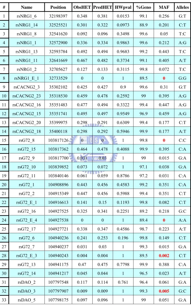
The data we used in present study contains 65 SNP markers and 890 individuals (514 cases and 376 controls). Table 1 shows that the information of each markers. It contains:

# is the marker number.

Name is the marker ID specified.

Position is the marker position specified (in base pair). ObsHET is the marker’s observed heterozygosity.

PredHET is the marker’s predicted heterozygosity (i.e. 2*MAF*(1-MAF)). HWpval is the Hardy-Weinberg equilibrium p value.

%Geno is the percentage of non-missing genotypes for this marker. MAF is the minor allele frequency for this marker.

Alleles are the major and minor alleles for this marker.

Using the criteria we described in the section of data quality control, we will exclude 10 SNPs: rsNRG1_E_1, rsG72_8, rsG72_E_4, rsG72_E_3, rsDAO_3, rsDAO_E_1, rsDAO_E_2, rsDISC1_E_3, rsDISC1_34, and rsDISC1_5. All because of the MAF is less than 0.01.

As we described in the section of study design, we used the Haploview software to define haplotype block. Figure 3 shows that the pair-wise LD plot and defined block in five genes. The deeper color means the stronger LD. There are five blocks (each block contains 2 SNPs) in DISC1, no block in NRG1, one block (contains 7 SNPs) in DAO, two blocks (one contains 3 SNPs and one contains 2 SNPs) in G72, and two blocks (each block contains 2 SNPs) in CACNG2. One block can be treated as one variable. Therefore, the haplotype-based data will have 39 variables (10 blocks and 29 SNPs).

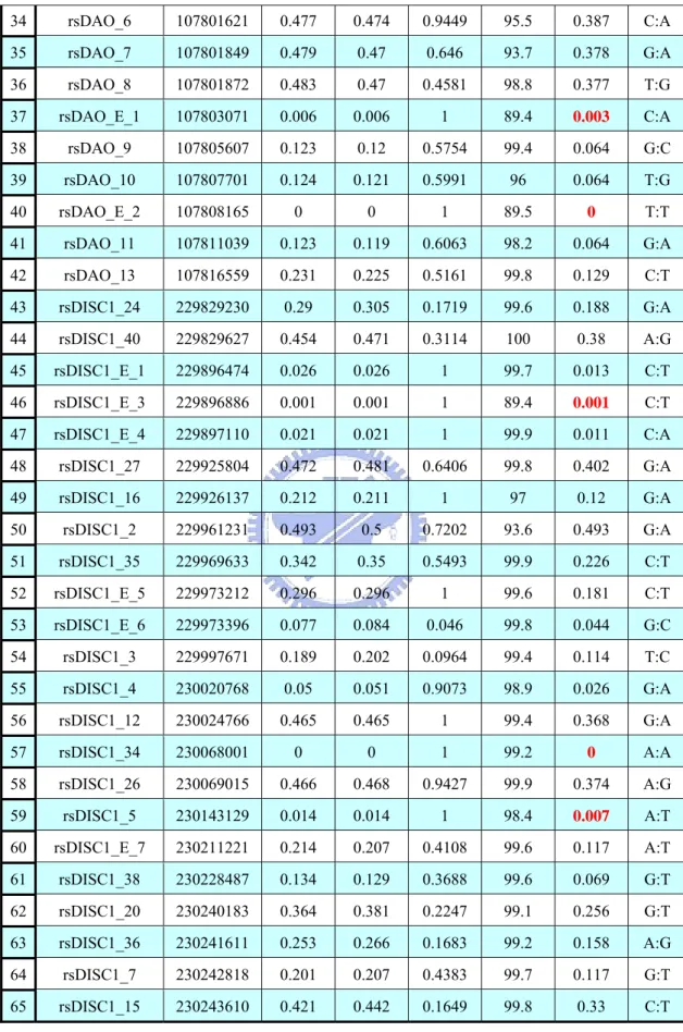
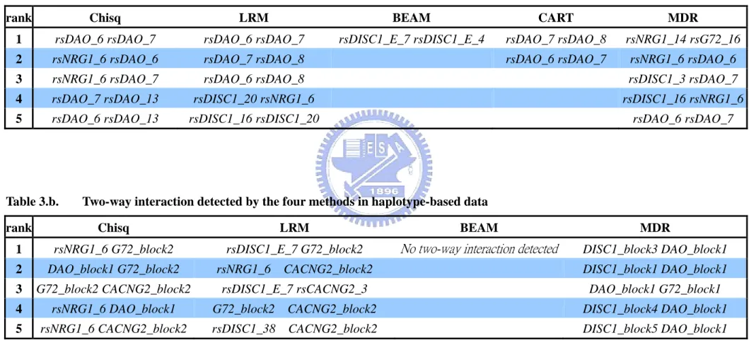
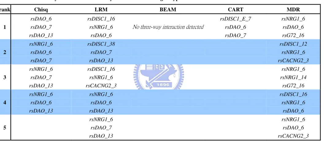
Our goal is to detect single marker effect, two-way and three-way interaction. We use the five methods and rank the association in our genotype-based and haplotype-based data. We showed the top five best models of single marker effects, two-way, and three-way interactions in table 2 to 4.

Single marker effects. In our genotype-based single marker effects study, chi-square

test, LRM, and BEAM identified that the SNP rsDAO_13 as the most significant marker. CART and MDR identified that the SNP rsDAO_7 as the most significant marker, which as the second most significant marker by chi-square test, LRM, and BEAM. And in the haplotype-based data, all methods shows that DAO_block1, which contains SNP rsDAO_13 and rsDAO_7, as the best model. It shows that DAO might be a significant gene with associated with schizophrenia.

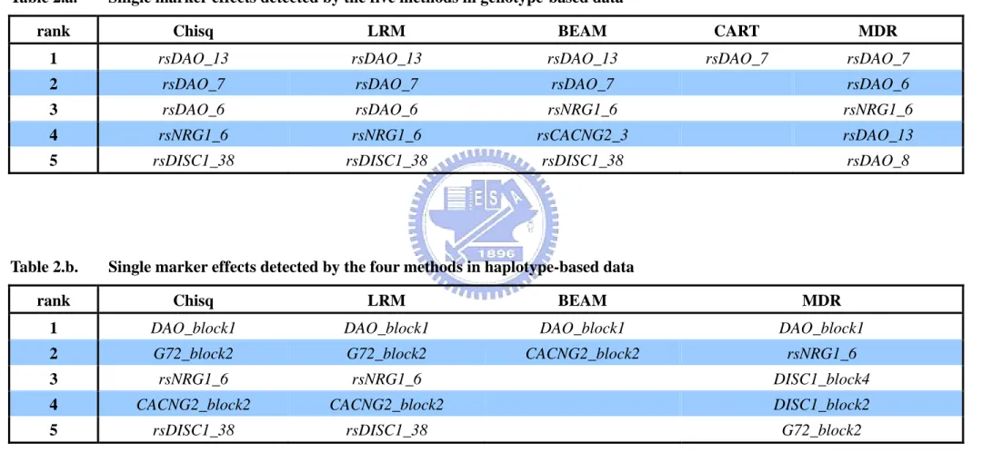
Two-way interaction. In genotype-based two-way interaction study, Chi-square,

LRM, and CART still shows that SNPs in DAO gene (rsDAO_6, rsDAO_7, and rsDAO_8) have two-way interaction, whereas BEAM and MDR did not detected. BEAM identified rsDISC1_E_7*rsDISC1_E_4 as two-way best model, and MDR identified rsNRG1_14*rsG72_16. It might because that Chi-square test, LRM, and CART require significant main effect to be detected before including interaction effects between factors. This is a major methodological limitation for situations where each marker has relatively small main effects but more substantial interactive effects. In these situations, using haplotype-base study might give more information. In haplotype-base study, Chi-square test and LRM detected that G72_block2 (which contains rsG72_16) has interaction effects with other SNP.

showed in table 4. Most of them were also detected by two-way interaction study. For example, rsDAO_6, rsDAO_7, rsG72_16, etc. In haplotype-based three-way interaction study, LRM faced numerical difficulties for estimating the model parameters since there are too many categories in block variables. Therefore, we did not propose the LRM three-way interaction in haplotype-based study.

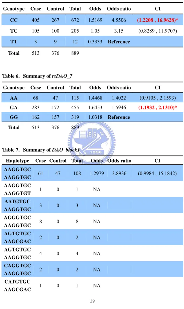
Odds ratio. In order to realize the relationship between genotype (haplotype) and

disease, we further calculate the odds ratio and its confidence interval for some candidate model (rsDAO_13, rsDAO_7, DAO_block1, and rsDAO_6*rsDAO_7). The results are showed in table 5 to 8. The genotype (haplotype) with minimum odds is considered as reference group. If the genotype with zero case or control, we didn’t calculate the odds ratio. We can see that the genotype CC of rsDAO_13 has a significant result, that is, the confidence interval of the odds ratio did not cover 1. Also, the genotype GA of rsDAO_7 has a significant result. In the model DAO_block1, there are also some haplotypes with significant odds ratio. Besides, there are many haplotypes with only affected individuals. Similar result also appeared in rsDAO_6*rsDAO_7.

Cross validation. By using the cross-validation procedure, we can get 100 best

models in each one-way, two-way, and three-way interaction along with each method. Using the prediction rule we described before, we can calculate prediction errors with each best model in each CV. We averaged the prediction errors across 100 CVs, which be showed in table 9. The box-plots of prediction error were also displayed in figure 4 to 6. In one-way interaction, BEAM shows best ability of prediction. However, the differences between each method are not too significant in box-plot. In two-way interaction, the traditional approach LRM shows that minimum prediction error, and

is much smaller than the others. BEAM seems to have worst prediction and has biggest variation. In three-way interaction, CART has the smaller prediction error but all three methods do not have good performance. Their prediction errors are too close to 0.5. A prediction error of 0.5 is what you expect if you were to predict case-control status by flipping a coin. It might because that our data did not contain a three-way interaction. We can see that the prediction error go up at two-way interaction and go down at three-way interaction in CART and MDR. Over-fitting might be the reason, that is, we add the false positives thus decreasing its predictive ability. It might be worth to note that the MDR has the smaller variation. This means that MDR is much stable than others.

5 CONCLUSION

Our aim of this study is to propose a methodological issue in detecting gene-gene interaction. We chose five commonly used methods and apply them to a schizophrenia data. Methods included traditional methods (chi-square test, LRM), Bayesian approach (BEAM), tree based model (CART), and combinatorial method (MDR). We also propose a haplotype-based study in gene-gene interaction. Using the haplotype based marker could give more information. If a haplotype block is highly associated with disease, the true disease gene (SNP) could be in the haplotype block. In the present study, we find that SNPs rsDAO_13 and rsDAO_7 have strong main effect. SNPs rsDAO_6, rsDAO_7, and rsG72_16 have strong gene-gene interaction effects. It can give the biologist a suggestion to type more markers in these genes for future analysis.

In order to compare the predictive ability of these methods, we used cross-validation approach and defined a prediction rule. LRM shows the best predictive ability in our data.

Table 1. Marker’s Information

# Name Position ObsHET PredHET HWpval %Geno MAF Alleles

1 rsNRG1_6 32198397 0.348 0.381 0.0153 99.1 0.256 G:T 2 rsNRG1_14 32525521 0.301 0.322 0.0973 88.9 0.201 C:T 3 rsNRG1_8 32541620 0.092 0.096 0.3498 99.6 0.05 T:C 4 rsNRG1_1 32572900 0.336 0.334 0.9863 99.6 0.212 A:G 5 rsNRG1_13 32593784 0.492 0.494 0.9683 99.2 0.443 T:C 6 rsNRG1_11 32641669 0.467 0.482 0.3734 99.1 0.405 A:T 7 rsNRG1_2 32705627 0.127 0.133 0.3115 99.8 0.072 T:C 8 rsNRG1_E_1 32733529 0 0 1 89.5 0 G:G 9 rsCACNG2_3 35302102 0.425 0.427 0.9 99.6 0.31 G:T 10 rsCACNG2_23 35318530 0.459 0.478 0.2592 99 0.395 A:G 11 rsCACNG2_16 35351483 0.477 0.494 0.3322 99.4 0.447 A:G 12 rsCACNG2_15 35351741 0.495 0.497 0.9549 96.9 0.459 A:G 13 rsCACNG2_20 35399975 0.298 0.291 0.6309 99.4 0.177 C:T 14 rsCACNG2_18 35400118 0.298 0.292 0.5946 99.9 0.177 A:T 15 rsG72_8 103817126 0 0 1 99.8 0 C:C 16 rsG72_15 103817362 0.464 0.478 0.4088 99.9 0.395 C:A 17 rsG72_9 103817700 0.031 0.03 1 99 0.015 G:A 18 rsG72_10 103839852 0.073 0.072 1 97.1 0.038 G:A 19 rsG72_11 103840146 0.061 0.059 0.8786 97.2 0.031 C:A 20 rsG72_1 104908896 0.443 0.456 0.4583 99.2 0.351 C:A 21 rsG72_2 104915349 0.447 0.456 0.5988 99.4 0.351 C:T 22 rsG72_E_1 104916613 0.141 0.15 0.1193 99.8 0.082 C:T 23 rsG72_16 104927525 0.325 0.341 0.2251 89.2 0.218 G:C 24 rsG72_E_4 104927538 0 0 1 89.4 0 A:A 25 rsG72_17 104927721 0.338 0.347 0.4586 98.7 0.223 A:T 26 rsG72_6 104940236 0.241 0.253 0.196 99.8 0.149 C:T 27 rsG72_7 104940237 0.031 0.03 1 99.3 0.015 G:A 28 rsG72_E_3 104940243 0.004 0.004 1 89.5 0.002 C:T 29 rsG72_13 104941175 0.47 0.475 0.7798 99.9 0.388 C:A 30 rsG72_14 104941217 0.045 0.044 1 96.5 0.023 A:T 31 rsDAO_2 107797548 0.117 0.114 0.761 96.4 0.061 G:A 32 rsDAO_3 107797907 0.009 0.009 1 99.3 0.005 G:C 33 rsDAO_5 107798175 0.097 0.096 1 99 0.051 G:A

Table 1. Marker’s Information (Cont’d) 34 rsDAO_6 107801621 0.477 0.474 0.9449 95.5 0.387 C:A 35 rsDAO_7 107801849 0.479 0.47 0.646 93.7 0.378 G:A 36 rsDAO_8 107801872 0.483 0.47 0.4581 98.8 0.377 T:G 37 rsDAO_E_1 107803071 0.006 0.006 1 89.4 0.003 C:A 38 rsDAO_9 107805607 0.123 0.12 0.5754 99.4 0.064 G:C 39 rsDAO_10 107807701 0.124 0.121 0.5991 96 0.064 T:G 40 rsDAO_E_2 107808165 0 0 1 89.5 0 T:T 41 rsDAO_11 107811039 0.123 0.119 0.6063 98.2 0.064 G:A 42 rsDAO_13 107816559 0.231 0.225 0.5161 99.8 0.129 C:T 43 rsDISC1_24 229829230 0.29 0.305 0.1719 99.6 0.188 G:A 44 rsDISC1_40 229829627 0.454 0.471 0.3114 100 0.38 A:G 45 rsDISC1_E_1 229896474 0.026 0.026 1 99.7 0.013 C:T 46 rsDISC1_E_3 229896886 0.001 0.001 1 89.4 0.001 C:T 47 rsDISC1_E_4 229897110 0.021 0.021 1 99.9 0.011 C:A 48 rsDISC1_27 229925804 0.472 0.481 0.6406 99.8 0.402 G:A 49 rsDISC1_16 229926137 0.212 0.211 1 97 0.12 G:A 50 rsDISC1_2 229961231 0.493 0.5 0.7202 93.6 0.493 G:A 51 rsDISC1_35 229969633 0.342 0.35 0.5493 99.9 0.226 C:T 52 rsDISC1_E_5 229973212 0.296 0.296 1 99.6 0.181 C:T 53 rsDISC1_E_6 229973396 0.077 0.084 0.046 99.8 0.044 G:C 54 rsDISC1_3 229997671 0.189 0.202 0.0964 99.4 0.114 T:C 55 rsDISC1_4 230020768 0.05 0.051 0.9073 98.9 0.026 G:A 56 rsDISC1_12 230024766 0.465 0.465 1 99.4 0.368 G:A 57 rsDISC1_34 230068001 0 0 1 99.2 0 A:A 58 rsDISC1_26 230069015 0.466 0.468 0.9427 99.9 0.374 A:G 59 rsDISC1_5 230143129 0.014 0.014 1 98.4 0.007 A:T 60 rsDISC1_E_7 230211221 0.214 0.207 0.4108 99.6 0.117 A:T 61 rsDISC1_38 230228487 0.134 0.129 0.3688 99.6 0.069 G:T 62 rsDISC1_20 230240183 0.364 0.381 0.2247 99.1 0.256 G:T 63 rsDISC1_36 230241611 0.253 0.266 0.1683 99.2 0.158 A:G 64 rsDISC1_7 230242818 0.201 0.207 0.4383 99.7 0.117 G:T 65 rsDISC1_15 230243610 0.421 0.442 0.1649 99.8 0.33 C:T

Table 2.a. Single marker effects detected by the five methods in genotype-based data

rank Chisq LRM BEAM CART MDR

1 rsDAO_13 rsDAO_13 rsDAO_13 rsDAO_7 rsDAO_7

2 rsDAO_7 rsDAO_7 rsDAO_7 rsDAO_6

3 rsDAO_6 rsDAO_6 rsNRG1_6 rsNRG1_6

4 rsNRG1_6 rsNRG1_6 rsCACNG2_3 rsDAO_13

5 rsDISC1_38 rsDISC1_38 rsDISC1_38 rsDAO_8

Table 2.b. Single marker effects detected by the four methods in haplotype-based data

rank Chisq LRM BEAM MDR

1 DAO_block1 DAO_block1 DAO_block1 DAO_block1

2 G72_block2 G72_block2 CACNG2_block2 rsNRG1_6

3 rsNRG1_6 rsNRG1_6 DISC1_block4

4 CACNG2_block2 CACNG2_block2 DISC1_block2

Table 3.a. Two-way interaction detected by the five methods in genotype-based data

rank Chisq LRM BEAM CART MDR

1 rsDAO_6 rsDAO_7 rsDAO_6 rsDAO_7 rsDISC1_E_7 rsDISC1_E_4 rsDAO_7 rsDAO_8 rsNRG1_14 rsG72_16

2 rsNRG1_6 rsDAO_6 rsDAO_7 rsDAO_8 rsDAO_6 rsDAO_7 rsNRG1_6 rsDAO_6

3 rsNRG1_6 rsDAO_7 rsDAO_6 rsDAO_8 rsDISC1_3 rsDAO_7

4 rsDAO_7 rsDAO_13 rsDISC1_20 rsNRG1_6 rsDISC1_16 rsNRG1_6

5 rsDAO_6 rsDAO_13 rsDISC1_16 rsDISC1_20 rsDAO_6 rsDAO_7

Table 3.b. Two-way interaction detected by the four methods in haplotype-based data

rank Chisq LRM BEAM MDR

1 rsNRG1_6 G72_block2 rsDISC1_E_7 G72_block2 No two-way interaction detected DISC1_block3 DAO_block1

2 DAO_block1 G72_block2 rsNRG1_6 CACNG2_block2 DISC1_block1 DAO_block1

3 G72_block2 CACNG2_block2 rsDISC1_E_7 rsCACNG2_3 DAO_block1 G72_block1

4 rsNRG1_6 DAO_block1 G72_block2 CACNG2_block2 DISC1_block4 DAO_block1

Table 4.a. Three-way interaction detected by the five methods in genotype-based data

rank Chisq LRM BEAM CART MDR

1 rsDAO_6 rsDAO_7 rsDAO_13 rsDISC1_16 rsNRG1_6 rsDAO_6

No three-way interaction detected

rsDISC1_E_7 rsDAO_6 rsDAO_7 rsNRG1_6 rsDAO_6 rsG72_16 2 rsNRG1_6 rsDAO_6 rsDAO_7 rsDISC1_38 rsDAO_7 rsDAO_13 rsDISC1_12 rsNRG1_6 rsCACNG2_3 3 rsNRG1_6 rsDAO_7 rsDAO_13 rsDISC1_16 rsNRG1_6 rsCACNG2_3 rsNRG1_6 rsNRG1_14 rsG72_16 4 rsNRG1_6 rsDAO_6 rsDAO_13 rsNRG1_6 rsDAO_6 rsDAO_13 rsDISC1_16 rsNRG1_6 rsDAO_6 5 rsNRG1_6 rsDAO_7 rsDAO_13 rsNRG1_6 rsDAO_6 rsCACNG2_3

rank Chisq BEAM MDR

1

G72_block2 rsNRG1_6 CACNG2_block2

No three-way interaction detected

DISC1_block1 DISC1_block3 DAO_block1 2 DAO_block1 G72_block2 rsNRG1_6 DISC1_block1 DAO_block1 G72_block1 3 DAO_block1 rsNRG1_6 CACNG2_block2 DISC1_block1 DISC1_block4 DAO_block1 4 DAO_block1 G72_block2 CACNG2_block2 DISC1_block3 DISC1_block4 DAO_block1 5 DISC1_block2 DISC1_block4 DAO_block1

Table 5. Summary of rsDAO_13

Genotype Case Control Total Odds Odds ratio CI

CC 405 267 672 1.5169 4.5506 (1.2208 , 16.9628)*

TC 105 100 205 1.05 3.15 (0.8289 , 11.9707)

TT 3 9 12 0.3333 Reference

Total 513 376 889

Table 6. Summary of rsDAO_7

Genotype Case Control Total Odds Odds ratio CI

AA 68 47 115 1.4468 1.4022 (0.9105 , 2.1593) GA 283 172 455 1.6453 1.5946 (1.1932 , 2.1310)*

GG 162 157 319 1.0318 Reference Total 513 376 889

Table 7. Summary of DAO_block1

Haplotype Case Control Total Odds Odds ratio CI AAGGTGC AAGGTGC 61 47 108 1.2979 3.8936 (0.9984 , 15.1842) AAGGTGC AAGGTGT 1 0 1 NA AATGTGC AAGGTGC 3 0 3 NA AGGGTGC AAGGTGC 8 0 8 NA AGTGTGC AAGCGAC 2 0 2 NA AGTGTGC AAGGTGC 4 0 4 NA CAGGTGC AAGGTGC 2 0 2 NA CATGTGC AAGCGAC 1 0 1 NA

Table 7. Summary of DAO_block1 (Cont’d)

Haplotype Case Control Total Odds Odds ratio CI CGTCGAC AAGCGAC 1 0 1 NA CGTCGAC AAGGTGC 27 18 45 1.5 4.5 (1.0701 , 18.9238)* CGTCGAC AGTGTGC 1 0 1 NA CGTCGAC CATGTGC 2 0 2 NA CGTCGAC CGTCGAC 1 0 1 NA CGTCGAC CGTGTGC 22 16 38 1.375 4.125 (0.9611 , 17.7043) CGTCGAC CGTGTGT 6 4 10 1.5 4.5 (0.7300 , 27.7401) CGTCGGC AAGGTGC 0 2 2 NA CGTCTAC AAGGTGC 2 1 3 2 6 (0.3901 , 92.2820) CGTCTAC AGGGTGC 1 0 1 NA CGTGGGC AAGGTGC 1 0 1 NA CGTGTGC AAGGTGC 172 113 285 1.5221 4.5664 (1.2101 , 17.2320)* CGTGTGC AGGGTGC 1 0 1 NA CGTGTGC AGTGTGC 10 0 10 NA CGTGTGC CATGTGC 10 0 10 NA CGTGTGC CGTGTGC 73 70 143 1.0429 3.1286 (0.8133 , 12.0342) CGTGTGC CGTGTGT 40 56 96 0.7143 2.1429 (0.5455 , 8.4179)

Table 7. Summary of DAO_block1 (Cont’d)

Haplotype Case Control Total Odds Odds ratio CI CGTGTGT AAGCGAC 2 2 4 1 3 (0.2845 , 31.6342) CGTGTGT AAGGTGC 45 36 81 1.25 3.75 (0.9451 , 14.8792) CGTGTGT AATGTGC 1 0 1 NA CGTGTGT AGGGTGC 1 0 1 NA CGTGTGT AGTGTGC 3 2 5 1.5 4.5 (0.4909 , 41.2495) CGTGTGT CATGTGC 6 0 6 NA CGTGTGT CGTGTGT 3 9 12 0.3333 Reference Total 513 376 889

Table 8. Summary of rsDAO_6*rsDAO_7

Genotype Case Control Total Odds Odds ratio CI

AA*AA 65 47 112 1.3830 1.4784 (0.9537 , 2.2916) AA*GA 14 0 14 NA AA*GG 0 0 0 NA AC*AA 3 0 3 NA AC*GA 251 172 423 1.4593 1.5599 (1.1577 , 2.1019)* AC*GG 17 2 19 8.5 9.0862 (2.0630 , 40.0185)* CC*AA 0 0 0 NA CC*GA 18 0 18 NA CC*GG 145 155 300 0.9355 Reference Total 513 376 889

Table 9. Average prediction error across 100 CVs

Chisq LRM BEAM CART MDR one-way 0.471283784 0.476047297 0.471148649 0.486824324 0.473783784

two-way 0.464207618 0.448881209 0.488123798 0.477674915 0.470942832

Figure 3.a. Haplotype block in DISC1

Figure 3.c. Haplotype block in DAO

Figure 3.e. Haplotype block in CACNG2