利用藥物化學特徵和統計學習建構藥物負向事件預測模型

國

立

交

通

大

學

統計學研究所

碩士論文

利用藥物化學特徵和統計學習建構藥物負向事件預測模型

Prediction for Adverse Drug Events by

Chemical

Descriptors and Statistical Learning

研 究 生：吳宜靜

指導教授：盧鴻興 教授

利用藥物化學特徵和統計學習建構藥物負向事件預測模型

Prediction for Adverse Drug Events by

Chemical Descriptors and

Statistical Learning

研究生：吳宜靜

Student：Yi-Jing Wu

指導教授：盧鴻興 博士 Advisor：Dr. Henry Horng-Shing Lu

國 立 交 通 大 學

統 計 學 研 究 所

碩

士

論

文

A Thesis

Submitted to Institute of Statistics

College of Science

National Chiao Tung University

In Partial Fulfillment of the Requirements

For the Degree of

Master

in

Statistics

June 2012

Hsinchu, Taiwan, Republic of China

利用藥物化學特徵和統計學習建構藥物負向事件預測模型

研究生：吳宜靜

指導教授：盧鴻興 教授

國立交通大學統計學研究所

摘

要

當藥物成分進入人體後，產生複雜的擾動效應稱為藥效。藥效可分為主要治療藥效和額外

的效果，而

藥物不良反應事件

是額外效果的一部分。

每個藥物成分都是一種化合物，由其

化學式可以得到化學資訊特徵。基於藥物在人體系統中產生的生物擾動與其化學結構有關

的假設，我們檢視上市藥物的藥物不良反應事件與其化學資訊特徵之間的關聯。在本研究

中，我們使用決策樹方法指認出與 1384 個藥物不良反應事件的相關化學資訊特徵，並設計

一套自動分析流程。針對我們選定的 35 個有興趣的藥物不良反應事件可以得到模型十折交

叉驗證正確率高於 80%，例如: 糖尿病（87.1%），急性腎功能衰竭（91.0%）和腎功能不全

（94.6%）。

Prediction for Adverse Drug Events by Chemical Descriptors

and Statistical Learning

Student：Yi-Jing Wu

Advisor：Dr. Henry Horng-Shing Lu

Institute of Statistics

National Chiao Tung University

Hsinchu, Taiwan

Abstract

In addition to the medicine treatment effect, side effects are complex undesired phenomena due to

the bio-activity of pharmaceutical compound. For each compound, the chemistry informatics can

delineate its intrinsic chemical formula into chemistry informatics features. Based on the

assumption that the chemical structure is critical to the biological perturbation in the human

system, we investigate different adverse drug events with associated chemistry informatics

features of marketed drugs. In this research, we identify 1,384 ADEs with corresponding

associated chemistry informatics features by decision tree. With an automatic analysis workflow,

we can obtain a concordant drug subset with satisfying 10-fold cross-validation accuracy. The

accuracy of selected 35 ADEs in the test experiment is higher than 80%. For example, there are

three ADEs of interest and their accuracy: Diabetes Mellitus (0.871), Renal Failure Acute (0. 910)

and Renal Impairment (0. 946).

誌 謝

兩年碩士生涯雖然短暫但是收穫卻不少。這兩年能夠有所成果，

首先必須感謝我的指導教授─盧鴻興教授，感謝您在論文上、

課業上以及生活上不厭其煩地指導與幫助。其次，感謝口試委

員許文郁教授、王秀瑛教授以及謝文萍教授辛苦審查，並給指

導和建議使論文更加完善。

也必須感謝交大統計所所有的老師、郭姐和劉小姐，除了提供

我們良好的學習環境，讓我在碩士兩年學到了許多知識外，平

日給予的關懷與幫助讓我們能夠無憂無慮地學習。

再來要感謝所有交大統計所 99 級的同學們，因為有你們的一同

努力與分享，在兩年碩士生活中一起歡笑一起哭，讓我這兩年

的學習過程多了更多的調味劑。

最後，我要感謝我的家人，謝謝他們在我學習生涯中無論是遇

到挫折或是難過都給予我百分百的支持，使我能夠在學習過程

中完全無後顧之憂。

吳宜靜 謹誌于

國立交通大學統計學研究所

中華名國一百零一年六月

Contents

1. 

Introduction... 1 

1.1. 

Background ... 1 

1.2. 

Literature Review ... 5 

1.3. 

Purpose of Research ... 6 

2. 

Method ... 7 

2.1. 

Materials ... 7 

2.2. 

Data Analysis ... 9 

2.3. 

Research Design ... 16 

3. 

Result ... 20 

3.1. 

Compare the performance by using different types of chemical feature sets. ... 20 

3.2. 

Select concordant drugs and then analyze the relation between chemical compounds

and ADE under the regular condition ... 23 

4. 

Discussion and Conclusions ... 31 

4.1. 

Discussion ... 31 

4.2. 

Conclusion ... 33 

4.3. 

Recommendation for Future Research ... 34 

Reference: ... 35 

List of Figures

Figure 1.1 The drug-metabolizing capability.

 ... 3 

Figure 1.2 The instance about the therapeutic drug targets existing in multiple cell and

tissue types.

 ... 4 

Figure 1.3 The main purpose of our research.

 ... 6 

Figure 2.1 Flow chart for pre-processing work.

 ... 11 

Figure 2.2 Workflow about the automatic clustering analysis.

 ... 16 

Figure 2.3 The instance of concordant drug subset by concordant clustering analysis.

 .... 17 

Figure 2.4 The structure of clustering generated from the automatic clustering analysis.

 18 

Figure 2.5 Flow chart of our research.

 ... 19 

Figure 3.1(a) The result of the first question in the first stage.

 ... 21 

Figure 3.1(b) The result of the second question in the first stage.

 ... 21 

Figure 3.1(c) The result of the third question in the first stage.

... 22 

Figure 3.2 Comparison of the IDT and SGDT for each ADEs of interest.

 ... 23 

Figure 3.3(a) Using the prediction accuracy to compare the IDT and SGDT for each

ADEs of interest.

 ... 24 

Figure 3.3(b) Using the ratio between prediction accuracy and guess rate to compare the

IDT and SGDT for each ADEs of interest.

 ... 25 

Figure 3.4 This is similarity guided decision tree of diabetes mellitus.

 ... 26 

Figure 3.5 This is similarity guided decision tree of renal failure acute.

 ... 28 

Figure 3.6 This is similarity guided decision tree of renal impairment.

 ... 30 

Figure 4.1 Using a graph to explain why an unselected drug is concordant

to the most similar selected drug.

 ... 32 

List of Tables

Table 2.1 This is an introduction about ASCII files.

 ... 8 

Table 2.2 A comprehensive list of chemical descriptors used in this study.

 ... 9 

Table 2.3(a) 1411 approval drugs’ information.

 ... 11 

Table 2.3(b) List of what information are contained in DRUGyyQq.txt.

 ... 12 

Table 2.3(c) List of what information are contained in REACyyQq.txt.

 ... 12 

Table 3.1 The chemical description of features we used in the diabetes mellitus prediction

model.

 ... 26 

Table 3.2 The chemical description of features we used in the renal failure acute

prediction model.

 ... 27 

Table 3.3 The chemical description of features we used in the renal impairment.

 ... 28 

Table 4.1 Show the number of unselected drugs and selected drugs for the two ADEs of

interest..

 ... 31 

Table 4.2 Show the approval date of the two unselected drugs and two “the most similar”

selected drugs..

 ... 32 

List of Notation and Abbreviations

Abbreviation Terminology

ADE

Adverse Drug Event

FDA

Food and Drug Administration

AERS

Adverse Event Reporting System

HIV

MedDRA

Medical Dictionary for Regulatory

Activities

CDK

Chemistry Development Kit

ISR

CV

Cross-Validation

IDT

Initial Decision Tree

1. Introduction

1.1. Background

Modern medicine provides more sanative treatment due to the improvement in

pharmaceutical equipment. However, this achievement gives rise to some potential

danger in drug usage. An UK national analysis indicates that each year adverse drug

reactions are responsible for 5% hospital admission which cost approximately 0.5 billion

pounds per year. Besides, fatal adverse drug reactions account for approximately 3% of

all death in the general population [1]. The research of drug monitoring reveals that

adverse drug reactions can turn into social cost.

The market drugs are required to show indications on the package or in the

instructions leaflet. If the pharmacists want drugs to be approved for sale, they must

report clinical results to the Food and Drug Administration (FDA). The clinical trial

should control some of the confounding variable effect, such as, age, gender, or changes

in hormone level. Subjects of the clinical trial are randomly assigned into two groups in

double blind procedure. Subjects in the experiment group are given the drug, and the

others in control group are receiving placebo. The main purpose of the clinical trial is to

confirm the principal treatment effect and the secondary purpose is to find possible

adverse reactions.

Side effect is a usual term for the negative consequence of adverse drug reaction.

And the medical record about side effect or adverse drug reaction is a report of adverse

drug event (ADE). Since 2004, the FDA set up a Pharmacovigilance system to collect the

negative consequence of market drug reports from the health professionals and patients.

All the information about adverse drug events is recorded in adverse effect reporting

system (AERS).

Besides, FDA is asked to do some analysis related to adverse drug effects and

provides these results to the public. If FDA find some adverse drug effects are not listed

on the package or in the instructions leaflet, FDA will ask pharmaceutical company to

provide inspection reports, and may have three possible procedures:

i.

The pharmaceutical company should list “new” adverse effects on the package

or in the instructions leaflet.

ii.

The pharmaceutical company should indicate the eligibility of patients on the

package or in the instructions leaflet.

iii.

In the worst case, the drugs will be removed from the shelves.

We notice the importance to investigate adverse drug events. In consequence, we

search the literatures about the hidden risk of approval drugs and start the following

research in this thesis for the drug safety issue.

“The occurrence of drug side effect” is one of the most popular topics in the field of

modern medicine. Nowadays, experts and scholars have proposed the possible causes of

adverse drug effects into four categories [2]:

(1)

Adverse events related to the therapeutic effects of drugs:

The first category of adverse drug effects occurs when the therapeutic effects have

other additional negative consequences. Generally, these drug side effects occur as the

concentration of medication is higher than required for beneficial drug effects. The drug

metabolism variation is related to several enzyme activities. The required dose of drug

might be different among people due to the individual genomic factor.

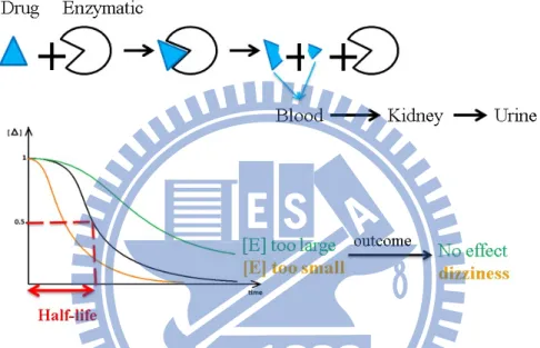
In general case, drugs are catalyzed by some enzymes in the liver. The drug effects

in human system will become vanished as the time passed. After enzymatic reaction, the

catalyzed drug waste will be transported to the kidney and then excreted into urine.

However, the enzyme activity is diverse among people. If the enzyme activity is higher;

that is, the rate of metabolism increases, then the time of drugs functioning in vivo is

shorter than average. Therefore, it can result in less treatment effect. However, if the

enzyme activity is lower; that is, the rate of metabolism decreases, then the time of drugs

functioning in vivo is longer than average. Thus, it results in higher treatment effect and

adverse drug effect (Figure 1.1).

For example, anticoagulant (Warfarin) is to inhibit vitamin K epoxide reductase

(VKOR). However, if the concentration of medication in vivo is higher than that required

for beneficial drug effect, this will result in over-inhibited clotting, which may lead to

hemorrhagic stroke.

Figure 1.1: This figure shows that the drug-metabolizing capability. The black curve

denotes the general case, the orange curve denotes the lower enzyme

activity, and the green curve denotes the higher enzyme activity.

(2)

The therapeutic drug targets existing in multiple cell and tissue

types:

The second category of adverse drug events occurs when a drug’s target (a specific

protein) serves multiple functions in different tissues of the body.

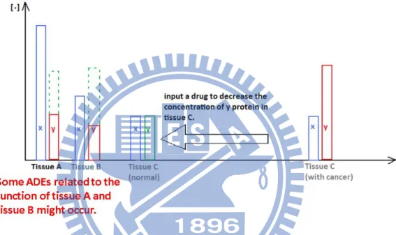
For illustration, given three different tissues, A, B, and C, all of them contain two

proteins x and y and their corresponding expression level in normal case. If the

expression of protein y in tissue C is higher, tissue C becomes cancerous. And the design

a chemical compound, which can hydrolyze protein y or block its bio-activity, aims to

drug inhibits protein y in tissue C, as well as in tissue A and tissue B. Thus, it causes the

function of protein y in tissue A and tissue B becomes less than normal, which we

consider as a possible scenario of the cause of adverse drug effect (Figure 1.2).

In real case, Morphine is designed to achieve analgesia by binding with µ-opioid

receptors in the brain. However, it may affect the same type of opiate receptors in the

intestines, which inhibits peristalsis.

Figure 1.2: Initially, we want to regulate tissue C by inputting an anti-cancer drug. The

function of the anti-cancer drug inhibits the protein y in tissue C. It as well as

inhibits protein y in tissue A and tissue B at the same time. Thus, ADEs will

be resulted.

(3)

Adverse drug events mediated by off-targets of a drug:

The third category of adverse drug events occurs when one drug interferes with

other unexpected proteins or pathways. This category is different from the second

category. The former considers that one drug affects single protein among more than one

tissue. The protein or pathway that the drug intends to function is called “drug-target”,

and the drug affecting unexpected proteins or pathway is called “off-target”. It should be

mentioned that the off-target will be another scenario of side effects.

For example, Delavirdine, HIV reverse transcriptase inhibitor, not only inhibits the

reverse transcriptase of HIV, but also interacts with histamine H4 receptor, which will

result in severe rash.

(4)

Mixture of several drug side effects:

The fourth category is a mixture of the adverse drug events in above three categories.

For example, Domperidone is designed to promote gastrointestinal motility, but also

inhibits the human Ether-à-go-go-Related Gene K+ channels (HERG K+ channels),

which will result in cardiac arrhythmias.

1.2. Literature Review

Hammann et.al has reported a set of ADE prediction models with high prediction

accuracy in chemistry and pharmaceutical field [3]. This research has been published in a

journal of nature group (Clinical Pharmacology & Therapeutics, with impact factor

6.961*).

In this article, they state the relation between the drug chemical features and the

ADE as the perturbed “human body functioning mechanism”.

In the study, they used decision tree to establish the association between drugs’

chemical features and ADEs. They analyzed four kinds of ADEs, allergy, central nervous

system (CNS), hepatotoxicity and nephrotoxicity. The importance of drug chemical

descriptors can be revealed, because the proposed the four ADE prediction models

achieved high prediction accuracy rate, 89.74%, 90.22%, 88.68%, and 78.94%,

respectively.

However, in the four ADE models, only few market drugs are considered. The

number of market drugs of each ADE is 164, 286, 334, and 338 respectively. In addition,

they do not clearly explain how to select the “drug subset” from the initial drug set (507

drugs) for each ADE by using the reporting frequency threshold.

1.3. Purpose of Research

Although a majority of patients can reach the most of efficacy after taking medicine,

still some patients will experience some particular side effects or adverse events.

Furthermore, some side effects will result in serious injury in patients, such as

hepatotoxicity and rhabdomyolysis which lead to acute cardiac death. In our study, we

want to predict more ADEs based on Adverse Event Reporting System (AERS) and more

market drugs. Our goals of the present study are to expand the chemical descriptors

database, and to develop an automatic concordant analysis to obtain an explainable drug

subset in the feature space. In this research, we aim to determine the chemical, physical,

and structural properties of compounds that are associated with certain ADE.

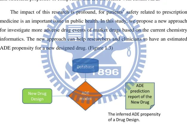
The impact of this research is profound, for patients’ safety related to prescription

medicine is an important issue in public health. In this study, we propose a new approach

for investigate more adverse drug events of market drugs based on the current chemistry

informatics. The new approach can help researchers and clinicians to have an estimated

ADE propensity for a new designed drug. (Figure 1.3)

2. Method

2.1. Materials

Adverse drug report

AERS is a computerized information database [4]. It is a monitoring program

designed to support the safety of drugs on the shelf. When we download the AERS

database, we can get two kinds of formats, one is SGML and the other is ASCII. ASCII

data files contain seven different types of folders and each folder contains the relative

information of adverse drug events. For example, the “REAC” folder contains several

data files (notated: REACyyQq.txt), and each file contains the adverse events of each

drug. Table 2.1 lists each folder in detail. We use the ASCII data files which are collected

from the first quarter of 2004 to the fourth quarter of 2010 to get the number of reports

for each drug and each ADE.

In order to get the ADE list, we download the pt.asc file from the Medical

Dictionary for Regulatory Activities (MedDRA). MedDRA is a medical dictionary and is

used to classify the information about adverse event associated with the use of

biopharmaceuticals and other medical products. Because the drugs’ names which

recorded in the AERS database are not always generic names, we need a comprehensive

list of drugs’ names. Therefore, we find the corresponded generic name, brand names,

and synonyms of each approval drug in the DrugBank database. The DrugBank database

combines the complete information about drug target and detailed drug [5].

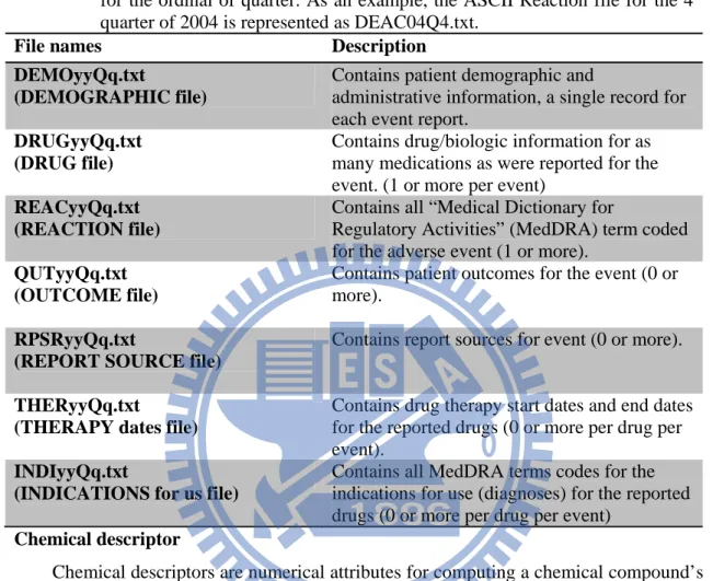
Table 2.1: In the ASCII format, file names have the format <file-descriptor>yyQq, where

<file-descriptor> is a 4-letter abbreviation of the data source, “yy” is a 2-digit

identifier for the year, “Q” stands for the quarter, and “q” is a 1-digit identifier

for the ordinal of quarter. As an example, the ASCII Reaction file for the 4

quarter of 2004 is represented as DEAC04Q4.txt.

File names

Description

DEMOyyQq.txt

(DEMOGRAPHIC file)

Contains patient demographic and

administrative information, a single record for

each event report.

DRUGyyQq.txt

(DRUG file)

Contains drug/biologic information for as

many medications as were reported for the

event. (1 or more per event)

REACyyQq.txt

(REACTION file)

Contains all “Medical Dictionary for

Regulatory Activities” (MedDRA) term coded

for the adverse event (1 or more).

QUTyyQq.txt

(OUTCOME file)

Contains patient outcomes for the event (0 or

more).

RPSRyyQq.txt

(REPORT SOURCE file)

Contains report sources for event (0 or more).

THERyyQq.txt

(THERAPY dates file)

Contains drug therapy start dates and end dates

for the reported drugs (0 or more per drug per

event).

INDIyyQq.txt

(INDICATIONS for us file)

Contains all MedDRA terms codes for the

indications for use (diagnoses) for the reported

drugs (0 or more per drug per event)

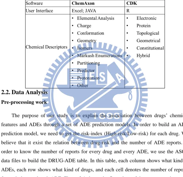
Chemical descriptor

Chemical descriptors are numerical attributes for computing a chemical compound’s

structure. These include elemental analysis, charge analysis, geometry, partitioning

coefficient and other characteristics. Some of chemical descriptors include large

information about measures of molecular connectivity, connectivity indexes.

There are two sources to get chemical descriptors, one is ChemAxon, and the other

is Chemistry Development Kit (CDK). ChemAxon is a providing chemical software

development platform for characterizing chemical structures and substructures [6].

Additional chemical descriptors are calculated by using the open-source cheminformatics

package, CDK

[7]. This package allows users to access functionality by a Java

framework for cheminformatics including load molecules, evaluate fingerprints, and

calculate molecular descriptors, etc.

A list of chemical descriptors used in our study is given in Table 2.2. It is

worth

noting that for some chemical descriptors they do not have only one

chemical feature. A

comprehensive list of chemical features used in this study is given in Appendix A.

Table 2.2: This is a comprehensive list of chemical descriptors we used in this study.

There are two sources of chemical descriptors, one is ChemAxon and the

other is CDK.

2.2. Data Analysis

Pre-processing work

The purpose of our study is to explain the association between drugs’ chemical

features and ADEs through a set of ADE prediction models. In order to build an ADE

prediction model, we need to get the risk-index (High-risk/Low-risk) for each drug. We

believe that it exist the relation between drug-risk and the number of ADE reports. In

order to know the number of reports for every drug and every ADE, we use the ASCII

data files to build the DRUG-ADE table. In this table, each column shows what kind of

ADEs, each row shows what kind of drugs, and each cell denotes the number of reports

for each drug and each ADE. Figure 2.1 shows the flow chart of the pre-processing work

and Table 2.3 introduces these files used in the work. The following are the procedure of

the pre-processing work:

(1)

Define the columns and rows of DRUG-ADE table:

We work for the union of the adverse reaction names in the REACyyQq.txt and

the adverse reaction names in pt.asc file. The union becomes the columns of

DRUG-ADE table. Then, we use the Drug_ATC.txt data file to get the generic

name of each drug. The drugs’ generic names become the rows of DRUG-ADE

table.

(2)

The reported code-ISR for each quarter and each year:

ISR denotes the number uniquely representing an adverse event report and is

the primary link field between data files. We work for the union of the ISR in

DRUGyyQq.txt data file and the ISR in the REACyyQq.txt data file. The file

name of output file is called ISRyyQq.txt.

(3)

Get used drugs’ codes of each ISR for each drug’s role in event:

There are four types of drug’s reported role in event, primary suspect drug (PS),

secondary suspect drug (SS), concomitant (C), and interacting (I). For each

type of drug’s reported role, we use DRUGyyQq.txt and the rows of

DRUG-ADE table to list the code of used drug for each ISR. (The details of

each output data are: ISR $i$j$k…, where i, j, and k denotes the i

, j

, and k

rows in the Drug-ADE table; “$” is a delimiter.)

(4)

Get the codes of adverse events for each ISR, where the code represents which

column adverse events is in the DRUG-ADE table:

For each ISR in the REACyyQq.txt, we can get the corresponded adverse

reactions, and then we use the columns of DRUG-ADE table to get which

column matches the adverse reaction. The output file is called

“Out_REACyyQq.txt” which records the code of adverse reactions for each

ISR.

(5)

Get the number of reports for each drug and each ADE:

Use these output files in step (2), (3), and (4) to compute the number of adverse

reports for each drug and each ADE

Figure2.1: This is a flow chart about pre-processing work. The finally output file is the

DRUG-ADE table. Each cell of the table denotes the number of reports per

drug per ADE.

Table 2.3(a): This data file contains 1,411 approval drugs’ information. We can

Table 2.3(b): The DRUGyyQq.TXT contains drug/biologic information about

medications reported for the event (1 or more per event).

Table 2.3(c): The REACyyQq.TXT contains all MedDRA term coded for the adverse

event (1 or more).

Risk-index

After the pre-processing work, we want to give a risk-index to each drug and each

ADE by the DRUG-ADE table. In order to determine the risk-index for each drug and

each ADE, we define some criteria:

If the number of reports is zero, then we define that the risk-index is low risk.

Otherwise, we compare the average ADE reports with a cut value. If the average ADE

repots is larger than the cut value, we define the ADE as high risk. Otherwise, the ADE is

not deterministic.

0.

.

0

For deciding which cut value is appropriate, we try different quantile, such as 0.05,

0.1, 0.15, etc. And then, we choose a cut-value which makes the ratio between the

number of high risk and low risk closed to 1.

Classification rule- decision tree [8] [9]

Generally, a decision tree is built by a root at the top and several leaves at the

bottom. Both the root and the leaves are called “node”, but there is only one special node

which is called “root”. We start a decision tree at the root node, and for each node, there

is a test applied to determine what the next node will be. This process is repeated until all

the data points arrive at a terminal node (leaf). The terminal node gives what group the

data point belongs to. The data points that end up at the same leaf of the tree are

classified as one group. It should be mentioned that there are a lot of ways to grow a tree,

but this does not mean the types of all of leaves in each tree are different. Therefore, it

needs some trim after growing up one tree.

Suppose that Y is an indicator variable and there is a single feature X. First, we

choose a split point

that partitions the feature X into two disjoint

sets

∞

, and

,

∞

:

Let

be the proportion of observation in

such as

:

∑

,

∈

∑

∈

,

,

1, 2

0, 1.

The impurity of the split

is defined to be

,

This particular measure of impurity is known as the Gini index. We choose the split

point

to minimize the impurity. We decide split points that bring about the smallest

impurity among features. This process is continued until some stopping criterion is met.

Use 10-fold cross validation to estimate accuracy rate [9]

The basic idea of cross-validation is to partition randomly the observed data into two

groups: the training set and the testing set. The training set is used to produce an

estimated classifier

, and the testing set to obtain an estimate

A

of the accuracy rate of

.

The accuracy rate is defined by

1

1

∈

,

.

The algorithm of 10-fold cross-validation is listed as following:

(1)

The data are randomly partitioned into 10 subsets of approximately equal sizes.

(2)

For

1,2, … , 10, do the following steps:

(2.1) Take subset k as the testing set and take the others as the training set.

(2.2) Use the training set to compute the classifier

.

(2.3) Use

to predict the data in subset k. Let

denote the observed

accuracy rate.

(3)

The average accuracy rate,

, would be

∑

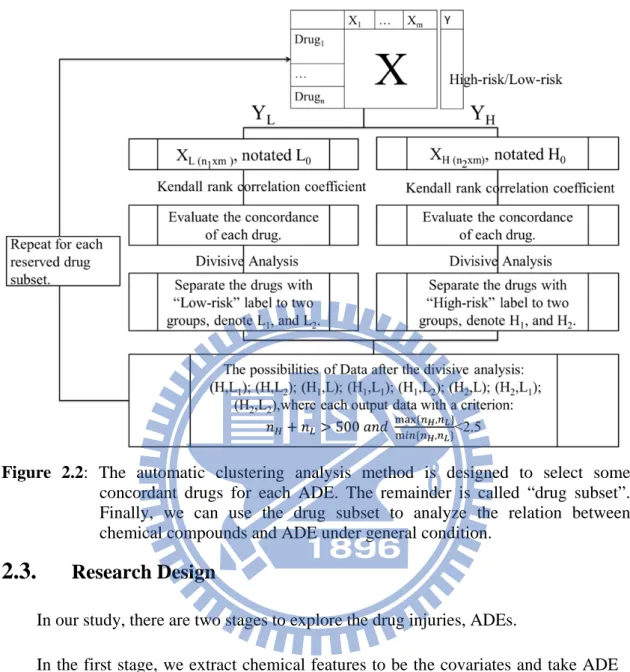
Find concordant drug subset determined by ADE risk-index and chemical features

We build an automatic work flow to find concordant drug subset for each ADE. The

drug subset contains two types of ADE risk-index (high-risk or low-risk). For drugs in

each type, they are more similar in drugs’ chemical feature set.

The workflow is described as the following, and Figure 2.2 shows the flow chart of

it:

(1)

Given an ADE, we separate the drug set into two groups (Notation:

,

),

one is collected low-risk drugs ( ), and the other group is collected high-risk

drugs ( ).

(2)

Use Kendall rank correlation coefficient to evaluate the concordance between

each two drugs on feature space.

―

For

group with

high-risk drugs, we build an

Kendall

table notated as

TABLE

:

TABLE

―

For

group with

high-risk drugs, we build an

Kendall

table notated as

TABLE

.

(3)

Use divisive analysis to divide items into two clusters.

― For

group, we take the

1

TABLE

as a distance matrix. Then,

we divide

items into two clusters (Notation:

and ).

― For

group, we take the

1

TABLE

as a distance matrix. Then,

we divide

items into two clusters (Notation:

and ).

(4)

We consider these eight possibilities of drug subset:

,

,

,

,

,

,

,

,

,

,

,

,

,

,

,

(5)

If the drug subset,

,

,

,

0, 1, 2, satisfy the number of drugs lager

than 500 and

#

,#

#

,#

2.5,

then the drug subset

,

is the possibility of concordant drug subset. We

take this drug subset as

,

and repeat the steps from (1) to (4).

Figure 2.2: The automatic clustering analysis method is designed to select some

concordant drugs for each ADE. The remainder is called “drug subset”.

Finally, we can use the drug subset to analyze the relation between

chemical compounds and ADE under general condition.

2.3.

Research Design

In our study, there are two stages to explore the drug injuries, ADEs.

In the first stage, we extract chemical features to be the covariates and take ADE

record to be the drugs’ risk-index as the response variable. C4.5 Decision tree is used to

obtain the mapping function from chemical feature space onto the binary risk-index

space. Then, we use 10-fold cross-validation to estimate the prediction model accuracy.

The resulted decision tree is the build ADE prediction model with associated chemical

features. The ADE prediction models on the first stage are called Initial Decision Trees

(IDTs). It serves as feature selection for each ADE. We use “rpart” package of

statistical software R to obtain the IDTs for each ADE. Finally we compare the

prediction accuracy among three chemical feature sets for each ADE. The aim of the

first stage is to compare the performance of different chemical feature sets and obtain

the associated chemical features for each ADE.

The performance of IDT implies that there exists an instance subset that is

relatively more separable in the associated feature space. We call this instance subset as

concordant drug subset. It is illustrated in Figure 2.3.

Figure 2.3: This figure illustrates the concordant drug subset is red-surrounded. The

triangle and circle drugs are shown for binary ADE risk index.

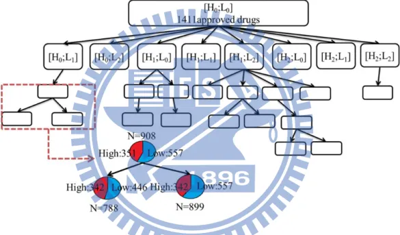
In the second stage, we develop an automatic analysis work flow to obtain

concordant drug subset on each ADE of interest. After divisive clustering, we can get

several drug subsets which are candidate concordant drug subsets of a particular ADE.

Finally, we take the drug subset as the data set and use 10-fold CV and decision tree to

build a set of candidate models for the fixed ADE. Among all of candidate models, we

choose the optimal model with the highest prediction accuracy. For instance, we have

29 drug subsets as illustrated in Figure 2.3. The 29 drug subset is obtained by divisive

clustering analysis. Each node stands for a drug set with binary risk index. The high risk

the low risk drugs. There can be 8 children of each node at most due to the combination

illustrated in the first level in Figure 2.3. Among 29 drug subset, each has a candidate

model and each model represents a decision tree with its own 10-fold CV accuracy. The

model with the highest 10-fold CV accuracy is the final ADE prediction model. The

optimal prediction models of ADEs are called “Similarity Guided Decision Tree”

(SGDT). Figure 2.4 gives an overall view of our research.

Figure 2.4: For an ADE, we have an initial drug set and use automatic clustering analysis

to get numerous drug subsets which contain concordant drugs. Put the initial

drug set into automatic clustering analysis, then we can get several drug

subsets which satisfy the condition we set. Each drug subset could be another

initial drug set in the next level, and iteratively execute the automatic

clustering analysis. The iteration stops until none of output file satisfies the

criteria we set.

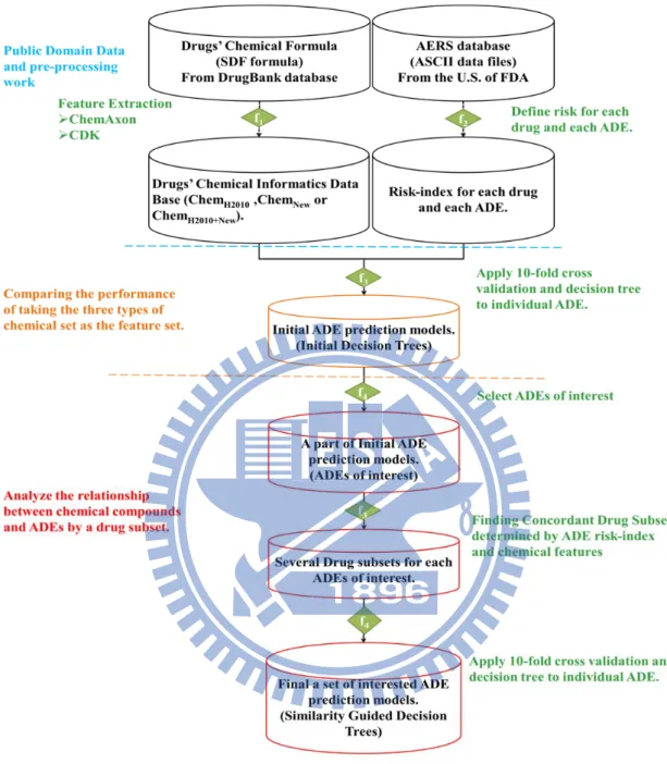
Figure 2.5: The flow chart of our research. The first step is material collection and

pre-processing work. The pre-processing work is to get the risk-index for

each drug and each ADE. The second step is to compare the performance

of ADE prediction models which generate by taking three types of

chemical sets as the feature set, such as, Chem

, Chem

, and

Chem

. The most important of our research is the part which

locates below the orange dashed line. This step is to analyze the relation

between chemical compounds and ADEs of interest under some regular

3. Results

The most important of our research is that we build an automatic concordant

analytic method. We use automatic clustering analysis, 10-fold cross-validation and

decision tree to analyze the relation between chemical compounds and ADEs under some

regular condition. We define the prediction accuracy and the ratio of

to

evaluate the performance of ADE prediction.

3.1. Compare the performance by using different types of chemical

feature sets.

There are three issues to compare the performance of prediction model by using

three different types of chemical feature sets,

,

, and

:

Q 1.

Can we find some ADEs (

∗′

s), satisfying X

→

∗

, with a

good prediction function?

Q 2.

Given those

∗′

s, can we verify if the performance of X

→

∗

_{is better than that of X}

_→

∗

_?

Q 3.

If we get the negative answer in Q 2, can we verify if the performance of

X

→

∗

_{is better than that of}

_X

_→

∗

_?

In the first question, we define some criterion to judge the performance of ADE

prediction models. Let the upper bound of 95% C.I. of

be the threshold. If

of an ADE model is larger than the threshold, then we consider this

ADE model as an acceptable prediction model. We find 642 out of 1,483 ADEs that has

the prediction accuracy higher than the threshold, shown in Figure 3.1(a). Considering

the second question, we can find 121 ADEs whose prediction accuracy of using

Chem

as the feature set is higher than using Chem

, shown in Figure 3.1(b). For

answering the third question, we use 841 ADEs which have negative response in the

second question. Then, we test whether the prediction accuracy of using Chem

as the feature set is higher than using Chem

. The result shows that there are only 44

ADEs which indicate that the prediction accuracy of using Chem

is better

than using Chem

, shown in Figure 3.1(c).

Figure 3.1(a): Each red point denotes that the ADE model’s

is higher than the

threshold. And each blue point denotes that the ADE model’s

is not higher than the threshold.

0.50 0.55 0.60 0.65 0.70 0 .45 0. 5 0 0. 5 5 0. 60 0. 65 0 .70

(a) Question1:Cut Value:0.9712839

Random Guess

P

re

di

ct

ion

A

c

c

ur

ac

y

w

it

h

Ch

em

.(

H

20

10

)

Figure 3.1(b): In the scatter plot, the red points (121 points) denote that the performance

of using the

feature set to build an ADE model is better than

using the

feature set. The blue points denoted that the

performance of using the

feature set to build model is not

better than using

.

Figure 3.1(c): Among 841 ADEs have a negative answer in Q 2; there are only 44 ADEs

(red points) which satisfy that the performance of using

is better than using

.

0.50 0.55 0.60 0.65 0.70 0. 45 0. 50 0. 5 5 0. 60 0. 65 0 .70

(b) Question2

Prediction Accuracy with Chem(H2010)

P

red

ic

ti

on A

c

c

u

ra

c

y

w

ith C

h

em(

N

e

w

)

(c) Question3

Prediction Accuracy with Chem(H2010)

Pr

edi

c

ti

on

Ac

c

ur

ac

y

w

it

h C

he

m

(H

20

10+N

ew

)

After comparing the performance of using different types chemical feature sets, we

find that no matter which feature set we take to build ADE models, the prediction

accuracy of each ADE is not higher than 0.8. The accuracy rate will decrease rapidly if

we consider multiple ADEs. For illustration, suppose we are interested in a new drug is

high-risk or low-risk drug corresponding to 3 specific ADEs and of each ADEs, the

prediction rate is 0.8. Then the total prediction accuracy would be reduced to 0.8

0.512. Therefore, we need to increase the prediction accuracy of ADE models as higher

as possible.

3.2. Select concordant drugs and then analyze the relation between

chemical compounds and ADE under some regular condition

We build an automatic concordant analysis to select concordant drugs. Then, we

take the remaining drugs as data set to build prediction models by decision tree. Finally,

we use 10-fold cross-validation to estimate the prediction accuracy of each ADE model.

3.2.1. ADEs of interest filtering.

In order to check the feasibility of this automatic concordant analysis, we need to

construct testing data. There are a lot of ADEs in our study (1,483 ADEs), so we select

some ADEs to be the testing data. In this thesis, we filter out the ADE of interest by

considering the 10-fold CV accuracy to the guess rate:

.

We use the ADEs’ prediction accuracy as the response variable and the guess rate as the

covariate to build a simple linear regression, where the prediction accuracy is generated

by taking

Chem

as the feature set and the prediction model is called “Initial

Decision Tree” (IDT). If the accuracy of an ADE model is higher than the upper bound of

95% prediction interval of accuracy, then the ADE is one of the “ADEs of interest”.

Among 1,384 ADEs, we obtain 35 ADEs which satisfy that the accuracy is higher than

the upper bound.

Now we use these ADEs of interest to analyze the relationship between drugs’

chemical compounds and ADEs under some regular condition. These prediction models

are called “Similarity Guided Decision Tree” (SGDT). In Figure 3.2 (a), we compare the

prediction accuracy between IDT (blue bars) and SGDT (red bars) for each “ADEs of

interest”, where the drug subset contains the remaining drugs after doing automatic

clustering analysis. Obviously, the prediction accuracy of SGDT is higher than IDT for

each ADEs of interest.

What we are most interested in is the ratio between prediction accuracy and guess

rate, for the guess rate has a significant effect on the prediction accuracy. The high

random guess shows that the majority of drugs belong to one kind of drug-risk level

(high-risk or low-risk). As a result, we just guess all of drugs are belong to this drug-risk

level, and then the prediction accuracy rate is naturally high. In order to avoid this

situation, we need to consider the ratio,

. The higher ratio illustrates

that the prediction model is more reliable. In Figure 3.2(b), we compare the ratio,

between IDT and SGDT for each ADEs of interest. Since the red bar

(SGDT) is higher than the blue bar (IDT) of each interest ADEs. Consequently, we

conclude that the performance of using an appropriate drug subset is better than using a

fixed drug set for these ADEs of interest.

Figure 3.2(a): In this bar plot, each red bar denotes that the performance of an ADE

prediction model after doing the automatic clustering analysis, and each

blue bar denotes the performance of ADE model by using initial drug set.

Figure 3.2(b): For each ADEs of interest, the ratio,

by using a drug

subset (red bar) is higher than using a fixed drug set (blue bar).

In summary, the results of interested ADEs’ prediction models show that 24 ADEs

have the prediction accuracy greater than 80%. However, if we consider the ratio

between prediction accuracy and guess rate, we can find 33 ADEs of interest have

1.3 among 35 ADEs of interest.

Among these 35 ADEs of interest, there are three more serious ADEs: Diabetes

Mellitus (PT

), Renal Failure Acute (PT

) and Renal Impairment (PT

).

(1)

DIABETES MELLITUS (PT

):

Feature Set:

Drug Size: 1,411 approval drugs

By automatic clustering analysis (the second stage), the prediction accuracy is

listed as following:

IDT

0.0085

524

538

1062

0.493

0.527

SGDT

489

244

733

0.667

0.871

Figure 3.3: The SGDT of the ADE-DIABETES MELLITUS for 489 high-risk drugs and

244 low-risk drugs (

733), with a prediction accuracy of 0.871.

Table 3.1: The chemical description of features we used in the ADE model.

Feature Code Feature Name

Parameter/

Discriptive Statistic

X1_0_113_2

JCStericEffectIndex

Atom=false

X1_0_75_1

JCMinimalProjectionArea

None

X1_0_77_1

JCMinZ

None

X2_0_41_1

JAR_hmoelectrophiliclocaliz

ationenergy_Localization

energy L(+)

IQR

X2_0_81_1

JAR_sterichindrance

None

X2_0_90_1

JAR_wienerpolarity

None

X3_0_2_1

SDF_ALOGPS_LOGS

None

Table 3.1 (Continue)

(2)

RENAL FAILURE ACUTE (PT

)

Feature Set:

Drug Size: 1,411 approval drugs

By divisive analysis (the second stage), the prediction accuracy is listed as

following:

Cut

Value High Low N

Guess

Rate

Accuracy

IDT

0.027

539

438

977

0.552

0.531

SGDT

508

231

739

0.687

0.910

Feature Code Descriptor

Definition

X1_0_113_2

JCStericEffectIndex

Steric effect index

X1_0_75_1

JCMinimalProjectionArea Calculates the minimal projection area

X1_0_77_1

JCMinZ

Returns the minimum z coordinate

of the bounding box.

X2_0_41_1

JAR_hmoelectrophilicloc-alizationenergy

HMO Electrophilic localization energy L(+).

X2_0_81_1

JAR_sterichindrance

Steric hindrance

X2_0_90_1

JAR_wienerpolarity

Wiener polarity

X3_0_2_1

SDF_ALOGPS_LOGS

"The extent to which a compound will

dissolve in water. The log of solubility is

generally inversely related to molecular

weight."- U.S. Environmental Protection

Agency, 2009

Figure 3.4: The SGDT of the ADE- RENAL FAILURE ACUTE for 508 high-risk drugs

and 231 low-risk drugs (

739), with a prediction accuracy of 0.910.

Table 3.2 (Continue)

(3)

RENAL IMPAIRMENT (PT

)

Feature Set:

Drug Size: 1,411 approval drugs

By divisive analysis (the second stage), the prediction accuracy is listed as

following:

Cut Value

High

Low

N

Guess Rate

Accuracy

IDT

0.006

561

548

1109

0.506

0.526

SGDT

247

257

504

0.510

0.946

Feature Code

Descriptor

Definition

X2_0_21_29

JAR_composition

Elemental composition calculation (w/w%).

X2_0_39_9

JAR_hmoelectro-ndensity

HMO Electron density.

X2_0_44_1

JAR_hmolocalizat-ionenergy

HMO Electrophilic localization energy L(+).

X2_0_52_6

JAR_localization-energy

Localization energy L(+)/L(-).

X2_0_57_1

JAR_msacc

Hydrogen bond acceptor average

multiplicity over microspecies by pH.

X2_1_8_1

JAR_aromatic-bondcount

Aromatic bond count.

X4_0_29_7

RCDK_KierHall-SmartsDescriptor

A fragment count descriptor

that uses e-state fragments

X4_1_20_6

RCDK_CPSA-Descriptor

Calculates 29 Charged Partial Surface Area

(CPSA) descriptors. One of them is FNSA.3.

FNSA.3=the ratio between charge weighted partial

negative surface area and total molecular surface area.

Figure 3.5: The SGDT of the ADE- Renal Impairment for 247 high-risk drugs and 257

low-risk drugs (N=504), with a prediction accuracy of 0.946.

Table 3.3: The description of features we used in the ADE model.

Feature Code

Feature Name

Parameter/

Discriptive Statistic

Descriptor

Definition

X4_0_19_9

RCDK_VP.0

None

RCDK_ChiPathDescriptor

Evaluates chi path

4. Discussion and Conclusions

4.1. Discussion

In our research, we find that the size of drug subset is smaller for each ADEs after

conducting automatic concordant analysis. Therefore, we do some check-up on these

“unselected drugs”.

Given an ADE, we can examine the Kendall τ rank correlation coefficient

between “unselected drugs” and “selected drugs” in the chemical feature space. For each

“unselected drug”, we choose a most similar “selected drug” which has the maximum τ

value. Then, we compare the corresponding risk-indices.

If the risk-indices are different between some unselected drug and some most similar

selected drug, the unselected drug is called “mislabel” drug. Otherwise, if the drug-risk of

some unselected drug and some most similar selected drug are the same, the unselected

drug is called “concordant” drug. For example, we can get results for Renal Failure Acute

and Diabetes Mellitus as the following table:

Table 4.1 Show the number of unselected drugs and selected drugs for the two

ADEs of interest.

We list out the possible speculations for mislabel and concordant as the following:

(1)

Mislabel:

Mislabel drugs can be separated into two cases:

(1.1) The unselected drug is a low-risk drug, and the most similar selected

drug is a high-risk drug. There are several possible reasons of this case:

(1.1.1) The drug is used for particular patients. The patient population

(1.1.2.1) AERS does not cover all adverse event occurrences

globally.

(1.1.2.2) The newly marketing drugs documented in shorter history

tend to have less observation.

(1.2) The other case is that the unselected drug is a high-risk drug, and the

most similar selected drug is a low-risk drug. The possible reason of this

case is that the drug may be a concomitant drug, such as, second suspect

drug, concomitant drug, and interacting drug. This kind of drugs tends

to have higher reports.

For example, in Renal Failure Acute prediction model, the approval history duration

of the two low-risk drugs (DB01193, DB00488) are at least less than ten years comparing

to the most similar selected drugs (DB00190, DB01168). Therefore, the observed ADE

report frequency may lead us to underestimate their risk propensity.

Table4.2 Show the approval date of the two unselected drugs and two “the most

similar” selected drugs.

(2)

Concordant

Given an ADE risk-index (high or low), some unselected drugs are actually

relatively closer to the selected drug group. For instance, drug A, drug B and

other four drugs are the same ADE risk-indexed. However, drug A and drug B

are determined as unselected by our automatic analysis method. As shown in

Figure 4.1, drug B are actually closer to the four selected drugs.

Unselected Drug Approval date Risk-index

Most similar

selected drug

Approval date

Risk Index

DB01193

1999/12/30

Low-risk

DB00190

Approved Prior to

jan 1, 1982

High-risk

DB00488

1990/12/26

Low-risk

DB01168

Approved Prior to

Figure 4.1: (a) The first division separates drug A from the other five drugs. (b) The

second division separates drug B from the other four drugs. (c) The

remained four drugs are determined as selected drugs. Drug A is relatively

far from the four selected drugs in chemical feature space, while drug B is

relatively closer to the four selected drugs.

4.2. Conclusion

In our research, we identify 1,384 ADEs with corresponding associated chemistry

informatics features by decision tree. With an automatic analysis work flow, we can

obtain a concordant drug subset with satisfying 10-fold cross-validation accuracy. The

test experiment about selected 35 ADEs of interest results in accuracy higher than 80%.

Three observations from the results are worth emphasizing:

(1)

After conducting the automatic analytic method, these drugs give a significant

drug-risk level. This leads to significant results of decision tree.

(2)

Compared with the research of Hammann et al., we consider more ADEs,

chemical features and approval drugs to build a set of ADE prediction models.

(3)

There are 35 ADE models with the prediction accuracy higher than 0.8.

The practical benefits of our experimental results are of great interest both for the

R&D in medicine industry and in public health. We can apply the trained model to

forecast the new designed drugs (potential compounds) for its ADE. In addition, we can

recognize the probability of some ADE occurrence when some chemical compound exits.

Our models can not only guide future clinical trials, but also run monitoring and test

during such trials. Moreover, they allow pharmacists for more advanced and efficient

drug design.

4.3. Recommendation for Future Research

Our analysis is focused on the relation between chemical compounds and ADEs. In

fact, the process of drug-related injuries resulted in some adverse reaction is still a “black

box”. After years of study, many experts believe that the types of elements which result

in drug-related injuries are not only chemical compounds, but also target gene. Some

scholars have proposed some other view about the causes of adverse reactions (Berger,

2011). In their approach, they believe that drug side effect is mediated by complex

cellular networks. In response to a drug, the variations in cellular networks can expose

silent phenotypes. This type of adverse drug event is caused by inheritance. Namely, if

we only use chemistry features, we cannot thoroughly explain this type of adverse drug

events.

In the future studies, to break the limitation of ADEs’ study, we can consider other

factors which may result in drug-related injuries, such as, drugs’ target gene and ADME

mechanism. Thus, it may be of interest for future research that we combine the systems

biology and drugs' chemistry to build ADE prediction model. The ADE models not only

have higher prediction accuracy but also contain more "selected drugs". That means the

"concordant drug" are really dissimilar to a "selected drug" on the "new" feature space

(combine chemistry and system biology), where the two drugs have the same risk-index.

Reference:

[1] Ritter, J. M. (2008). Minimising Harm: Human Variation and Adverse Drug

Reactions (ADRs). British Journal of Clinical Pharmacology.

[2] Berger, S. I., and Iyengar R. (2011). Role of systems pharmacology in understanding

drug adverse events. WIREs Systems Biology and Medicine.

[3] Hammann, F., and Gutmann, H. (2010). Prediction of Adverse Drug Reactions

Using Decision Tree Modeling. Clinical Pharmacology & Therapeutics, 88 (1), 52–

59.

[4] U.S. Food and Drug Administration. (2012). Adverse Event Reporting System

(AERS). Retrieved July 01, 2011, from http://www.fda.gov/Drugs/default.htm

[5] Departments of Computing Science & Biological Sciences, University of Alberta.

(2012). DrugBank. Retrieved July 5, 2011, from http://www.drugbank.ca/

[6] Marvin was used for drawing, displaying and characterizing chemical structures,

substructures and reactions, Marvin 5.9.3 (version number), 201n (insert year of

version release), ChemAxon (http://www.chemaxon.com)

[7] Guha, R. (2007). 'Chemical Informatics Functionality in R'. Journal of Statistical

Software 6(18)

[8] Michael J. A. (1997). Data Mining Techniques. New York: WILEY

[9] Wasserman, L. (2004). All of statistics a concise course in statistical inference. New

York: Springer.

[10] Keiser M. J., and Setola V. (2009). Predicting new molecular targets for known

drugs. Nature, 462:175–181.

[11] Campillos M., and Kuhn M. (2008). Drug target identification using side-effect

similarity. Science, 321:263–266.

[12] Pouliot, Y., and Chiang, A.P. (2011). Predicting Adverse Drug Reactions Using

Publicly Available PubChem BioAssay Data. Nature, 90(1):90-99.

[13] Huang, L.C., and Wu, X. (2011). Predicting adverse side effects of drugs.  BMC

Genomics

No. Feature Name Chemcial Descriptors #ofNA Source v5.1Code 1 JCChainAtomCount JCChainAtomCount 0 ChemAxonByExcel 1_1_27_1 2 JCCarboRingCount JCCarboRingCount 0 ChemAxonByExcel 1_1_25_1 3 JClogP JClogP 0 ChemAxonByExcel 1_1_68_1 4 JCFusedAromaticRingCount JCFusedAromaticRingCount 0 ChemAxonByExcel 1_1_50_1 5 JCFusedRingCount JCFusedRingCount 0 ChemAxonByExcel 1_0_51_1 6 JClogD(9) JClogD 0 ChemAxonByExcel 1_1_67_5 7 JClogD(5) JClogD 0 ChemAxonByExcel 1_1_67_3 8 JCChainBondCount JCChainBondCount 0 ChemAxonByExcel 1_1_28_1 9 JCIsoelectricPoint JCIsoelectricPoint 0 ChemAxonByExcel 1_0_60_1 10 JCSmallestRingSize JCSmallestRingSize 0 ChemAxonByExcel 1_1_111_1 11 JCBalabanIndex JCBalabanIndex 0 ChemAxonByExcel 1_1_19_1 12 JClogD(11) JClogD 0 ChemAxonByExcel 1_1_67_2 13 JCDonorCount JCDonorCount 0 ChemAxonByExcel 1_1_41_1 14 JCResonantCount JCResonantCount 2 ChemAxonByExcel 1_1_100_1 15 JCAcceptorSiteCount JCAcceptorSiteCount 0 ChemAxonByExcel 1_1_3_1 16 JCAromaticAtomCount JCAromaticAtomCount 0 ChemAxonByExcel 1_1_12_1 17 JCBasicpKa(strongness=1) JCBasicpKa 87 ChemAxonByExcel 1_1_20_1 18 JCBasicpKa(strongness=2) JCBasicpKa 292 ChemAxonByExcel 1_1_20_2 19 JCAcidicpKa(strongness=1) JCAcidicpKa 306 ChemAxonByExcel 1_1_4_1 20 JCAcidicpKa(strongness=2) JCAcidicpKa 732 ChemAxonByExcel 1_1_4_2 21 JCRingCount JCRingCount 0 ChemAxonByExcel 1_1_104_1 22 JCAliphaticBondCount JCAliphaticBondCount 0 ChemAxonByExcel 1_1_7_1 23 JClogD(7.4) JClogD 0 ChemAxonByExcel 1_1_67_4 24 JCDonorSiteCount JCDonorSiteCount 0 ChemAxonByExcel 1_1_42_1 25 JCPSA(PH=12) JCPSA 0 ChemAxonByExcel 1_0_83_1 26 JCQ_N JCQ_N 0 ChemAxonByExcel 1_1_93_1 27 JCQ_O JCQ_O 0 ChemAxonByExcel 1_1_95_1 28 JCQ_C JCQ_C 0 ChemAxonByExcel 1_1_87_1 29 JCQ_halogen JCQ_halogen 0 ChemAxonByExcel 1_1_90_1 30 JCQ_azole JCQ_azole 0 ChemAxonByExcel 1_1_85_1 31 JCQ_phenol JCQ_phenol 0 ChemAxonByExcel 1_1_96_1 32 JCQ_ketone JCQ_ketone 0 ChemAxonByExcel 1_1_91_1 33 JCQ_amine JCQ_amine 0 ChemAxonByExcel 1_1_84_1 34 JCQ_COOH JCQ_COOH 0 ChemAxonByExcel 1_1_88_1 35 JCQ_benzene JCQ_benzene 0 ChemAxonByExcel 1_1_86_1 36 JCQ_ester JCQ_ester 0 ChemAxonByExcel 1_1_89_1 37 JCQ_nitro JCQ_nitro 0 ChemAxonByExcel 1_1_94_1 38 JCQ_methyl JCQ_methyl 0 ChemAxonByExcel 1_1_92_1 39 JCQ_S JCQ_S 0 ChemAxonByExcel 1_0_97_1 40 JCAcceptorCount JCAcceptorCount 0 ChemAxonByExcel 1_0_2_1 41 JClogD(0) JClogD 4 ChemAxonByExcel 1_1_67_1 42 JCMolecularPolarizability JCMolecularPolarizability 4 ChemAxonByExcel 1_0_78_1 43 JCAliphaticAtomCount JCAliphaticAtomCount 0 ChemAxonByExcel 1_1_6_1 44 JCBondCount JCBondCount 0 ChemAxonByExcel 1_1_23_1 45 JCFusedAliphaticRingCount JCFusedAliphaticRingCount 0 ChemAxonByExcel 1_1_49_1 46 JCHeteroRingCount JCHeteroRingCount 0 ChemAxonByExcel 1_1_58_1 47 JCHyperWienerIndex JCHyperWienerIndex 0 ChemAxonByExcel 1_1_59_1 48 JCRandicIndex JCRandicIndex 0 ChemAxonByExcel 1_1_98_1 49 JCAcceptor(PH=0) JCAcceptor 0 ChemAxonByExcel 1_0_1_1 50 JCAcceptor(PH=1) JCAcceptor 4 ChemAxonByExcel 1_0_1_2 51 JCAcceptor(PH=2) JCAcceptor 9 ChemAxonByExcel 1_0_1_8 52 JCAcceptor(PH=3) JCAcceptor 10 ChemAxonByExcel 1_0_1_9 53 JCAcceptor(PH=4) JCAcceptor 10 ChemAxonByExcel 1_0_1_10 54 JCAcceptor(PH=5) JCAcceptor 11 ChemAxonByExcel 1_0_1_11 55 JCAcceptor(PH=6) JCAcceptor 13 ChemAxonByExcel 1_0_1_12 56 JCAcceptor(PH=7) JCAcceptor 13 ChemAxonByExcel 1_0_1_13 57 JCAcceptor(PH=8) JCAcceptor 15 ChemAxonByExcel 1_0_1_14 58 JCAcceptor(PH=9) JCAcceptor 18 ChemAxonByExcel 1_0_1_15 59 JCAcceptor(PH=10) JCAcceptor 23 ChemAxonByExcel 1_0_1_3 60 JCAcceptor(PH=11) JCAcceptor 27 ChemAxonByExcel 1_0_1_4 61 JCAcceptor(PH=12) JCAcceptor 33 ChemAxonByExcel 1_0_1_5 62 JCAcceptor(PH=13) JCAcceptor 39 ChemAxonByExcel 1_0_1_6 63 JCAcceptor(PH=14) JCAcceptor 48 ChemAxonByExcel 1_0_1_7 64 JCAcidicpKaLargeModel(strongness=1) JCAcidicpKaLargeModel 303 ChemAxonByExcel 1_0_5_1 65 JCAcidicpKaLargeModel(strongness=2) JCAcidicpKaLargeModel 723 ChemAxonByExcel 1_0_5_2 66 JCAcidicpKaLargeModel(strongness=3) JCAcidicpKaLargeModel 1006 ChemAxonByExcel 1_0_5_3 67 JCAcidicpKaLargeModel(strongness=4) JCAcidicpKaLargeModel 1150 ChemAxonByExcel 1_0_5_4 68 JCAcidicpKaLargeModel(strongness=5) JCAcidicpKaLargeModel 1209 ChemAxonByExcel 1_0_5_5 69 JCAcidicpKaLargeModel(strongness=6) JCAcidicpKaLargeModel 1222 ChemAxonByExcel 1_0_5_6 70 JCAcidicpKaLargeModel(strongness=7) JCAcidicpKaLargeModel 1224 ChemAxonByExcel 1_0_5_7 71 JCAcidicpKaLargeModel(strongness=8) JCAcidicpKaLargeModel 1226 ChemAxonByExcel 1_0_5_8 72 JCAliphaticRingCount JCAliphaticRingCount 0 ChemAxonByExcel 1_0_8_1