盲蔽式非同調頻譜偵測之研究

國 立 交 通 大 學

電信工程學系

碩 士 論 文

盲蔽式非同調頻譜感測之研究

On Blind Non-coherent Spectrum Sensing

研 究 生：蘇郁文

指導教授：蘇育德 博士

盲蔽式非同調頻譜感測之研究

On Blind Non-coherent Spectrum Sensing

研 究 生：蘇郁文

Student : Yu-Wen Su

指導教授：蘇育德

Advisor : Yu T. Su

國 立 交 通 大 學

電 信 工 程 學 系 碩 士 班

碩 士 論 文

A Thesis Submitted to

The Department of Communications Engineering

College of Electrical and Computer Engineering

National Chiao Tung University

In partial Fulfillment of the Requirements

For the Degree of Master of Science

In

Communications Engineering

July 2008

Hsinchu, Taiwan, Republic of China

中 華 民 國 九 十 七 年 七 月

盲蔽式非同調頻譜感測之研究

研究生︰蘇郁文 指導教援︰蘇育德 博士

國立交通大學

電信工程系碩士班

中文摘要

傳統的頻譜政策，每個特定的頻帶僅允許其主要使用者(註冊有該

頻帶的使用執照)使用，其他未註冊的使用者皆被禁止使用。然而，

在頻譜需求日益成長的今天，新的感知網路概念被提出來︰在不干擾

主要使用者的前提之下，允許其他使用者使用閒置中的頻帶，期望制

定一個良好的自我管理規範，能夠有效地提高頻譜使用率。

為了實現感知網路，快而準確的頻譜偵測為最基本的功能需求，

而傳統所使用的偵測方法在雜訊能量不確定的情況下，效能將受到嚴

重的損失。在本文中，考慮單通道與多通道，我們提出二種能適用於

各種不同感知網路運用的頻譜偵測演算法，在訊號能量、型態、通道

頻率響應、甚至雜訊能量皆未知的情況下都能成功達成偵測。根據模

擬的結果，在 IEEE 802.22 的規格標準下，我們所提出的演算法，可

以確實避免雜訊能量的不確定性對偵測結果所帶來的影響。

On Blind Non-coherent Spectrum Sensing

Student: Yu-Wen Su Advisor: Yu T. Su

Department of Communications Engineering National Chiao Tung University

abstract

The conventional spectrum policy allows only primary users (licensee) the exclusive right to access the allocated band while other users (secondary users) are prohibited from using the same band. Cognitive radio (CR) represents a paradigm shift that would permit a secondary user to access the licensed band whenever it is not used (by primary users). Ideally, the CR paradigm envisions a autonomous, self-regulated spectrum usage scenario that makes any regulation agencies whence spectrum licenses completely obso-lete. Before this spectrum utopia is realized, however, we have to settle for and make the most of the transitional but feasible coexistence-with-access-priority scenario.

To implement any CR network, a fundamental functional requirement is the avail-ability of a multitude of fast and accurate spectrum sensing techniques. Conventional radiometers (i.e., energy detector) or radiometer array offers outstanding sensing per-formance when the noise level is perfectly known. However, they suffers from serious degradation when there is a noise level uncertainty. This thesis proposes various robust spectrum sensing algorithms which requires little or no information about the sensed channel or/and the primary signal structure. Both single-channel and multiple-channel scenarios are considered. Computer simulations are performed to evaluate and com-pare the sensing performance of the proposed algorithms. Numerical results show that our algorithms do provide satisfactory performance which is insensitive to noise level uncertainty.

Contents

Abstract i

Contents ii

List of Figures iv

List of Tables viii

1 Introduction 1

2 Spectrum sensing algorithm 3

2.1 Neyman Pearson Criterion . . . 4

2.2 Energy detector [4] . . . 5

2.3 Signal of digital television [6] . . . 6

2.4 SUI channel model . . . 10

3 Multi-tone Detector 13 3.1 System model of multi-tone detector . . . 13

3.2 The FCME algorithm . . . 14

3.3 The FBCME algorithm . . . 19

4 Single-tone Detector 23 4.1 Eigenvalue based sensing algorithms . . . 23

4.3 Modified Ratio Detector . . . 30

5 Joint estimation and detection 35

5.1 Moment estimation . . . 35

5.2 Momnet estimation in Likelyhood ratio test . . . 40

6 Conclusion 44

List of Figures

2.1 Pulse shaping of signal pass VSB filter. . . 4

2.2 Energy detector. . . 5

2.3 Passband VSB system. . . 7

2.4 Square root raise cosine pulse shaping. . . 9

2.5 Pulse shaping of signal pass VSB filter. The left one is real part signal and the right one is the imaginary part signal. . . 9

2.6 Pulse shaping of signal pass VSB filter. . . 9

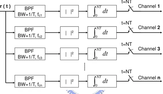
3.1 Energy detector array for multi-tone detector. . . 14

3.2 Energy detector output for multi-tone detector. The output of channels with signal would be accumulated with larger power than which of signal free channels. It can justify easily that channels with larger outputs would have signal existed. . . 15

3.3 Deflection coefficient of T=yi+1 P yi, N = 10, λ = 10 (SN R = 0dB). . . 17

3.4 Detection probability of FCME algorithm with different initial clean set. Simulation with QPSK signal passing by SUI3 fading channel in 20 dif-ferent frequency bands. The prior probability of signal existing or not is 50%. . . 18

3.6 Detection Probability of FBCME algorithm. Simulation with DTV signal passed by SUI3 fading channel in 20 different frequency bands. The prior probability of signal existing or not is 50%. The optimal energy detector

means that energy detector without noise uncertainty. . . 21

3.7 Detection probability of FBCME algorithm suffered by noise uncertainty. Simulation with DTV signal passed by SUI3 fading channel in 20 different

frequency bands. The prior probability of signal existing or not is 50%. . 22

3.8 False alarm probability of FBCME algorithm suffered by noise uncer-tainty. Simulation with DTV signal passed by SUI3 fading channel in 20 different frequency bands. The prior probability of signal existing or not

is 50%. . . 22

4.1 Mathematical model of a real time autocorrelation detector.[3] . . . 25

4.2 Mathematical model of energy detector output through a power sampler

processer. . . 27

4.3 Mathematical model of ratio detector. . . 28

4.4 Detection probability of ratio detector. Simulation with QPSK signal

passing through SUI3 fading channel. . . 29

4.5 False alarm probability of ratio detector. Simulation with QPSK signal

passing through SUI3 fading channel. . . 29

4.6 Probability density function of noncentral F distribution. The left figure is noncentral F distribution with the same degrees of freedom and differ-ent noncdiffer-entral parameter. The right one is F distribution with differdiffer-ent

degrees of freedom. . . 30

4.7 Mathematical model of ratio detector.where P [n] is a random sequence with element {1,-1}, each element has equal probability. . . 31

4.8 Detection probability of modified ratio detector. Simulation by QPSK

4.9 False alarm probability of modified ratio detector. Simulation by QPSK

signal passing through SUI3 fading channel. . . 32

4.10 Detection probability of modified ratio detector. Simulation by DTV signal passing through SUI3 fading channel. The highly correlation of

signal would rise the detection performance significantly. . . 33

4.11 False alarm probability of modified ratio detector. Simulation by DTV

signal passing through SUI3 fading channel. . . 33

5.1 System model of equivlent energy detector. . . 35

5.2 Error ratio of estimated noise variance in H1 case, AWGN. . . 37

5.3 Histogram for error ratio of estimated noise variance σ2 _{in H1 case,}

AWGN. The estimation error would cause about 5% noise uncertainty. . 38

5.4 Histogram for error ratio of estimated noise variance σ2 _{in H0 case,}

AWGN. The left tail of histogram is caused by equation 5.4 that ˆσ2 ₌

ˆ

E − p ˆE2_{− ˆvar, when E converge to σ}2 _{faster than s}2 ₌ p ˆ_E2_{− ˆvar}

converge to 0, the estimated noise power σ2 _{would be smaller than exact}

value. . . 38

5.5 Detection probability of energy detector using moment estimation in AWGN.

N=100000, m1=10, m2=10000, the estimation error is about 1dB noise

uncertainty. . . 39

5.6 False alarm probability of energy detector using moment estimation in

AWGN. N=TW=100000, m1=10, m2=10000 . . . 39

5.7 Histogram for ˆA for H1 case. . . 41

5.8 Histogram for ˆσ2

1 for H1 case. . . 41

5.9 Histogram for ˆσ2

0 for H1 case. . . 41

5.10 Histogram for ˆA for H0 case. . . 42

5.11 Histogram for ˆσ2

1 for H0 case. . . 42

5.12 Histogram for ˆσ2

5.13 Detection probability of Likelyhood ratio test and energy detector without noise uncertainty, simulation with QPSK signal passing through AWGN

channel, TW=100. . . 43

5.14 False alarm probability of Likelyhood ratio test and energy detector with-out noise uncertainty, simulation with QPSK signal passing through AWGN

List of Tables

2.1 SUI-1 channel model definition. . . 10

2.2 SUI-2 channel model definition. . . 11

2.3 SUI-3 channel model definition. . . 11

2.4 SUI-4 channel model definition. . . 11

2.5 SUI-5 channel model definition. . . 12

2.6 SUI-6 channel model definition. . . 12

Chapter 1

Introduction

The idea of cognitive radio(CR) was first presented officially in 1999.[1] It was a novel approach in wireless communications. The point was to compute intelligently about ra-dio resources and to detect user communications needs. According these information, provide radio resources and wireless services most appropriate to those needs.

The Federal Communications commission (FCC) in the United States have found that most of the radio frequency spectrum was inefficiently utilized. For example, the cellular network bands are overloaded in most parts of the world, but amateur radio are not. Independent studies performed in some countries confirmed that observation, and concluded that spectrum utilization depends strongly on time and place. Moreover, fixed spectrum allocation prevents rarely used frequencies which assigned to specific services form being used by other unlicensed users, even when their transmissions would not interfere at all with the assigned service. This was the reason to develop protocols for allowing unlicensed users to legally utilize licensed bands whenever it would not cause any interference by avoiding them whenever legitimate user presence is sensed. This paradigm for wireless communication was known as CR.

IEEE 802.22 is a new working group of IEEE 802 LAN/MAN standards committee which aims at constructing Wireless Regional Area Network (WRAN) utilizing CR tech-nologies for the underused US digital television spectrum between 54MHz and 862MHz. The use of the spectrum will be used in an opportunistic way in order not interfere with

any TV channel that is transmitting. The IEEE, together with the FCC, is pursuing a centralized approach for available spectrum discovery. Specifically each customer-premises equipment(CPE) would be armed with a GPS receiver which would allow its position to be reported. This information would be sent back to centralized servers, which would respond with the information about available free TV channels and guard bands in the area of the CPE. However, other proposals would allow local spectrum sensing only, where the CPE would decide by itself which channels are available for communication. A combination of these two approaches is also envisioned. No matter what approaches would be take, the basic function block of CR is a robust algorithm to sense whether channels are available or not. Energy detection has been adopted as an alternative spectrum sensing method for CR [2] due to its low computational complex-ity and not requiring a priori information of the signal to be detected. The 802.22 has specified that spectrum sensing should have 90% detection probability and 10% false alarm probability in the environment of about -20dB signal to noise ratio(SNR). How-ever, performance of an energy detector suffers from noise level uncertainty seriously, especially in low SNR. So that, we want to develop a robust sensing algorithm to prevent the detection performance from noise uncertainty.

The report is organized as follows. After the introduction of basic detection criterion, and simulation model in chapter 2. The multi-tone detector means there is multiple fre-quency bands to be detected for just one CPE at a time simultaneously. The algorithm without noise information of multi-tone detector is introduced in chapter 3. Similarly, the algorithm without noise information of single-tone detector which means there is only one frequency band to be detected at one CPE is discussed in chapter 4. The joint estimation and detection algorithm would described in chapter 5.

Chapter 2

Spectrum sensing algorithm

An important requirement of cognitive radio system is to sense the spectrum and decide about the presence or absence of primary user in a frequency band. The spectrum sensing problem can be viewed as a binary detection problem. The binary hypothesis testing considered in spectrum sensing can be given by

y = r[n] = ½

w[n] H0

s[n] + w[n] H1 where n = 1, ...., N (2.1)

where H0 is null hypothesis which states that there is no licensed user signal in the

sensed band. H1 is alternative hypothesis which indicates that there exists licensed

user signal. s[n] is the transmitted complex signal with average power s2_{, and w[n] is}

AWGN with zero mean and variance σ2_{. we ask, for each set of observations, what is}

the best method of deciding whether H0 or H1 is true? First, we shall initially choose

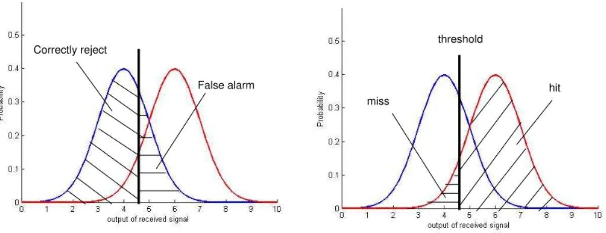
a criterion, different criterion will bring up different decision. There are three basic detection criterion: Bayes Hypothesis Testing, Minimax Hypothesis Testing and Neyman Pearson Hypothesis Testing.[3] In the Bayes criterion, we need the prior probability of

H0and H1 first, and then determine the cost of miss, hit, false alarm, and correctly reject

(see Figure 2.1) respectively. Finally, make decision by minimum cost. In the Minimax criterion, there is no information of prior probability, therefore, the prior probability will be a parameter of the cost function. We make decision by minimize the maximum of conditional expected costs. However, in many problems of practical interest, the imposition of a specific cost structure on the decision isn’t possible or desirable. In such

Correctly reject

False alarm hit

miss

threshold

Figure 2.1: Pulse shaping of signal pass VSB filter.

applications, an alternative design criterion, known as the Neyman Pearson criterion, is often imposed.

2.1

Neyman Pearson Criterion

In testing H0 and H1, there are two types of errors that can be made: H0 can be

falsely rejected or H1 can be falsely rejected. The first error is called a false alarm, and

the second one is called a miss. Obviously, the design of threshold for H0 versus H1

involves a trade-off between the probabilities of these two errors, since one can always be made arbitrarily small at the expense of the other. The Bayes and minimax criteria are two different ways to trading them off. For a decision rule δ, the probability of the

type one error is called false alarm probability (Pf), and the type two error is called

miss probability (Pm). However, it is more often discussed by detection probability.

(Pd = 1 − Pm) The Neyman Pearson criterion for making this trade-off is to place a

bound on the Pf and then to minimize the Pm within this constraint.

max

δ Pd | Pf≦α (2.2)

where α is the above-mentioned bound. The Pd and Pf is given by

Pd=

Z

y∈Γ1(δ)

Pf =

Z

y∈Γ1(δ)

p(y|H0) dy (2.4)

the region Γ1 is decided by decision rule δ to determine the received signal y is

trans-mitted from H1. This decision criterion have been used all over this report.

2.2

Energy detector [4]

Energy detection has been adopted as an alternative spectrum sensing method for cognitive radios due to its low computational complexity and not requiring a priori in-formation of the signal to be detected. Spectrum sensing techniques in cognitive radios can be classified as matched filter detection, energy based detection and cyclostationary based detection. Matched filter detection is a coherent detection method and it max-imizes the signal-to-noise ratio(SNR). However, a priori knowledge of the signal to be detected is necessary in this method. Cyclostationary based detection makes use of the periodicity of the signal’s statistical characteristics, but it is a computationally expensive method. Although energy detectors suffer from noise level ambiguities and require more samples than matched filter detectors, their easy implementation makes it an attractive method in spectrum sensing.

BPF

BW=W=1/T | |2

Н|

|

t=nT,n=1,2,…N r ( t )

r [n]

Figure 2.2: Energy detector.

As illustrated in Figure 2.2, given N = T W received samples, the energy based detection solution for this problem is to find a decision statistic.

T =

N

X

n=1

|r[n]|2 ≷ τ (2.5)

distribution for H1. T σ2 ∼ ½ χ2_{(2N ) H} 0 χ′2_{(2N, N} s2 σ2) H1 (2.6) that the threshold τ is decided as:

τ = σ2 χ2−1_{(1 − P}f, 2N ) (2.7)

where χ2−1 _{is the inverse chi-square cumulation distribution function. It is clearly that}

we need the correctly noise information σ2 _{to decide the threshold, or the expected}

false alarm value Pf couldn’t be achieved. The energy detector would suffer from noise

uncertainty seriously.

2.3

Signal of digital television [6]

CR technologies are attracting and exploding interests in the standardization body of IEEE 802.22. In this body, the coexistence feasibility has been discussing that the communication systems using CR technologies could share with TV stations at TV fre-quency bands. In this section, we mathematically simulation the 8-VSB system model used for the Advanced Television Systems Committee (ATSC) standard.

For over fifty years, National Television Systems Committee (NTSC) has successfully served as the television transmission standard in the United States. Over the years, this system has proven to be very rugged and reliable, providing useful pictures even in severe environments. The main reason for this rugged behavior is the use of supplementary synchronization. However, the cost of this performance is high, both in terms of power and bandwidth efficiency, and does not prevent picture impairment with the introduc-tion of interference.

The advancement of technology now allows the transmission of digital television (DTV) in the same 6MHz bandwidth currently used by NTSC. As described in ATSC A/54 [5], the symbol rate of DTV signal is related to NTSC scanning and color frequen-cies. It simplify receiver design to include both DTV and NTSC decoding capabilities.

The digital transmission offers improved video and audio reception, with none of the usual impairments seen in analog transmission; e.g., multipath, white noise, or impulse noise. The same philosophy used in NTSC can be applied in the design of digital trans-mission systems. It is generally known that digital signals remain error free when the added noise does not increase the signal above the data slice levels. When the noise in-creases to levels that cause errors to occur, the powerful forward error-correction (FEC) schemes, like trellis coding and Reed-Solomon coding, still provide error free operation down to low SNR. The DTV system behavior can be achieved at much better power and bandwidth efficiencies than NTSC.

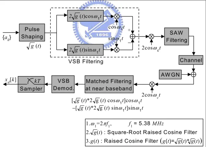
{a_k} Pulse Shaping cosω₁t + sinω₁t SAW Filtering Channel AW GN 2cosω_ct 2 g (t)cosω₁t 2 g (t)sinω₁t g (t) Matched Filtering at near baseband VSB Dem od. kT Sam pler x_d[k] 1.ω₁=2π f₁, f₁= 5.38 MHz

2. g(t) : Square-Root Raised Cosine Filter

[ g (t)*2 g (t) cosω₁t]cosω₁t

[ g (t)*2 g (t) sinω₁t]sinω₁t

3.g(t) : Raised Cosine Filter

(

)

VSB Filtering

2cosω_ct

G

G

2. VSB Filtering and Up-Converting

up-converted with the near-bas

corresponding to half of the sy

procedure for VSB filtering (Fig

3(b)) in the frequency domain.

Figure 2.3 depicts a functional block diagram of the overall passband VSB system for the ATSC DTV standard. We present simulation as the baseband equivalent signal simplified from the passband signal just doing the first two block, the Pulse Shaping and the VSB Filtering of Figure 2.3.

Let {ak} be an information symbol sequence and s(t) a continuous time signal

com-prised of the information symbols, we obtain s(t) =

∞

X

k=0

akδ(t − kT ) (2.8)

where T is the symbol duration of 0.093µs in the ATSC DTV standard in which the symbol rate is 10.76 MHz, in order to avoid inter-symbol interference (ISI), a pulse-shaping filter satisfying the Nyquist criterion is used at the transmitter. We use the square root raised cosine (SRRC) filter √g(t) (see Figure 2.4). The pulse-sahped signal x(t) is given by x(t) = s(t) ∗√g(t) = ∞ X k=0 ak√g(t − kT ) (2.9)

where ∗ denotes a convolution operator. and √g(t) is described below:

√_{g(t) =} β πTs cos[(1 + β)π t Ts] + sin[(1−β)π t Ts] 4β_Tst 1 − (4βTts) 2 (2.10)

where β is a real number in the interval [0, 1] that determine the bandwidth of the

spectrum that the spectrum is zero for |f| > 1+βTs . In the DTV system, The signal

bandwidth of standard is denoted as f1 = _2T1 = 5.38MHz, that β would be given by

(6−5.38)/2

5.38 ≃ 0.0576. The pulse-shaped signal is filtered by the VSB filter. The resulting

baseband complex signal can be obtained as

xvsb(t) = x(t) ∗ 2√g(t)ej2πf1t (2.11)

Figure 2.5 and 2.6 are simulation of the pulse shaping of VSB signal. It is clearly to know the VSB signal would have highly correlation to the neighborhood bits. There is considerable difference from the original pulse shaping of SRRC which almost without correlation.

−10 −9 −8 −7 −6 −5 −4 −3 −2 −1 0 1 2 3 4 5 6 7 8 9 1010 0

1

time (symbol duration T)

amplitude

−10−9 −8 −7 −6 −5 −4 −3 −2 −1 0 1 2 3 4 5 6 7 8 9 10 11 12 13 14 1515 0

1

time (symbol duration T)

amplitude

Figure 2.4: Square root raise cosine pulse shaping.

−10 −9 −8 −7 −6 −5 −4 −3 −2 −1 0 1 2 3 4 5 6 7 8 9 1010 0

0.5

time (symbol duration T)

amplitude −10 −9 −8 −7 −6 −5 −4 −3 −2 −1 0 1 2 3 4 5 6 7 8 9 10 −0.4 0 0.4 amplitude

time (symbol duration T)

Figure 2.5: Pulse shaping of signal pass VSB filter. The left one is real part signal and the right one is the imaginary part signal.

−9 −8 −7 −6 −5 −4 −3 −2 −1 0 1 2 3 4 5 6 7 8 9 1010 0

0.5

amplitude

time (symbol duration T)

−10−9 −8 −7 −6 −5 −4 −3 −2 −1 0 1 2 3 4 5 6 7 8 9 10 11 12 13 14 15 0.5

time (symbol duration T)

amplitude

2.4

SUI channel model

The SUI (Stanford University Interim) channel models will be used in our study of the performance of various algorithms. This model allows many possible combinations of parameters to provide a variety of channel descriptions. A set of 6 typical channels is selected for the three typical terrain types. These models are developed for use in simulations, design, development and testing of technologies suitable for broadband wireless applications. Typically scenario for the SUI models are as follows.

• Cells are less than 10 km in radius for a variety of terrain and tree density types. • Under-the-eave/window or rooftop installed directional antennas (2 − 10 m) at the

receiver

• 15 − 40m BTS antennas

• High cell coverage requirement (80 − 90%)

Table 2.1: SUI-1 channel model definition.

SUI-1 channel Tap 1 Tap 2 Tap 3 Units

Delay 0 0.4 0.9 µs Power(omni ant.) 0 -15 -20 dB 90% K Factor(omni ant.) 4 0 0 dB 75% K Factor(omni ant.) 20 0 0 dB Power(300 _{ant.) 0 -21 -32 dB} 90% K Factor(300 _{ant.) 16 0 0 dB} 75% K Factor(300 _{ant.) 72 0 0 dB} Doppler 0.4 0.3 0.5 Hz

The parameters of the six SUI channels (Figures 2.1 - 2.6), including the propagation scenario that led to this specific set, can be found in the referenced document [7]. The definition of the SUI-3 channel (omni antenna) which is used for our simulations.

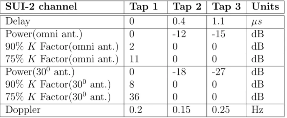
Table 2.2: SUI-2 channel model definition.

SUI-2 channel Tap 1 Tap 2 Tap 3 Units

Delay 0 0.4 1.1 µs Power(omni ant.) 0 -12 -15 dB 90% K Factor(omni ant.) 2 0 0 dB 75% K Factor(omni ant.) 11 0 0 dB Power(300 _{ant.) 0 -18 -27 dB} 90% K Factor(300 _{ant.) 8 0 0 dB} 75% K Factor(300 _{ant.) 36 0 0 dB} Doppler 0.2 0.15 0.25 Hz

Table 2.3: SUI-3 channel model definition.

SUI-3 channel Tap 1 Tap 2 Tap 3 Units

Delay 0 0.5 1 µs Power(omni ant.) 0 -5 -10 dB 90% K Factor(omni ant.) 1 0 0 dB 75% K Factor(omni ant.) 7 0 0 dB Power(300 _{ant.) 0 -11 -22 dB} 90% K Factor(300 _{ant.) 3 0 0 dB} 75% K Factor(300 _{ant.) 19 0 0 dB} Doppler 0.4 0.4 0.4 Hz

Table 2.4: SUI-4 channel model definition.

SUI-4 channel Tap 1 Tap 2 Tap 3 Units

Delay 0 1.5 4 µs Power(omni ant.) 0 -4 -8 dB 90% K Factor(omni ant.) 0 0 0 dB 75% K Factor(omni ant.) 1 0 0 dB Power(300 _{ant.) 0 -10 -20 dB} 90% K Factor(300 _{ant.) 1 0 0 dB} 75% K Factor(300 _{ant.) 5 0 0 dB} Doppler 0.2 0.15 0.25 Hz

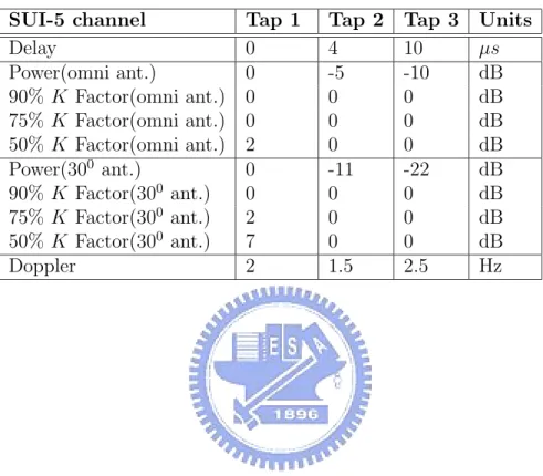
Table 2.5: SUI-5 channel model definition.

SUI-5 channel Tap 1 Tap 2 Tap 3 Units

Delay 0 4 10 µs Power(omni ant.) 0 -5 -10 dB 90% K Factor(omni ant.) 0 0 0 dB 75% K Factor(omni ant.) 0 0 0 dB 50% K Factor(omni ant.) 2 0 0 dB Power(300 _{ant.) 0 -11 -22 dB} 90% K Factor(300 _{ant.) 0 0 0 dB} 75% K Factor(300 _{ant.) 2 0 0 dB} 50% K Factor(300 _{ant.) 7 0 0 dB} Doppler 2 1.5 2.5 Hz

Table 2.6: SUI-6 channel model definition.

SUI-6 channel Tap 1 Tap 2 Tap 3 Units

Delay 0 14 20 µs Power(omni ant.) 0 -10 -14 dB 90% K Factor(omni ant.) 0 0 0 dB 75% K Factor(omni ant.) 0 0 0 dB 50% K Factor(omni ant.) 1 0 0 dB Power(300 _{ant.) 0 -16 -26 dB} 90% K Factor(300 _{ant.) 0 0 0 dB} 75% K Factor(300 _{ant.) 2 0 0 dB} 50% K Factor(300 _{ant.) 5 0 0 dB} Doppler 0.4 0.3 0.5 Hz

Chapter 3

Multi-tone Detector

In this chapter, we investigate the joint forward and backward consecutive mean excision algorithm for spectrum sensing. The methods are based on a set of energy measurement samples, that is, the outputs of the energy detectors. This method does’t require the knowledge of the noise level to decide the threshold of detection. Further-more, it doesn’t require fixed vacant channels nor signal-free guard bands. The proposed approach does require a few vacant channels but they do not have to be at fixed fre-quency bands. Since it detect multiple frefre-quency bands at at one time, we call it a multi-tone detector.

3.1

System model of multi-tone detector

The sensing device is assumed to perform energy measurements of the candidate frequencies (see Figure 3.1). Denote the energy detector outputs

zi =

Z

r2_{(t) dt |} t=iT , i=1,2,3... (3.1)

where {r(t)} is the received time domain signal. We have to compare each energy detector output with a threshold τ to decide whether signal exists, i.e., the frequency band is occupied. The traditional energy detector would detect as

where tau would be decided with the information of noise variance, it has already ex-plained in details in chapter 2. However, the difference of now from the traditional energy detector is that we have a set of energy detector outputs, assuming that each output channel survive from similar noise environment. We could use these multiple materials to find a new algorithm to detect without information of noise variance.

BPF BW=1/T, fc1 | | 2 t=NT

∫

dt

∫

dt

∫

dt

∫

_dt

∫

dt

Figure 3.1: Energy detector array for multi-tone detector.

3.2

The FCME algorithm

First, we reorder zi in an ascending order with yi, turn our criterion to the ratio of

adjoining yi (see Figure 3.2). that is

T = yi+1

yi ≷ τ (3.3)

If T ≧ τ , the detector decides that the channel of output yi+1 have signal existed, so

as to avoid noise level ambiguities. The threshold τ′ _{is set using the Neyman-Pearson}

Criterion, too. Therefore, it is set assuming the noise-only case and determining the probability that samples exceeds the threshold.

Channel

Energy detector output

1 2 3 4 5 6 7 8 9 10 11 12 13 14 15 16 17 18 19 20

Channel

Sorted Energy detector output

5 2 12 13 11 6 10 16 1 7 3 4 18 20 19 14 9 8 15 17

sorting

Figure 3.2: Energy detector output for multi-tone detector. The output of channels with signal would be accumulated with larger power than which of signal free channels. It can justify easily that channels with larger outputs would have signal existed.

The spectrum sensing problem can be viewed as a binary detection problem which statistic in each hypotheses can be summarized as

T = yi+1

yi ∼

½

F (2N, 2N, 0) H0

F (2N, 2N, λ) H1 (3.4)

where F (ν1, ν2, λ) is a F-distribution with noncentral parameter λ, that is the SNR of

received signal, and degree of freedom ν1, ν2, that is sample numbers of received signal.

Using this ratio statistic, the parameter of noise level would be eliminate,so that we can avoid the uncertainty of noise level to harm our detection performance. A random variate of F-distribution arises as the ratio of two chi-squared variates:

U1/ν1

U2/ν2

(3.5) where

• U1 is chi-square distributions with ν1 degrees of freedom, noncentral parameter λ.

• U2 have chi-square distributions with ν2 degrees of freedom.

The probability density function for the noncentral F-distribution is p (T |H0) = ∞ X 0 eλ/2_(λ/2)k B(ν2 2 , ν1 2 + k)k! (ν1 ν2 )ν12 +k( ν2 ν2+ ν1f )ν1+ν22 +k (T ) ν1 2 −1+k (3.6) where B(x, y) = Γ(x)Γ(y) Γ(x + y) (3.7)

that Γ(.) is the gamma function.

Use the Neyman-Pearson Criterion to set threshold τ′_:

Pf =

Z ∞

τ′

p (T |H0) dT (3.8)

where Pf is the false alarm probability system want to achieve. Moreover, the detection

performance could quantify by deflection coefficient(distance between two hypothesis). If

the deflection coefficient is larger, there is larger detection probability at the assigned Pf.

With different variance of hypothesis H0 and H1, there is modified deflection coefficient

defined as equation 3.9. We can find that the more distance from the mean of two hypothesis and the smaller variance both of them would bring the larger deflection coefficient d, that is, better detection performance.

d ≡ E[H1]

pV AR[H1]

− E[H0]

pV AR[H0]

(3.9)

However, we know the mean and variance of F-distribution would be ν2(ν1+λ)

ν1(ν2−2) and

2(ν1+λ)2+(ν1+2λ)(ν2−2)

(ν2−2)2(ν2−4) (

ν2

ν1)

2_{, so that the performance of this detector would be limited to}

the SNR and number of samples N . For the ratio statistic T = yi+1_y

i =

U1/ν1

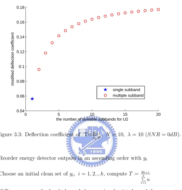
U2/ν2, fortunately,

if we increase the degrees of freedom of U2, the deflection coefficient would increase, too.

(see Figure 3.3) Therefore, the ratio statistic is changed to T = _j<iyi

P

j=1

yj

(3.10)

And then, we can join the recursive algorithm in our sensing device. The sensing algo-rithm is emphasized below:

0 5 10 15 20 0.04 0.06 0.08 0.1 0.12 0.14 0.16 0.18

the number of aviliable subbands for U2

modified deflection coefficient

single subband multiple subband

Figure 3.3: Deflection coefficient of T=yi+1

P yi, N = 10, λ = 10 (SN R = 0dB).

1. Reorder energy detector outputs in an ascending order with yi

2. Choose an initial clean set of yi, i = 1, 2.., k, compute T = ykk+1

P

i=1

yi

3. If T < τ , we say the k + 1 channels has no signal existed , and than repeat step 2

as adding the yk+1 to the clean set.

If T > τ , stop recursive algorithm and we say the k+1 to the last channel all have signal existed.

where

τ = F−1_{(1 − P}f, 2N, 2N k, λ) (3.11)

F−1 _{is inverse F cumulation distribution function. The threshold is decided without}

the effect of the noise variance clearly. This algorithm called forward consecutive mean excision algorithm (FCME) has been used in outlier detection, impulse detection, and

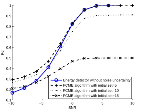
interference suppression before. Note that, it is able to perform further processing on the frequency bands energy detection finds occupied, e.g., separating licensed users form unlicensed ones. However, the FCME algorithm must have enough vacant channels, i.e., the assumed initial clean set is actually signal free. In the case that there is channels with signal in the initial set, they can’t be detected anymore. From Figure 3.4, it shows too large initial set would bring a bound of the detection probability. On the other hand, the smaller initial clean set could avoid most of these undetectable case, but it means more iterations are needed.

−10 −5 0 5 10 0.1 0.2 0.3 0.4 0.5 0.6 0.7 0.8 0.9 1 SNR Pd

Energy detector without noise uncertainty FCME algorithm with initial set=5 FCME algorithm with initial set=10 FCME algorithm with initial set=15

Figure 3.4: Detection probability of FCME algorithm with different initial clean set. Simulation with QPSK signal passing by SUI3 fading channel in 20 different frequency bands. The prior probability of signal existing or not is 50%.

3.3

The FBCME algorithm

To reduce this effect of too large initial clean set, we join the backward consecutive mean excision algorithm (BCME). Both CME algorithm operate iteratively by calculat-ing new thresholds of new clean set until stable. The FCME algorithm is addcalculat-ing new members to the clean set and the BCME algorithm would take out members from the clean set. We use this feature of BCME algorithm to overcome the problem of choos-ing too large initial clean set. However, the BCME algorithm couldn’t work well itself. Note the threshold of CME algorithm is computed by the noise only clean set. If there

are yk+1 with signal existing in this set, the threshold isn’t correct enough. Although

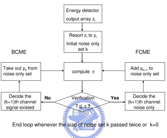
we can use the BCME algorithm to reject the obvious elements with signal, too large initial clean set still make too great threshold which cause the smaller detection proba-bility and false alarm probaproba-bility. We propose a new algorithm by combining the FCME and BCME to improve the defect of original algorithm. The total sensing algorithm is rewrote below and is called joint forward and backward consecutive mean excision algorithm (FBCME):

1. Reorder energy detector outputs in an ascending order with yi

2. Choose an initial set of yi, i = 1, 2.., k, compute T = ykk+1

P

i=1

yi

3. If T < τ , we say the k + 1 channels has no signal existed , and than repeat step 2

as adding the yk+1 to clean set, that is FCME algorithm.

If T > τ , we say the k+1 to the last channel all have signal existed and repeat

step 2 with taking out yk from the clean set, that is BCME algorithm.

Recursively do this algorithm until all the channels are detected. To avoid infinite cycle, the algorithm records the size of k. If this k have computed before, stop recursive algorithm and output decision.

Energy detector output array z_i

Resort z_ito y_i Initial noise only

set k compute ӻ Verification TЉӻ? Yes No Decide the (k+1)th channel noise only Add y_k+1 to noise only set

Decide the (k+1)th channel

signal existed Take out y_kfrom noise only set

End loop whenever the size of noise set k passed twice or k=0

FCME

BCME

Figure 3.5: Flow chart of proposed FBCME algorithm.

The proposed FBCME algorithm could reduce the undetectable situations by the original FCME algorithm, but it still has a least one vacant channel amongst the set of sensed channels. The performance of FBCME algorithm is similar to the FCME algorithm with initial noise set k=1, however, the FBCME algorithm costs less iterations. From Figure 3.6, 3.7 and 3.8, we can see the detection probability of FCME and BCME algorithm does not effected by noise uncertainty in certainty. However, the false alarm probability of FCME and FBCME algorithm is unable to reach its expected value. The FCME algorithm has the higher false alarm probability at low SNR and the lower false alarm probability at high SNR, and the FBCME algorithm would cause higher false

−10 −5 0 5 10 0.1 0.2 0.3 0.4 0.5 0.6 0.7 0.8 0.9 1 SNR Pd

Optimal energy detector fcme algorithm fbcme algorithm

Figure 3.6: Detection Probability of FBCME algorithm. Simulation with DTV signal passed by SUI3 fading channel in 20 different frequency bands. The prior probability of signal existing or not is 50%. The optimal energy detector means that energy detector without noise uncertainty.

obviously caused by the initial clean set with signal terms. There are still two reasons might cause error. One is that at low SNR the miss detection would make the clean set include signal term, so that the threshold would higher than original ones. However,

from simulation results, we find the Pf is larger than our expected value with both

FCME and FBCME algorithm at low SNR . Therefore, the first reason doesn’t affect our performance seriously. The other reason might happen is because that when we

reorder the energy detector output zi in an ascending order yi, they are not iid samples

anymore. When we replace the order statistic distribution should happen in fact with the chi-square distribution, it causes error in computing the threshold. Although these CME algorithms could detect without noise information, it has little fault in probability

of false alarm. Fortunately, note the error of Pf in CME algorithm is smaller than which

−150 −10 −5 0 5 0.1 0.2 0.3 0.4 0.5 0.6 0.7 0.8 0.9 1 SNR Pd

Optimal energy detector

FCME algorithm−2dB noise uncertainty Energy detector−2dB noise uncertainty FBCME algorithm−2dB noise uncertainty

Figure 3.7: Detection probability of FBCME algorithm suffered by noise uncertainty. Simulation with DTV signal passed by SUI3 fading channel in 20 different frequency bands. The prior probability of signal existing or not is 50%.

−15 −10 −5 0 5 0.05 0.1 0.15 0.2 0.25 0.3 0.35 0.4 SNR Pf

Optimal energy detector

FCME algorithm−2dB noise uncertainty Energy detector−2dB noise uncertainty FBCME algorithm2dB noise uncertainty

Figure 3.8: False alarm probability of FBCME algorithm suffered by noise uncertainty. Simulation with DTV signal passed by SUI3 fading channel in 20 different frequency bands. The prior probability of signal existing or not is 50%.

Chapter 4

Single-tone Detector

The multi-tone detector referred last chapter need multiple receiver blocks to detect distinct channels simultaneously. In later chapters, we discuss that If there is only one channel to be sensed at a time, what algorithm could work well in the major premise which the secondary user doesn’t known any information of the primary user, this is to say, we want to propose a method to signal detection which could be used for various sensing applications without knowledge of the signal, the channel and the noise level.

4.1

Eigenvalue based sensing algorithms

This sensing algorithm is present for the IEEE 802.22 WRANs [12]. Since the max-imum and minmax-imum eigenvalue of the sample covariance matrix of the received signal contain the signal and noise information, respectively. Based on random matrix theories, the information is quantized and then used for signal detection. The threshold is found by using the constant false alarm without information of noise level.

Let r[n], n = 0, 1, 2... be the received signal samples, and define

x =         r(n) r(n + 1) r(n + 2) . . . r(n + L) r(n + 1) r(n + 2) . . . ... r(n + 2) r(n + 3) . . . ... ... . .. . .. ... r(n + M ) r(n + M + 1) _{· · · · · · · · ·}        

Compute R = xxH_{, and then obtain the maximum and minimum eigenvalues of the}

matrix R, λmax and λmin. If λ_λmax_min > γ, signal exists, otherwise, signal not exists.

The threshold γ is computed as:

γ = (1 +pM/L) 2 (1 −pM/L)2[1 + (√L +√M )−2/3 (M L)1/6 F −1 1 (1 − Pf)] (4.1)

where F1 is the Tracy-Wisdom distribution of order 1. The Tracy-Wisdom distribution

were found by Tracy and Wisdom as a limiting law of the largest eigenvalue of certain random matrices. The value of the Tracy-Wisdom distribution is given in Table 4.1.

Table 4.1: Numerical table for the Tracy-Wisdom distribution of order 1.

t -3.9 -3.18 -2.78 -1.91 -1.27 -0.59 0.45 0.98 2.02

F1(t) 0.01 0.05 0.10 0.30 0.50 0.70 0.90 0.95 0.99

For complex signal, the difference is that the function F1 should be replaced by F2,

the CDF of the Tracy-Wisdom distribution of order 2. We use the performance of this algorithm referred as IEEE 802.22 meeting document to compare with our proposed algorithm in later section.

4.2

Ratio detector

The goal wanted to achieve is to decide whether the signal exists or not without information of noise variance. At the beginning, the basic concept of this algorithm is to produce two outputs with noise information, and then deduct them, receive the result not including the noise information. For example, if we could get an output A with

value 3σ2 _{and another output B with value 20σ}2_{, although each of them has information}

of noise level, their quotient does not. The first output A we’ve already have is the energy detector output, and then we should produce an output different from energy detector but still have information of noise variance. At chapter 2, we’ve show that the DTV signals have very strong correlation from the nearby bits. Consult the method

which utilizes the autocorrelation among signals have been used to detect signal with low power . [14] (see Figure 4.1)

Delay KT t=NT Power sampler processor

∫

dt

Figure 4.1: Mathematical model of a real time autocorrelation detector.[3]

Consider the output after the correlator y [K]. It is suitable the central limit theory for large N , we can derive the y [K] with gaussian distribution in the situation of noise only and with signal, respectively.

y [K] = t=N T Z t=KT r(t)r(t − KT ) dt|t=N T ≃ N −1 X n=K r[n]r[n − K] (4.2)

The noise only case H0:

E{ y [K] } = E{ N −1 X n=K r[n]r[n − K] } = N −1 X n=K E{ w[n]w[n − K] } = 0 (4.3) V ar{ y [K] } = E{ N −1 X n=K (r[n]r[n − K]) N −1 X m=K (r[m]r[m − K])∗ } − E{ y [K] }2 = N −1 X n=K E{ w[n]w[n]∗w[n − K]w[n − K]∗ } + N −1 X n=K N −1 X m6=n E{ w[n]w[m]∗w[n − K]w[m − K]∗ } = (N − K)(σ 4 2 + σ4 2 i) (4.4)

The alternative case H1: E{ y [K] } = E{ N −1 X n=K r[n]r[n − K] } = N −1 X n=K E{ (s[n] + w[n])(s[n − k] + w[n − K]) } = 0 (4.5) V ar{ y [K] } = E{ N −1 X n=K (r[n]r[n − K]) N −1 X m=K (r[m]r[m − K])∗ } − E{ y [K] }2 = N −1 X n=K E{(s[n] + w[n])(s[n] + w[n])∗(s[n − K] + w[n − K]) (s[n − K] + w[n − K])∗ } + N −1 X n=K N −1 X m6=n E{(s[n] + w[n])(s[m] + w[m])∗ (s[n − K] + w[n − K])(s[m − k] + w[m − k])∗ } = (N − K)(s 4 2 + σ4 2 + s 2_σ2_{)(1 + i)} (4.6) where s[n] and w[n] denotes signal samples and noise samples. They are assumed to be

iid zero mean signal and white gaussian noise in order to derive simplistically. s2 _{is the}

signal power, and σ2 _{is the noise power. By central limit theory, we can get:}

H0 : √y [K] N − K ∼ N(0, σ4 2 ) + N (0, σ4 2 )i H1 : √y [K] N − K ∼ N(0, s4 2 + σ4 2 + s 2_σ2_{) + N (0,}s4 2 + σ4 2 + s 2_σ2_)i (4.7) After a power sampler processer, there is

H0 : 2 σ4 K=M X K=1 ¯ ¯ ¯ ¯ y [K] √ N − K ¯ ¯ ¯ ¯ 2 ∼ χ2(2M ) H1 : 2 s4_{+ σ}4_{+ s}2_σ2 K=M X K=1 ¯ ¯ ¯ ¯ y [K] √ N − K ¯ ¯ ¯ ¯ 2 ∼ χ2(2M ) (4.8)

BPF BW=1/T | |2 Power sampler processor t=pm₁T

∫

dt

Figure 4.2: Mathematical model of energy detector output through a power sampler processer.

Another output is the energy detector output through a power sampler processer. (see Figure 4.2) The distribution is expressed below. Nevertheless, there is still central limit theory used to approximate the energy detector output before the power sampler processer x[p] from chi-square distribution to gaussian distribution.

H0 : 1 σ2x[p] ∼ χ 2_(2m 1) ∼ N(2m1, 4m1) H1 : 1 σ2x[p] ∼ χ ′2_(2m 1, m1s2 σ2 ) ∼ N(2m1+ m1s2 σ2 , 4m1+ 4m1s2 σ2 ) (4.9) H0 : 1 m2σ4 m2 X p =1 µ x[p] √_m 1 ¶2 ∼ χ′2(m2, m1σ4 σ4 ) H1 : 1 m2(σ4+ 2s2σ2) m2 X p =1 µ x[p] √_m 1 ¶2 ∼ χ′2(m2, m1(s2 + σ2)2 σ4 ) (4.10)

Hence, the ratio of energy detector output and correlator output would be noncentral chi-square distribution as the equation 4.11. What merits attention is that there is no noise variance in the noise only case, so that it doesn’t need any noise information to decide the threshold. The mathematical model is shown at Figure 4.3.

BPF BW=1/T | |2 Power sampler processor t=pm₁T

∫

dt

∫

dt

Figure 4.3: Mathematical model of ratio detector.

H0 : M m2 m2 P(√x[n]_m 1) 2 M P |√y[K] N −K| 2 ∼ F (m2, 2M, m1) H1 : M m2 (1 + s 4 σ4 _{+ 2s}2_σ2) m2 P(√x[n]_m 1) 2 M P |√y[K] N −K| 2 ∼ F (m2, 2M, m1(1 + s4 σ4_{+ 2s}2_σ2)) (4.11) The ratio detection problem would be wrote as:

T = m2 P(√x[n]_m 1) 2 M P |√y[K] N −K| 2 ≷ γ

If T > γ, signal exists, otherwise, signal not exists. Where the threshold γ is decided as:

γ = m2

M F

−1_{(1 − P}

f, m2, 2M, m1)

Unfortunately, although we can decide the threshold without noise power by Neyman Pearson criterion, we could find this detector has very poor detection performance.(see Figure 4.4, 4.5) This detector would have similar mean for the noise only case and the alternative case, especially at low SNR. In addition, the variance of both cases rises with their noncentral parameter, it goes up whenever noise power or signal power increase.

−300 −25 −20 −15 −10 −5 0 0.1 0.2 0.3 0.4 0.5 0.6 0.7 0.8 0.9 1 SNR Pd Ratio detector

energy detector without noise uncertainty

Figure 4.4: Detection probability of ratio detector. Simulation with QPSK signal passing through SUI3 fading channel.

−300 −25 −20 −15 −10 −5 0 0.1 0.2 0.3 0.4 0.5 0.6 0.7 0.8 0.9 1 SNR Pf Ratio detector

Energy detector without noise uncertainty

Figure 4.5: False alarm probability of ratio detector. Simulation with QPSK signal passing through SUI3 fading channel.

0 1 2 3 4 5 0 0.02 0.04 0.06 0.08 0.1 0.12 0.14 0.16 0.18 0.2

probability density function

F(100,100,0) F(100,100,50) F(100,100,100) F(100,100,200) 0 1 2 3 4 5 0 0.02 0.04 0.06 0.08 0.1 0.12 0.14 0.16 0.18 0.2

Probability density function

F(100,100,0) F(10,10,0) F(10,100,0) F(100,10,0)

Figure 4.6: Probability density function of noncentral F distribution. The left figure is noncentral F distribution with the same degrees of freedom and different noncentral parameter. The right one is F distribution with different degrees of freedom.

4.3

Modified Ratio Detector

From Figure 4.6, it’s clear to know the larger noncentral parameter of noncentral F distribution would make the distribution spread, that is, the variance would grow. Be-sides that, it tells us that choosing the match degrees of freedom would bring the more sharp distribution. If we could design a detector with more sharp distribution in each hypothesis, it will be more clearly distinguish between these two hypothesis. Therefore, the performance will be better than original radio detector.

Add the random sequence P [n] with element {1,-1} which each element has equal probability to our ratio detector model and choose the match degrees of freedom, i.e.

make m2 = 2M . The intension of P [n] is to force the noncentral parameter of detector

to be zero. This is a modified ratio detector. (see Figure 4.7) The threshold would be decided by constant false alarm probability criterion and without the information of noise variance yet. We will show the performance by simulation to prove the detection probability of this modified ratio detector is similar to which of the maximum and minimum eigenvalue based algorithm (SVD detecotr) proposed in the 802.22 meeting document.

BPF BW=1/T | | 2 Delay KT Power sampler processor t=kT

∫

dt

∑

∫

dt

Figure 4.7: Mathematical model of ratio detector.where P [n] is a random sequence with element {1,-1}, each element has equal probability.

H0 : 2m2 M M P |√y[k] N −K| 2 m2 P(√z[n]_m 1) 2 ∼ F (2M, m2, 0) (4.12) H1 : [2 − s 4 (s2_{+ σ}2₎2] m2 M M P |√y[k] N −K| 2 m2 P(√z[n]_m 1) 2 ∼ F (2M, m2, 0) (4.13) The modified ratio detection problem would be wrote as:

T = M P |√y[k] N −K| 2 m2 P(√z[n]_m 1) 2 ≷ γ

If T > γ, signal exists, otherwise, signal not exists. Where the threshold γ is decided as:

γ = M

2m2

−300 −25 −20 −15 −10 −5 0 0.1 0.2 0.3 0.4 0.5 0.6 0.7 0.8 0.9 1 SNR Pd

Modified ratio detector Optimal energy detector SVD detector

0.5dB noise uncertainty 1dB noise uncertainty 0.1dB noise uncertainty

Figure 4.8: Detection probability of modified ratio detector. Simulation by QPSK signal passing through SUI3 fading channel.

−30 −25 −20 −15 −10 −5 0 0.05 0.1 0.15 0.2 0.25 0.3 0.35 0.4 0.45 0.5 SNR Pf

Modified ratio detector Optimal energy detector SVD detector

Energy detctor with 0.5dB noise uncertainty (12%) Energy detctor with 1 dB noise uncertainty (25%) Energy detctor with 0.1dB noise uncertainty (2%)

Figure 4.9: False alarm probability of modified ratio detector. Simulation by QPSK signal passing through SUI3 fading channel.

−300 −25 −20 −15 −10 −5 0 0.1 0.2 0.3 0.4 0.5 0.6 0.7 0.8 0.9 1 SNR Pd

Modified ratio detector Optimal energy detector SVD detector

0.5dB noise uncertainty (12%) 1dB noise uncertainty (25%) 0.1dB noise uncertainty (2%)

Figure 4.10: Detection probability of modified ratio detector. Simulation by DTV signal passing through SUI3 fading channel. The highly correlation of signal would rise the detection performance significantly.

−30 −25 −20 −15 −10 −5 0 0.05 0.1 0.15 0.2 0.25 0.3 0.35 0.4 0.45 0.5 SNR Pf

Modified ratio detector Optimal energy detector SVD detector

Energy detctor with 0.5dB noise uncertainty (12%) Energy detctor with 1 dB noise uncertainty (25%) Energy detctor with 0.1dB noise uncertainty (2%)

Figure 4.11: False alarm probability of modified ratio detector. Simulation by DTV signal passing through SUI3 fading channel.

In reality, a ratio detector doesn’t have good detection performance. Because that any ratio distribution like student T, F and cauchy distribution are heavy-tailed, it couldn’t separate noise only and signal case clearly as energy detector. We can find by simulation in QPSK signal (see Figure 4.8 and 4.9) that this detector have about 7dB performance loss from optimal energy detector which doesn’t suffer from noise uncer-tainty, and in simulation of DTV signal, the highly correlation signal, (see Figure 4.10 and 4.11) there is still about 3dB performance loss. However, the value of ratio detector is to decide threshold without knowledge of noise power. From those simulation results, although the detection probability has injury not very hard in low noise uncertainty (about 2% estimation error), we’ll find the false alarm probability of energy detector is affected seriously. The proposed ratio detector would have much better performance in such environment which hard to get the correct noise information than traditional energy detector.

Chapter 5

Joint estimation and detection

There is an algorithm different form the ratio test in former chapters. Since the energy detector without noise uncertainty would have better performance than ratio test, we propose a new kind of detector that will estimate noise variance before detection, and then use the estimation results to detect.

5.1

Moment estimation

There is no information of signal, channel and noise power as before. We try to estimation the noise power before detection by the statistic of received signals.

BPF BW=1/T | |2

Σ

∫

dt

The statistic of received signal is H1 : 1 σ2x[n] ∼ χ( m1× s2 σ2 , 2m1) H0 : 1 σ2x[n] ∼ χ(0, 2m1) (5.1) By central limit theorem, the statistic can be approximated as

H1 : x[n] ∼ N(m1(s2+ σ2), m1(σ4+ 2s2σ2))

H0 : x[n] ∼ N(m1σ2, m1σ4)

(5.2)

that the signal power s2 _{and noise power σ}2 _{can be solved by the mean and variance of}

x[n], where E = E{x[n]}_m1 , var = V AR{x[n]}_m1 .

½ s2_{+ σ}2 _{= E}

σ4_{+ 2s}2_σ2 _{= var} (5.3)

So that, the signal power s2 _{and noise power σ}2 _{would be}

s2 = √E2_{− var (5.4)}

σ2 _{= E −}√E2_{− var (5.5)}

Actuality, there is no exactly value of mean and variance. We have to estimate E and V AR first. There is a minimum variance unbias estimation which achieve the Cramer-Rao Lower Bound [15] with the probability density funtion (PDF) of energy detector

output described as fx(x) = {_2πm1_1var exp[−(x−m1E)

2

2m1var ]}

m2_{. The estimation of E and var}

would be ˆ E = 1 m1× m2 m2 X x[n] (5.6) ˆ var = 1 m1× (m2− 1) m2 X (x[n] − m1E)ˆ 2 (5.7)

Since all our information is embodied in the observed data and the underlying PDF for that data, it is not surprising that the estimation accuracy depends directly on

its PDF. Intuitively, the ”sharpness” of the PDF determines how accurately we can estimate the unknown parameter. To quantify this notion observe that the sharpness is effectively measured by the negative of the second derivative of the logarithm of the likelihood function at its peak. It is called Cramer-Rao Lower Bound (CRLB). If the variance of estimation achieve the CRLB, it will be the minimum variance estimation.

The variance of ˆE and ˆvar are described as follow

V AR[ ˆE] = 1 m1 × m2 var (5.8) V AR[ ˆvar] = 1 m2 var2 (5.9)

It is obviously, the estimation result converge as m1 and m2 increase. i.e. the estimation

would be more correct when there are more energy detector output samples.(see Figure

5.2) However, the convergence of ˆvar isn’t faster enough, the estimation of noise power

σ2 _{would have estimation error especially in H}

0 case. With the estimation error, the

detection performance is bad as energy detector with noise uncertainty.

103 104 105 106 −0.4 −0.3 −0.2 −0.1 0 0.1 0.2 0.3 0.4

error ratio of estimated noise

TW

−0.080 −0.06 −0.04 −0.02 0 0.02 0.04 0.06 0.08 50 100 150 200 250 300 350 400

error ratio of estimated noise m2=10000 E: CRLB 0.00084 SIMU 0.0008159 VAR:CRLB 1.4112 SIMU 1.4685

Figure 5.3: Histogram for error ratio of estimated noise variance σ2 _{in H1 case, AWGN.}

The estimation error would cause about 5% noise uncertainty.

−0.250 −0.2 −0.15 −0.1 −0.05 0 0.05 0.1 500

1000 1500

error ratio of estimated noise for H0 case TW=100000

E: CRLB=0.00004 SIMU=0.0000408 VAR: CRLB=0.0032 SIMU=0.0041

Figure 5.4: Histogram for error ratio of estimated noise variance σ2 _{in H0 case, AWGN.}

The left tail of histogram is caused by equation 5.4 that ˆσ2 _{= ˆE −}p ˆ_E2_{− ˆvar, when E}

converge to σ2 _{faster than s}2 ₌p ˆ_E2_{− ˆvar converge to 0, the estimated noise power σ}2

−30 −20 −10 0 10 20 0.1 0.2 0.3 0.4 0.5 0.6 0.7 0.8 0.9 1 SNR Pd

Optimal energy detector 1dB noise uncertainty Moment estimation

Figure 5.5: Detection probability of energy detector using moment estimation in AWGN.

N=100000, m1=10, m2=10000, the estimation error is about 1dB noise uncertainty.

−30 −20 −10 0 10 20 0.05 0.1 0.15 0.2 0.25 0.3 0.35 0.4 0.45 0.5 0.55 SNR Pf

Optimal energy detector 1dB noise uncertainty Moment estimation

Figure 5.6: False alarm probability of energy detector using moment estimation in

5.2

Momnet estimation in Likelyhood ratio test

The section 5.1 tell us using the results of moment estimation to a energy detector and to simulation its performance. At this section, we use the estimation results to a likelyhood ratio test instead the energy detector and then compare its performance, too. The likelyhood ratio test would make decision by the probability of received signal, i.e,

p(R|H1)p(H1) and p(R|H0)p(H0). where R is the magnitude of received signal sequences.

p(R|H1)p(H1) p(R|H0)p(H0) ≷ 1 (5.10) where p(R|H1) = T W Y i=1 ( Ri σ2 1 e− R2_i+A2 2σ2_{1 I} 0( RiA σ2 1 ) ) (5.11) p(R|H0) = T W Y i=1 ( Ri σ2 0 e− R2_i 2σ2₀ ) (5.12) However, as shown with equation 5.11 and 5.12, the probability of received signal are

described with unknown parameter σ2 _{and A, where A is the magnitude of transmitted}

signal. We will use the results of moment estimation to the likelyhood ratio test.

ˆ A = √4 E2_{− var (5.13)} ˆ σ2 1 = E − √ E2_{− var (5.14)} ˆ σ2 0 = E (5.15)

where E and var denote the sample mean and sample variance.

E = 1 T W T W X x[n] (5.16) var = 1 T W − 1 T W X (x[n] − E)2 (5.17)

Unfortunately, the estimation error isn’t small enough. We will show the simulation results for Figure 5.7 ∼ 5.12.

0 0.2 0.4 0.6 0.8 1 1.2 1.4 1.6 1.8 2 0 50 100 150 200 250 300 350 400 450 500 A The real value of A = 1.4142

Figure 5.7: Histogram for ˆA for H1 case.

0 0.5 1 1.5 2 2.5 0 50 100 150 200 250 300 350 400

Estimated noise variance at H1 case The real value = 1

Figure 5.8: Histogram for ˆσ2

1 for H1 case. 1.4 1.6 1.8 2 2.2 2.4 2.6 2.8 0 50 100 150 200 250 300 350 400

Estimated noise variance for H1 case The real value = 1

Figure 5.9: Histogram for ˆσ2

0 0.2 0.4 0.6 0.8 1 1.2 1.4 0 500 1000 1500 2000 2500 3000 3500 4000 4500

The real value A = 0

Figure 5.10: Histogram for ˆA for H0 case.

0.2 0.4 0.6 0.8 1 1.2 1.4 1.6 0 50 100 150 200 250

Estimated noise variance for H0 case The real value = 1

Figure 5.11: Histogram for ˆσ2

1 for H0 case. 0.7 0.8 0.9 1 1.1 1.2 1.3 1.4 1.5 0 50 100 150 200 250 300 350

Estimated noise variance at H0 case The real value = 1

Figure 5.12: Histogram for ˆσ2

−10 −5 0 5 10 0.1 0.2 0.3 0.4 0.5 0.6 0.7 0.8 0.9 1 SNR Pd

Likelyhood ratio test Optimal energy detector

Figure 5.13: Detection probability of Likelyhood ratio test and energy detector with-out noise uncertainty, simulation with QPSK signal passing through AWGN channel, TW=100. −100 −5 0 5 10 0.1 0.2 0.3 0.4 0.5 0.6 0.7 0.8 0.9 1 SNR Pf

Likelyhood ratio test Optimal energy detector

Figure 5.14: False alarm probability of Likelyhood ratio test and energy detector with-out noise uncertainty, simulation with QPSK signal passing through AWGN channel, TW=100.

Chapter 6

Conclusion

We present blind non-coherent spectrum sensing algorithms in the environments where there is no information of signals, channels, and noise power in various applications for cognitive radio. Our solution to multi-tone detection is called FBCME algorithm. This approach requires a few vacant channels but they do not have to be at fixed frequency bands. There are some error in the false alarm probability from the expected value in our algorithm. However, it is smaller than the effect in an energy detector with noise uncertainty. The other proposed algorithm for single-tone detection is called ratio detector. Although the detection probability of this algorithm is much lower than the energy detector without noise uncertainty, it would be better than energy detector even with little noise uncertainty. A high correlation signal of primary user could improve the detection performance effectively. The ratio detector prevent the detection performance from noise uncertainty, too. In the last chapter, we try to estimation noise variance before detection. Unfortunately, this estimation isn’t accurate enough, the little noise uncertainty would bring large performance loss especially in low SNR.

Bibliography

[1] Joseph Mitola III and Gerald Q. Maguire, Jr, ”Cognitive Radio: Making software more personal”, Aug. 1999

[2] J.Mitola, ”Cognitive radio for flexible mobile multimedia communicaion”, IEEE International Workshop on Mobile Multimedia Communications, pp 3-10, Nov. 1999 [3] H.Vincen Poor, ”An Introduction to Signal Detection and Estimation”

[4] Harry Urkowitz, ”Energy detection of unknown determistic signals”, Proceedings of the IEEE, vol 55, No.4, April 1967

[5] ”ATSC Recommended Practice A/54A: Guide to the Use of the ATSC Digital Television Standard”, Dec. 2003

[6] Hyoung-Nam Kim, Yong-Tae Lee, and Seung Won Kim, ”Mathematical model-ing of VSB-based digital television system”, ETRI Journal, Vol.25, No.1, pp.9-18, Feb.2003

[7] ”Channel model for fixed wireless applications”, IEEE 802.16.3c-01/29r4, July 2001.

[8] Steve Shellhammer, Victor Tawil, Gerald Chouinard, Max Muterspaugh, Monisha Ghosh ”Spectrum Sensing Simulation Model”, IEEE 802.22-06/0028r5 Mar. 2006. [9] Steve Shellhammer and Gerald Chouinard, ”Spectrum Sensing Requirements

[10] Jonne J, Johanna V, Markku J Harri S, ”Spectrum sensing with forward methods”, IEEE Military Communications Conference, Oct. 2006

[11] J. Lehtomaki, M. Juntti, H. Sarrnisarri, ”CFAR strategies for channelized radiome-ter”, IEEE signal processing Lett., vol 12, no.1, pp.13-16, Jan. 2005

[12] Yonghong Zeng, Ying-Chang Liang, ”Eigenvalue based sensing algorithms”, IEEE 802.22-06/0118-00-0000, July 2006

[13] T.Ratnarajah,R. Vaillancourt, M.Alvo, ”Eigenvalues and condition numbers of com-plex random matrices”, emph SIAM J. Matrix. Applic, April, 2004.

[14] Andreas Polydoros, Kait Woo, ”LPI detection for frequency-hopping signals using autocorrelation techniques”, IEEE Journal on selected areas in communications, No.5 pp. 714-726, Sep. 1985

[15] Steven M. Kay, ”Fundamentals of Statistical Signal Processing: Estimation Theory” pp. 27