CONTROLLER-DESIGN FOR LINEAR-MULTIVARIABLE SYSTEMS WITH PERIODIC INPUTS

Controller design for linear multivariable systems

with periodic inputs

Ching-An Lin Shiuh-Jyh Ho

Indexing terms : Linear multivariable systems, lnput-output decoupling, Periodic inputs

Abstract: The authors propose a controller design method for linear multivariable systems with periodic inputs. The periodic inputs may have dif- ferent periods in different input channels. The plant is assumed to be minimum phase but may be unstable. In addition to achieving closed-loop stability and input-output decoupling, the design is to satisfy prespecified bounds on relative steady- state tracking error and sensitivity function. The paper shows that, for minimum phase plants, it is possible to achieve arbitrarily small sensitivity over large bandwidth and arbitrarily small (integral square) tracking error for piecewise con- tinuous periodic inputs in each channel. The paper proposes a design algorithm and gives an illustrative example.

1 introduction

Periodic reference input signals are common in many practical servo control systems. For example, in robot control systems, it is typical for robot manipulation tasks to be repetitive. For a single input, single output feedback system to be able to track an arbitrary T-periodic command signal, the (forward) loop transfer function must contain infinitely many frequency modes (poles) at +j(27ck/T), k = 0, 1,

... [3].

One way to generate these infinitely many frequency modes proposed by Hara et al. [S, 61 is to use a time-delay eCTs in a positive unity- feedback configuration. Controller design using such a mode-generating block is also proposed and the resulting controller is called repetitive controller [7].

In practice, repetitive controllers may be unnecessary and undesirable for the following reasons :

(i) Repetitive controllers usually result in very narrow closed-loop bandwidth due to the large phase shift in the mode-generating block. This means that the system has sluggish transient response and poor performance in attenuating external disturbances, although it tracks per- fectly the periodic input at steady state.

(ii) Most periodic command signals encountered in practice have power concentrated in the first few har- monics, hence a finite number of frequency modes in the loop is usually adequate. For example, if the periodic signal is continuous, its Fourier coefficients converge

Paper 84791)

(a),

first received 10th December 1990 and in revised Corm l4tb May 1991

C-A. Lin is with the Department of Control Engineering and S.-J. Ho is with the Institute of Electronics, National Chiao-Tung University, Hsinchu, Taiwan, Republic of China

IEE PROCEEDINGS-D, Vol. 139, N o . I , J A N U A R Y 1992

quadratically to zero, hence the power contained in the high-order harmonics diminishes rapidly.

(iii) The application of repetitive controller requires that the plant be proper rather than strictly proper, which is unrealistic [7].

(iv) Implementation of a repetitive controller is im- practical since it contains a perfect time delay.

A practical controller for periodic input tracking should result in large enough closed-loop bandwidth so that the transient response and disturbance attenuation are satis- factory. It should contain enough (yet finite) frequency modes so that the steady-state tracking error is accept- able. Davison and Pate1 [2] propose a controller design method, based on the parameter optimisation, for MIMO open-loop stable systems with periodic inputs and disturbances which has a finite number of harmonic components. Their design objective is to obtain 'good asymptotic input tracking and disturbance regulation subject to the controller gain and closed-loop gain margin tolerance requirements.

We propose, in this paper, a controller design method for linear multivariable systems with periodic inputs. The periodic inputs may have different periods in different input channels. The plant is assumed to be minimum phase, but may be unstable. In addition to achieving closed-loop stability and input-output decoupling, the design is to satisfy prespecified bounds on relative steady- state tracking error and sensitivity function. We show that, for minimum phase plants, it is possible to achieve arbitrarily small sensitivity over large bandwidth and arbitrarily small (integral square) tracking error for piecewise continuous periodic inputs in each channel. 1 . 1 Abbreviations

Throughout this paper, we use the following notations: a := b means a denotes b

N :=the set of all nonnegative integers

R :=the set of all real numbers

C := the set of all complex numbers

C, := {s E CI Re (s) 2 0} C- := {s E CI Re (s) < 0}

R[s](R(s), Rp(s), R,, o(s), resp.) := the set of polynomials (rational functions, proper rational functions, strictly proper rational functions, resp.) in s with real coefficients

S := {H E R,(s)

I

all the poles of H lie in

C-}

S" "(R,(s)" ", 88,. o(s)m

",

resp.) := The m x n matrix with elements in qWAs), Rp, ,,(s), resp.).

For h E R(s), the relative degree of h is defined as the degree of its numerator polynomial minus the degree of its denominator polynomial. For A E C"

",

11 All

denotes the largest singular value of A. For c E

C,

c* denotes the complex conjugate of c.

2 Stability and sensitivity bound

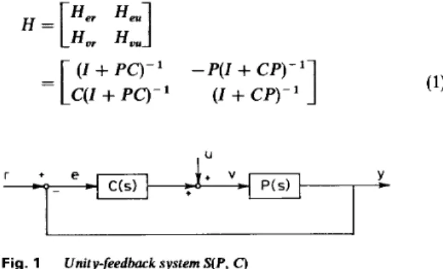
Consider the unity-feedback system S(P, C) shown in Fig. 1, where P(s) E Rq, &)" x n is the plant, C(s) E Rp(s)" is the controller. It is assumed that the dynamical system described by P(s) and C(s) contains no unstable hidden modes. The closed-loop transfer matrix H(s) E Rp(s)2n 2 n from [rT

u q T

to [eT

uTIT

is given by

H =

[$:

:I]

1

( I

+

P c ) - ' -P(I

+

U)-' ( I

+

U - '

=[

C(I

+

PO -' Y +

Fig. 1 Unity-feedback system S(P, C )

The system S(P, C ) is said to be (interally) stable if and only if H E Szn Zn.

In design, in addition to closed-loop stability, it is of interest to make the sensitivity function

11

Her(jw)II small over a certain frequency bandwidth, so that the closed- loop system has good transient response and has good disturbance attenuation. For example, it may be desirable to choose C(s) to make IIH&o)ll

<

E for o E [ - w B , OB], where E > 0 is a small number and oB is the frequency

bandwidth of interest. It is well known [4] that the right- half-plane transmission zeros of the plant limit the achievable lower bound of the sensitivity function. Zames and Bensoussan [ l l ] show that, if the plant is minimum phase, the sensitivity function can be made arbitrarily small over any specified bandwidth while satisfying a pre- scribed bound at all other frequencies by a controller of the following form:

where y > 0, m > 0, 1 > 0,

k

E N, and V(s) is in the form of a modified plant inverse. In the following, we give cri- teria for constructing V(s) and selecting y, m, 1, and

k.

Given that P(s) E 88,. &)" x n is nonsingular and

minimum phase, write

where N(s) E R[s]" and a(s) is the monic least common denominator of the entries of P(s), a+(s) and a-(s) are monic and only have zeros in C + and C - , respectively. Assume that pl,

. . .

, pk are the zeros of a+($ and let b E N

be the smallest integer such that

b > m a x { l p l I , . . . ? lpkl} (4) and let V(s)-' := N(s)/(a+(s

+

b)a-(s)). It is easy to see that V(s)-' has no pole in C +

.

Since

( 5 ) V ( S ) = U + ( S

+

b)a-(s)N(s)-'

we have

Consider the controller C(s) defined by

C(s) = V(s)D(s) = V(s) diag [dl(s)

.

* * d,(s)] ₍₇₎

where V(s) is given by eqn. 5 and

di = y i(

A

s + m i

)

(

Ly

s + l i

yi > 0, mi > 0, li > 0, i = 1, 2,

.. .,

n, and

k

is the largest relative degree of entries of V(s). Note that the controller C(s) defined in eqn. 7 is strictly proper and that the 1/0 map H,, = PC(1

+

PC)-' is diagonal.

The following theorem gives conditions on m i , yi, and l i , i = 1, 2,

...,

n, so that the closed-loop system S(P, C) is stable and satisfies prespecified sensitivity bound in each channel.

Theorem I

Suppose P(s) E Rp, o(s)" is nonsingular and minimum phase. Let b satisfy eqn. 4 and let V(s) and g(s) be as defined in eqns. 3, 5, and 6. Suppose, for i = 1, 2,

. ..

, n, 0 <

<

1, Mi > 1, oBi > 0, and 0 < hi < (1 - M ; ' ) are given. Under these conditions, if, for i = 1,2,

. . .

,

n,

( M l ) mi max {wBi, b} and satisfies sup lg(mie-@) - 11

<

1 - hi 101 C n / 2 and sup Ig(jo) - 1 I

<

1 - M;' -

ai

lolami

(M2)

yi > 0 and satisfies where and (9)

there exists Ii > 0 large enough, i = 1, 2, ..., n, such that with the controller C(s) defined by eqns. 7 and 8:

(i) the system S(P, C) is stable;

(ii) the sensitivity matrix ( I

+

PC)-' is diagonal; and (iii) for i = 1,2, . . . , n,

Comments :

(i) Since limR+m suplsl

I

g(s) - 1 I = 0, the mis in ( M l ) exist.

(ii) Since g(s) has no zeros in C + ,

lli

> 0,

52i

> 0, and thus y i exists, for i = 1 , 2 , .

. .

, n.

(iii) In general, mi and yi increase with decreasing values of M i and respectively.

(iv) It follows from the theorem that the design for each channel can be carried out separately.

In design, m i , yi and

li

are tuned sequentially to achieve the prespecified sensitivity bound in each channel. Proof: See Appendix 10.

3

Consider the unity-feedback system S(P, C) shown in Fig. 1, where the external signal r(t) = [rl(t),

...,

r i t ) ,

...,

Decoupling design for periodic inputs

I E E PROCEEDINGS-D, Vol. 139, NO. I , J A N U A R Y 1992 2

r,,(t)lT is piecewise continuous and for i = 1, 2,

. . . ,

n, ri(t) is &-periodic with Fourier series expansion :

where cik E _{C and} > 0. It is well known [9] that is r i t ) and its first 1 - 1 derivatives are continuous, then

I

c i k

I

-+ 0 as k --t CO at least as rapidly as h/k'+', where h is a constant independent of k. Suppose that the ith channel input ri(t) has most its power concentrated in its first qi harmonics, then, in design, it may be sufficient to track these qi harmonics at steady-state while keeping the amplification at the frequencies beyond 2nqi/T, within a prespecified bound.

In order for the unity-feedback system S(P, C) to track q-periodic input, i = 1, 2, ..., n, with small tracking error, let considers the controller

C(S) = V(S)D(S)F(S) (14)

where V(s)D(s) is defined in eqn. 7, oi = 2471, i = 1, 2,

. .

, , n, and

F(s) = diag

Cfl(4

. . .

fh)l

s

+

1 4 1 (s

+

k w J 2

= diag

[T

n

k = l S 2

+

k 2 W :

Note that the only difference between the controller defined in eqn. 14 and that defined in eqn. 7 is the diag- onal F(s) which is added to provide tracking of the first qi harmonics of the T-periodic input in the ith channel. In design, the number qi will be determined by the steady- state tracking error requirement. The following corollary, which follows directly from theorem 1, gives conditions on D(s) so that the controller C(s) yields the stable closed- loop system S ( P , C ) with decoupled sensitivity matrix and achieves prespecified bounds on the sensitivity function.

Corollary

I

Suppose P(s) E R,, &)"

'"

is nonsingular and minimum phase. Let b satisfy eqn. 4 and let V ( s ) and g(s) be as defined in eqns. 3, 5, and 6. Suppose, for i = 1, 2,

..., n,

0 <

<

1, M i > 1, oBi > 0, and 0 < di < (1 - M i ' ) are

given. Let J@), i = 1, 2,

. .

.

, n, be as defined in eqn. 15. Under these conditions, if, for i = 1,2,

. . .

, n,

mi 2 max { o B i , qi a i , b } and satisfies'

(ml) lei Q 4 2 sup

I d . ( m i e j e )

-

1

I

<

1 - di and sup I g f , ( j o ) - 11

<

1 - M;' - di lwlbmi (G2) y i > 0 and satisfies where

Use sfls) to denote g(s)f,(s) for simplicity.

I E E PROCEEDINGS-D, Vol. 139, N O . I , J A N U A R Y 1992

there exists li > 0 large enough, i = 1, 2, . . . , n, such that with the controller C(s) defined by eqns. 14 and 15:

(i) the system S ( P , C ) is stable

(ii) the sensitivity matrix ( I

+

PC)-

'

is diagonal and (iii) for i = 1, 2, .

.

. , n,

and

(b) (I

+

PC); ' ( j k q ) = 0

k

= 0, f 1, k 2 ,

...,

kqi (20) Comments:

(i) Note that, since ( I

+

PC),;'(jkoi) = 0, k = 0, f 1,

f 2,

. . .

, f q i , the system tracks any q-periodic input which contains only the first qi harmonics (in addition to the DC component) in the ith channel.

(ii) The parameters m i , y i , and Ii can be tuned indepen- dently for each channel to achieve prespecified sensitivity bound.

(iii) In design, the number qi is determined by a pre- scribed relative steady-state tracking error.

4 Time-domain steady-state error analysis We analyse the time-domain steady-state performance of the system S(P, C ) with the controller C(s) prescribed in corollary 1. Assuming that the input r(t) is known, we will derive an upper bound on relative steady-state tracking error in each channel. Since the system S(P, C) is decoupled, it suffices to analyse just one channel. To sim- plify notations, we assume in this section that the signals e(t), y(t), u(t), r(t) in Fig. 1 are all scalar functions and hence the plant and the controller are SISO. Let y,(t) be the steady-state output function due to the T-periodic input r(t) with u(t) = 0 (see Fig. 1)'. Let ess(t):= r(t)

- y,,(t). Note that ess(t) is the steady-state tracking error. Since S(P, C) is linear time-invariant and stable, e,,(t) is also periodic.

Define the relative steady-state tracking error of the system S ( P , C) where f T f T d = e,2,(t) dt and 9 =

J

r2(t) dt 0 0 Let r ( t ) =

CF=

- sentation of r(t). Define

ck ej21rnfiT be the Fourier series repre-

N

r N ( t ) = ~ ~ e j ~ ~ ~ ~ ' ~

k = - N

and

.!?N =

s:(.(l)

- rN(t)}2 dt

Note that rN(t) is the sum of the first N

+

1 harmonics contained in r(t). With these definitions, we are ready to state the following theorem which gives an upper bound on %.

We note that, although the input U has the interpretation of plant

input disturbance, the inclusion of U in Fig. 1 is mainly to allow the determination of closed-loop internal stability [lo] through the stability of transfer matrix H in eqn. 1.

Theorem 2

Consider the stable system S(P, C ) with T-periodic input r(t) and u(t) = 0. Assume the sensitivity function satisfies

and

(1

+

P C ) - ' ( j k w 0 ) = 0 k = 0, +1, f 2 ,

...,

+ q (25) where w o = 2 n / T . Let Q E N be such that Q

<

oB/o0 <

Q

+

1. Let '93 be as defined in eqn. 21. Under these condi- tions, (26) (27) 9 9 (ii) '% d E'

$

+

(M'

-

E') (i) ' % < M 2 9 i f Q d q 9 9 9 if Q > q

The following lemma, which is used in the proof of theorem 2, follows directly from Parseval's theorem [SI.

Lemma I

For 9, defined in eqn. 23, we have

m and N P N = 9 - T

1

IckI2 k = - N (29) Proof of theorem 2

Let

4(s)

:= (1

+

P C ) - '(s). The steady-state tracking error

m e,,(t) =

2

(1

+

PC(jkwo))-lckejk"O' k = - m m = 4(jkWo)ckejkoot k = - m Since 4(jkw,) = O k = 0 , f l , f 2 ,

...,

f q thus W

e,,(t) =

C

(4(jkoo)ck ejkuot

+

4(

-jkoo)c? e - j k w o z ) ( 4 ( j & o o ) c k ejkwot

+

@(jkw,)*c: e-jkoot)

k = q + l

m

=

k = q + 1

From the orthonormal property,

8 = [e:&) dt

=

6'

{

k$+ l(ck 4(jko0Pk"O'

+

c: 4(jko0)*e-jk"Ot)

it follows from eqn. 30 that m

d

<

2TM2

1

1ck12

k = q + l

Thus, from eqn. 28, we obtain

d M 2 P q and eqn. 26 follows.

(ii) If Q > q, then

it follows from eqn. 30 that

Q

1

Id(jkwO)1'1ck1'

k - q + l

0 6)

Thus, from eqn. 28, we obtain

E

<

E'[B, - P Q ]

+

~ ~= E'P, 8

+

,(M' - e 2 ) P Q and eqn. 27 follows.

Based on corollary 1 and theorem 2, we give an algo- rithm for the design of decoupling controllers for linear multivariable system with periodic inputs to satisfy pre- specified bounds on relative steady-state tracking error and sensitivity function.

5 Design algorithm

Consider again the system S(P, C ) with u(t) = 0, and suppose the T-periodic input r i t ) , i = 1, 2,

...,

n, are given. Assume that P(s) E Rp, ,,(s)"

"

is nonsingular and minimum phase, and that the numbers

vi

> 0,O < ci d 1,

M i > 1, and wBi > 0 are given. Our goal is to find the controller C(s) defined in eqn. 14 such that

(i) S(P, C ) is stable (ii) ( I

+

P C ) - is diagonal

(iii) the sensitivity function satisfies

(iv) the relative steady-state tracking error specification satisfies

i = 1,2,

...,

n

We propose, in the following, a design algorithm to achieve this goal.

Algorithm 1

Data: 0 < ei d 1, M i > 1, oBi > 0,

v i

> 0, mi = 2 n / T , and 0

< a i

< (1 - M;'),for i = 1, 2,

...,

n.

Step 0: Set i = 1.

Step 1: Determine the harmonic number qi such that

1 Find Qi E N such that Qi d wBi/wi < Q i

+

1.

2 Compute the Fourier coefficients cik of ri(t).

3 Compute PQi from eqn. 29 and use eqn. 26 or 27 to

Step 2: Determine V(s),f;.(s), g(s), and k.

'93i d

vi.

determine qi such that !Xi

< v i .

1 From eqns. 5 and 15, determine V(s) andfi(s) respec-

2 Obtain k and g(s) from V ( s ) snd P(s). tively.

Step 3:

Determine

mi.

10 O I I

-

_m - 1 0 - -81 I I I I I I I 1 0 1 2 3 4 5 6 7 8 time,s

Fig. 4 Plot of tracking error e l ( [ ) 1 Let m , , = max {aBi, q i o i , b).

2 Choose m2i so that

I E l f @ ~ ~ ~ d ~ )

- 1 I d 1 -

ai

for 3 Choose m3, so that 1 Elf{jo)

-

1 I

<

1

-

M ; -

ai

for 4 Let mi = max { m , , , m 2 i , mji}.

Step 4 : Determine y i . Compute

tii

= inf

I Elftk4I

8 E

CO,

421.

E [mji, 00)-

0 E 10, mil

and

12i

= inf Isf,(mieje)I

e E 10, ~ 2 1

IEE PROCEEDINGS-D, Vol. 139, NO. I , J A N U A R Y 1992

and let

Step 5: Determine I , . Choose li > m,/(2'Ik - 1) such that the poles of (1

+

g d , f i ) - ' ( s ) E C - , which then guar-

antee that (1

+

gd,f,)-' E S a n d 1(1

+

g d i f i ) - ' ( j o ) l

<

E , V l o l d osi (3 1) 0.015 -00151 I 0 1 2 3 4 5 6 7 8 time, s Fig. 5 Plot oftracking error e,(t)

If

I(1

+

g d i f i ) - ' ( j o ) I d M i

V l o l

> o s i (32) then go to step 6; else increase li until eqn. 32 holds.

Step 6 : If i = n, then stop; else i = i

+

1, go to step 1 Comments :

(i) The controller is given by C(s) = V(s)D(s)F(s). (iij In genera1,i mi and y i increase with decreasing values M i and c i , respectively.

(iii) li determination plays an important role in this algorithm to satisfy eqn. 31 and 32. Also, from the proof of theorem 1 (see Appendix lo), Ii must be greater than m,/(2'Ik - 1) at least.

(iv) In practical design, m 2 i , m 3 i ,

t l i ,

and

52i

can be determined by a few magnitude plot of the respective functions. For example, to determine

tli

and

5 2 i ,

we only have to plot the magnitude

I

d ( j o )

I

for 0

<

o d mi and the magnitude

I

gf(mi e'e)

I

for 0

<

8 d 7c/2 respectively.

6 Illustrative example The plant is

P(s) = s(s

+

4)(s - 3)

["i

sY36] The periodic inputs are

t - 2t2 0 d t d 1 / 2 2t2 - 5t

+

5 1/2

<

t

<

1

i

rAt) = and O d t G l t 2 - 3 t + 2 l d t d 2 r 2 M = 5

In addition to achieving closed-loop stability, the design is required to satisfy the following specifications3

(i) ( I

+

PC)-' is diagonal

(ii) 'illl

<

0.05% and 'ill, 6 O.OOOl% (33) (iii) 20 log,,

I

( I

+

PC);,'(jw)

I

(34)

-20dB 6 25

'{

8 d B ' d ) o l > 2 5 and

(iv) 20 loglo

I ( I

+

pC);,'(jo)

I

(35)

= 25, o1 = 2n, v 1 = 5 x 10-4, = 0.1, M , =

-20dB V ' ) w l 6 4 5

4

10dB V l w l > 4 5 The following values are given:

2.5, and 6, = &,(l - M ; I ) = 0.006.

(b) oB2 = 45, 02 = 71, 112 = ~2 = 0.1, M 2 = 3.16,

and 6, = &(l - M y ') = 0.0067.

By computations, q 1 = 1, q , = 3, Q1 = 3, and Q 2 = 14 satisfy eqn. 33. Let b = 4,

( a )

V ( s ) = ( s + 1Xs+4)'[++6

3

]

and k = 2

( s + 2 N s + 3) -4 s - 1

Since the plant already has a pole at s = 0, choose

where

and

(s

+

.)2 (s

+

2742 (s

+

37c)2

f 2 ( s ) = ~

-

~

s2

+

72

s2

+

472 s2

+

971,

By steps 3 and 4, it is determined that m , = 28, m2 = 50,

t I 1

= 1.2,

5,'

= 1.15, y , = 20,

t I 2

= 1.1,

522

= 1, and y 2 = 20. By step 5, I , = 650 and l 2 = 1100 satisfy eqns. 34 and 35, respectively. The controller is given by C(s) = V(s)D(s)F(s), where 28 650' D(s) = diag 20

[

-

s

+

28 (s

+

650)' 20

-

s

+

50 50 (s

+

11002 1100)2

1

It is easy to check that ( I

+

PC)-' is diagonal. The plots of the sensitivity function

1

( I

+

PC);'(jw)

I

and the track- ing error ei(t), i = 1, 2, are given from Figs. 2 to 5. For comparison, the sensitivity function and tracking error corresponding to the controller C(s) = V(s)D(s) without frequency modes are also plotted. By computation, 'ill, = 4.8 x I O p 4 and 'ill2 = 9.3 x I O p 7 . Thus eqn. 33 is satis- fied. It can be seen from Figs. 2 and 3 that sensitivity functions satisfy eqns. 34 and 35, respectively. Note that the upper bounds are almost reached at w z 500 rad/s and w % 800 rad/s, respectively. Figs. 4 and 5 show that

the tracking errors decrease considerably by the intro- duction of frequency modes F(s).

7 Conclusion

We propose an algorithm for the design of controller for linear multivariable minimum phase plants with periodic

Specifications on disturbance attenuation and transient response are reflected in the bounds of the sensitivity functions.

inputs. The periodic inputs may have different periods in different input channels. The controller designed yields stable closed-loop system and decoupled sensitivity trans- fer matrix. Other design specifications include an upper bound on the relative steady-state tracking error and an prescribed bound on the sensitivity function in each channel. The design method is a practical alternative to the so-called repetitive controller. Interesting topics for further study include the extension of this result to non- minimum phase plants and the effect of robustness requirement on the achievable time-domain and frequency-domain specifications.

8 Acknowledgments

This research was sponsored by the National Science Council of ROC under grant NSC-79-0404-E009-07. The authors wish to thank the reviewers whose comments improve the clarity of this paper.

9 1 2 3 4 5 6 7 8 9 References

BAK, J., and NEWMAN, D.J.: 'Complex analysis' (Springer-Verlag, DAVISON, E.J., and PATEL, P.: 'Application of the robust servo- mechanism controller to systems with periodic tracking/disturbance signals', Int. J. Control, 1988,47, (I), pp. 11 1- I27

FRANCIS, B.A., and WONHAM, W.M.: 'The internal model prin- ciple for linear multivariable regulator', Appl. Math. Opt., 1975, 2,

pp. 17&194

FRANCIS, B.A.: 'A course in H, Control theory' (Springer-Verlag, 1987), pp. 134140

HARA, S., and YAMAMOTO, Y.: 'Stability of repetitive control system', Proc. 24th Con& Decision Contr., 1985, pp. 326-327 HARA, S., and NAKANO, M.: 'Synthesis of repetitive control system and its application', Proc. 24th Conf. Decision Contr., 1985, pp. 1384-1392

HARA, S., and YAMAMOTO, Y.: 'A new type servo system for

periodic exogenous signal', IEEE Trans., 1988, AC-33, (7), pp. RUDIN, W.: 'Principles of mathematical analysis' (McGraw-Hill, 1976), pp. 191-192

TOLSTOV. G.P.: 'Fourier seriers' (Prentice-Hall. 19621. DD. 13C131 1982), pp. 71-72

659-668

10 VIDYASAGAR, M.: 'Control system synthesis: a"fH;ltorization approach' (M.I.T. Press, 1985), pp. 99-100

11 ZAMES, G., and BENSOUSSAN, D.: 'Multivariable feedback, sensitivity, and decentralized control', IEEE Trans., 1983, AC-28, (ll), pp. 103C1035

10 Appendix Proof of theorem 1

We define R[p, r):= {s E ClRe(s) > 0, p 6 1st < I } ; O[p,

r ] := The boundary of R(p, r). Let

i = 1, 2, ..., n

Gi

= (1

+

gdi)-' we have ( I

+

PC)-' = diag [(l

+

g d J ' ... (1

+

gd,,)-'] = diag [$1

. . .

$,,I

We shall prove I $ i j o ) I 6 E i , v l w l 6 o s i ;

(a) for i = 1, 2,

. .

. , n, $is) is bounded in Q [ O , OBi] and

(b) for i = 1,2,

. . .

, n, Icli(s) is bounded in R(oBi, 00) and

I

$Lie)

I

<

Mi,

v

10 I

> OB,; and

To prove (a), note that if

( e ) H ( s ) E S2" 2 n .

then

then 1 3 1 + - Ei (37)

I

$ i ( @ )

I

<

Ei

v

I I

<

o ~ i

Thus (a) holds if eqns. 36 and 37 are true. We now show that eqns. 36 and 37 are true, provided that Ii is large enough. Since

I

mJ(mi

+

j o )

I

2 1/J(2), V I w

I

<

mi and

I

zi/(li + j w )

If

2 1/J(2),

v

I O I

<

liJ(2'Ik - 1) if Ii 2

mJ/(2'Ik

- l), then

Similarly, since

I

mi/(s

+

mi)

I

>, mJ(

I

s

I

+

mi) 2 1/2, Vs E

QCo,

mil

and

I

lJ(s

+

Zi)

Ik

2 I!/(

I s

I

+

l i r 2 1/2, Vs E

n[O,

Ii(2'Ik - l)] if

li

>

mi/(2'Ik - l), then

(39)

Thus, if Zi 2 mJ(21'k - l), then eqns. 38 and 39 hold.

modulus principle [ 13 Vs E Q[O, mi],

Since g(s)-' is analytic in

C+

, thus by the maximum

lg(s)lr1 = lg(s)-ll

<

sup lg(s)-ll

s E W O , mi] 1

s E W O , mi]

It follows from eqn. 40 that Vs E nC0, mi},

I d s ) I

2 inf Ig(s)l = m i n

{tli?

tzi}

(41)

s E e [ o , mi]

where

tli

and

tZi

are defined in eqn. 11.

Note that

rli

> 0 and

tZi

> 0, since all the zeros of

g(s) E

C -

.

Since 2tLi1(1

+

(1/q)) 2 45,' and y i satisfies eqn. 10, thus

and V o E [ -m i , mi],

1 2 1 + -

Ei

Since mi 2 os. thus eqns. 36 and 37 are true, provided that Ii 2 mi/(2*Ik - 1). To prove (b), let J J s ) := nJ(s

+

ni), ZEE PROCEEDINGS-D, Vol. 139, NO. 1, J A N U A R Y 1992

d i s ) = yi - - = yiJmi(s)J;(s)

s + m ,

mi

(

S + I i Ii

>'

(43) From eqn. 44, if SUP

I

Ai(s)

I

=

p i

< 1 (45) s E n ( m i , m) then I$i(s)I<I1 + A i ( s ) I - ' < ( l - p i ) - ' V S E R ( ~ , ~ ) Similarly, if (46) 1 sup lAi(jo)l

<

1 - - 101 > m i M i then I$i(jw)l

<

I1

+

Ai(jo)I-'

<

M i

V l o l

> mi

We show that eqns. 45 and 46 are true, provided Ii is Thus (b) holds if eqns. 45 and 46 are true.

Since g(s) is proper and m i 2 b,

I

g(s)I is bounded in

n(q,

00). Also,

I

J ~ ~ ( ~ ~ + ')(s)

I I

J:,i(s) - 1

I

+ 0 uniformly in

n(q

, 00)

as

loi

+ 01) (48)

where

loi

belongs to positive integers; thus, given any cOi > 0, there exists

li

2

loi

> 0 such that

I

Ais)

I I

ds) - 1 I

+

coi VS E

n(q,

00) (49)

I

g(s) - 1 I

<

1

-

ai

vs E

n(q,

CO)

I

g ( j o ) - 1

I

<

1 - M i '

-

J i

Since m i satisfies eqn. 9, we get

and

V I

0 1

> mi

8

Therefore, if we choose cOi =

ai,

then there exists

li

3 IOi 2 ~ n i / ( 2 ' / ~

-

1) large enough such that eqns. 45 and 46 are true.

Finally, we show that H(s) belong to Sz"

"

'".

Since P(s) and C(s) are strictly

proper,

thus

H(s)

belongs to Rp(s)ZnX2n. We have shown that (I

+

PC)-' E S""", By assumption, P(s)-' is analytic in

C,;

By construction, C(s)-' is analytic in

C,

.

Thus P(I

+

U ) - '

=(I -(I

+

Pc)-')c-'

E P X "

( I

+

cq-1 = P - ' P ( I

+

c P ) - ' E S""" and

C(I

+

Pc)-' = ( I - ( I

+

cP)-')P-' E S"""