小型開放經濟體系下金融中介對景氣循環之影響 : 東亞四國之實證研究

全文

(1)Dynamic Effects of Financial Intermediation over the Business Cycles in Small Open Economies - Empirical Studies on Four East Asian Countries. Shu-Hua Chang1 and Bi-Juan Lee2. This paper provides empirical evidence that the financial intermediation disturbances can generate business cycles in small open economies. We extend the framework of Lehr and Wang (2000) to a small open economy and apply the Structural VAR technique pioneered by Blanchard and Quah (1989) in order to reexamine the role of “financial intermediation” shocks on business cycles on the four Asian countries: Taiwan, Japan, Korea, and Singapore. The results indicate that financial intermediate shocks can play a significant role in explaining business cycle fluctuations of these four Asian countries. We also find that the dynamic responses of output to financial intermediation shocks display similar patterns in all cases across countries; however, the magnitude of the one-standard-deviation financial intermediation shock completely differs. Further, the historical decompositions support the ability of our empirical model to recover the structural financial intermediation disturbance accurately. These findings are also consistent with those from Lehr and Wang (2000) and Chang and Wang (2003). The only difference from Chang and Wang (2003), in particular, is that the magnitude of output response to financial intermediation shocks is relatively large in Taiwan and Singapore and much smaller in Japan and Korea.. Key words: financial intermediation, business cycle, structural vector autoregressive model, small open economy 1. Shu-Hua Chang is the Associate Professor in Graduate Institute of Finance and Economics, Aletheia University, Tamsui. 2 Bi-Juan Lee is a graduate student in Graduate Institute of Finance and Economics, Aletheia University, Tamsui. 1 第五屆全國實證經濟學論文研討會 The 5th Annual Conference of Taiwan's Economic Empirics.

(2) 1. Introduction Ever since the pioneering contributions of Schumpeter (1911), and earlier recently Goldsmith (1969), McKinnon (1973) and Shaw (1973) the relationship between financial development and real activities has been extensively studied. Schumpeter (1911) emphasized the importance of the banking system in economic growth and highlighted financial institutions can actively spur innovation and future growth by identifying and funding productive investments. Goldsmith (1969) suggested that the degree of financial development is measured by the value of financial intermediary assets divided by GNP. McKinnon (1973) and Shaw (1973) showed that the state of development of financial markets is typically determined by legislation and government regulation, in their terminology, the degree of financial repression. This “financial repression” is caused by distortions of various sorts - the interest rate ceilings, high reserve requirements and directed credit programs - which result from government restrictions and reduce economic growth. Furthermore, growing theoretical literatures discuss the channel through which financial intermediation affects the economic growth. From the early 1980s on, most of the studies on the interaction between finance and real economic variables are particularly concerned with informational asymmetries as determinants of the behavior of financial markets and institutions. Information acquisition costs create incentives for financial intermediaries to emerge (Diamond 1984; Boy and Prescott 1986). They modeled the critical role that banks play in easing information frictions and therefore in improving resource allocation. In their works, asymmetric information and costly monitoring imply that financial intermediation emerges as the dominant vehicle for carrying out borrowing and lending. Greenwood and Jovanoic (1990), Bencivenga and Smith (1991), and King and Levine (1993b) have carefully documented the links between financial intermediaries and economic activity. As the financial system develops, households substitute out the unproductive assets, raising the total supply of credit, the quantity and quality of investment, and hence faster economic growth, the rate of capital accumulation, and improved efficiency of capital allocation. These studies highlight the positive role of banks in acquiring information about firms and managers and thereby improving resource allocation. In addition, they suggest that, by providing the services to the economy, financial intermediaries influence savings and allocation decisions in ways that may alter long-run growth rates. However, some economists believe that finance is a relatively unimportant factor in economic development. For example, Lucas (1988) terms the financial factors “over-stressed.” In other model, Bencivenga et al. (1995) notes that financial 2 第五屆全國實證經濟學論文研討會 The 5th Annual Conference of Taiwan's Economic Empirics.

(3) development can hurt economic growth. Specifically, higher return from better resource allocation may depress saving rates enough such that overall growth rates actually slowly with enhanced financial development. King and Levine (1993b) also found that government intervention in the financial system has a negative effect on the growth rate. Since a lot of literature had confirmed that finance is an essential factor for growth, and a body of work makes this issue clear, it is now well known that financial development is crucial for economic growth. Early studies have large contributions on the link between financial intermediation and economic growth. But, they largely ignored the influence of financial intermediary development on business cycle fluctuations. Therefore, it is interesting to develop an empirical analysis to examine the dynamic effects of financial intermediation over the business cycles; and this study fills this hole. Recently, the approach of long-run structural VAR proposed by Blanchard and Quah (1989) has been widely used to examine output movement driven by the macroeconomic fluctuations. Lehr and Wang (2000) use this approach to estimate the responses of output to the financial intermediation disturbance for United States, United Kingdom, and Germany. Moreover, Chang and Wang (2003) use this method to investigate the effects of financial shocks on business cycles among four East Asian countries-Taiwan, Japan, Korea, and Singapore. These papers, however, both focus on a closed economy. In fact, the financial systems and economic environments of these four Asian countries are similar to small open economies. Besides focusing on the financial intermediations, our paper differs from these two papers by introducing “external/world” shocks into the model; this study is better able to quantify the effects of output to financial intermediation shocks in a more completed system. The purpose of this paper is to extend the framework of Lehr and Wang (2000) and the long-run structural VAR method to a small open economy in order to reexamine the role of “financial intermediation” shocks on business cycles on the four Asian countries: Taiwan, Japan, Korea, and Singapore. Thus, we employ foreign, domestic variables, three financial indicators, and new data to give an insight into this issue. More specifically, in addition to fiscal, technological, monetary, and three alterative indicators of financial intermediations, we also concern the world interest rate to extend the models as a framework of small open economy. The remainder of this paper is organized as follows. Section 2 introduces the econometric methodology. In Section 3, we describe the data and present the main results; we also examine the sensitivity of the results to alternative identifications. Section 4 draws some conclusions.. 3 第五屆全國實證經濟學論文研討會 The 5th Annual Conference of Taiwan's Economic Empirics.

(4) 2. Empirical Methodology In this section, we apply the Structural VAR technique pioneered by Blanchard and Quah (1989) and extend it to include “world/foreign” shocks to study the economic fluctuations in small open economies. In contrast to the simultaneous equation method, this structural VAR approach focuses on the responses of the “observable” endogenous variables to “unobservable” exogenous structural shocks. In other words, the structural VAR procedure recovers the structural shocks from the observed variables. Moreover, this structural VAR method is economic meaningful whereas Sims (1980) VAR approach is “atheoretical.”3 Firstly, we consider a small open economy model that incorporates both foreign and domestic disturbances and financial shocks. Theoretically, a small open economy is attributed to an economy as world price or world interest rate “taker.” That is, the analysis restricts domestic shocks by not allowing them to affect the world variables. Suppose that the economic system is driven by five structural shocks: (i) a world interest rate shock ( ξ tr ), (ii) a domestic fiscal shock ( ξ tg ), (iii) a domestic *. financial shock ( ξ tθ ), (iv) a domestic productivity shock ( ξ ty ), and (v) a domestic monetary shock ( ξ tm ). Because of the unobservable nature of the structural shocks, additional identifying assumptions are necessary to recover the underlying structural shocks from data. According to theoretical arguments, in the long run, four restrictions are used to identify the structural shocks. (Hereafter, for the sake of brevity, unless indicated otherwise, “shock” will refer to a structural shock.) The first two restrictions are that aggregate demand shocks have no long-run effects on output. These restrictions are consistent with an aggregate demand-aggregate supply model with a vertical long-run aggregate supply curve. That is, in our model, the growth rate of government size is exogenous and the money is superneutral in the long run. The third restriction states that financial intermediation is insensitive to output in the long-run. The final restriction, in the essence of small open economy assumption, domestic shocks are not allowed to affect the world variables; this restriction means that the world shock is absolutely exogenous in the long-run. We consider a vector of stationary variables Xt and a vector of structural shocks 3. See Cooly and Leroy (1985) for more details. The VAR method is not economic meaningful, in the sense that there has been no use of economic theory to specify structural equations between various sets of variables. Economic variables tend to move together over time and also to be autocorrelated in VAR system. 4 第五屆全國實證經濟學論文研討會 The 5th Annual Conference of Taiwan's Economic Empirics.

(5) Ut. To extract the five structural shocks, we estimate a five-variable reduced-form VAR for each country, such as: ∞. X t = ∑ AiU t −i = A(L )U t ,. Var (U t ) = I. i =0. where. the. variables. in. the. (1). model. are. denoted. by. ′ ′ RG ⎫ ⎧ * , ∆ ln( FI ), ∆( RGDP), ∆( M 1)⎬ = ∆r * , ∆g , ∆θ , ∆y, ∆m that X t = ⎨∆( RI ), ∆ ln RGDP ⎭ ⎩. {. }. represent the difference of world real interest rate, and the log differences of the government size, financial intermediation, real output, and money supply; ∞. Ai = ∑ Ai Li and Ai ’s are matrices of unknown structural coefficients and the i =0. disturbances are unobservable; A(L) denotes a 5 × 5 matrix of lag polynomials; and. {. U t = ξ tr , ξ tg , ξ tθ , ξ ty , ξ tm *. } denotes. a vector containing the structural shocks with. E[εε ′] = I (the identity matrix);. Eq. (1) assumes that all endogenous variables are integrated of order 1, I (1). In addition, the five structural shocks have unit variance and are mutually orthogonal. Secondly, because Xt is stationary, there is a unique Wold-moving average representation: X t = C (L )Vt , Var (Vt ) = Ω, C 0 = I (2) After estimating the vector autoregressive representation of X t , we can then invert the estimated coefficients to obtain C i ’s.4 Next, comparing equations (1) and (2), we can obtain: Vt = A0U t (3) Ai = C i A0 , i = 1,2,K p (4) Since Ci is obtained by inverting the estimated coefficients of VAR system, Ai is solved when A0 is known. In an n-variable model, identification requires n2 restrictions: in our case, n2=25. This can be written out in matrix form as Eq. (5). Following Blanchard-Quah framework, we assume that the structural shocks are orthogonal and have unit variance, i.e. Var (Vt ) = Ω . This gives us (n(n + 1) 2) = 15 restrictions. To sufficiently estimate the dynamics of the system in Eq. (1), we need ten more identifying restrictions on the long-run impacts of the structural shocks. The 10 restrictions are used to solve the Ai matrix.. 4. Assume that the VAR model is Xt=B(L)Xt+Vt, then the moving average representation of Xt is Xt=(I-B(L))-1Vt=C(L)Vt. As (I-B(L))C(L)=I, the Ci will be known when Bi is estimated by the VAR model in the usual way. 5 第五屆全國實證經濟學論文研討會 The 5th Annual Conference of Taiwan's Economic Empirics.

(6) ⎡ a11 ⎢a ∞ ⎢ 21 Ai = A( L) = {aij } = ⎢ a31 ∑ ⎢ i =0 ⎢a 41 ⎢⎣ a51. a12 a 22. a13 a 23. a14 a 24. a32. a 33. a34. a 42. a 43. a 44. a52. a 53. a54. a15 ⎤ a 25 ⎥⎥ a35 ⎥ ⎥ a 45 ⎥ a55 ⎥⎦. (5). Extending Lehr and Wang (2000), we assume that (i) domestic shocks do not affect the world variables, (ii) the government size is given exogenously, (iii) financial intermediation is insensitive to output shocks, (iv) the monetary shock has no long-run effect on output movement. Due to these identifying restrictions, the Ai matrix is a lower triangular matrix, i.e., a12=a13=a14=a15=a23=a24=a25=a34=a35=a45=0, as shown in Eq. (6). It is also a just identified representation of the system in Eq. (1). ⎡∆r * ⎤ ⎡ a11 ⎥ ⎢ ⎢ ⎢ ∆g ⎥ ⎢a 21 X t = ⎢ ∆θ ⎥ = ⎢ a31 ⎥ ⎢ ⎢ ⎢ ∆y ⎥ ⎢a 41 ⎢ ∆m ⎥ ⎢⎣ a51 ⎦ ⎣. 0 a 22 a32 a 42. 0 0 a33 a 43. 0 0 0 a 44. a52. a53. a54. ⎤ ⎡ξ r ⎤ ⎥⎢ g ⎥ ⎥ ⎢ξ ⎥ ⎥⎢ξ θ ⎥ ⎥⎢ y ⎥ ⎥⎢ξ ⎥ a55 ⎥⎦ ⎢⎣ξ m ⎥⎦ 0 0 0 0. *. (6). These restrictions, including those provided by the variance-covariance matrix, can be used to determine the unique Ai matrix. Accordingly, we can get all Ai matrices. Obtaining the matrices of U t and Ai ’s, we can figure out the process of X t from equation (1). Finally, we use the impulse-response functions and variance decompositions to illustrate the dynamic character of the empirical model for each country, as well as the historical decomposition to quantify the importance of financial intermediation to output. There are two potential problems with the interpretation of these financial intermediation shocks. First, it may be that other shocks do have effects in our identifications; our system that is subject to only five structural disturbances may be misleading. In addition to financial intermediation disturbances, in fact, we have included external shock, fiscal, monetary, and real shocks. However, the real shocks may contain supply, persistent demand, and oil price disturbances; there is no obvious omission of any other significant shock in our model. Second, it should be pointed out that the long-run casual ordering of the benchmark model is world real interest rate, government size, financial intermediation, output, and money supply. According to the small open economy assumption, the world variable is most exogenous; based on identifying restrictions consistent with theoretical assumptions, the ordering of government size, output, and money supply is natural and plausible. There may be alternative theoretical orderings in regard to financial intermediation as well as two 6 第五屆全國實證經濟學論文研討會 The 5th Annual Conference of Taiwan's Economic Empirics.

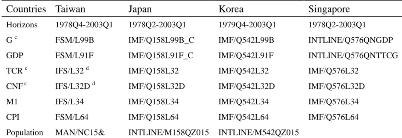
(7) real variables (government size and output), we will leave this ground for our sensitivity analysis to check the robustness.. 3. Empirical results 3.1 The Data In our paper we investigate the time series properties of the business fluctuations on the shock of financial factors for four Asian countries: Taiwan, Japan, Korea, and Singapore with quarterly observations. The sources of our data are summarized in Table 1. We convert these data to real per capita values by using the domestic consumer price index (1995=100) and population over 15 years. 5 The 3-month Treasury-Bill rates of United Stated are as a proxy by the world interest rates. The world interest rates measured in levels, and all the other variables are in logarithms of levels. Our empirical works are performed both by using the EVIEWS version of 4.1 and the RATS version of 5.0. Table 1 Data Sources a, b Countries Taiwan. Japan. Korea. Singapore. Horizons. 1978Q4-2003Q1. 1978Q2-2003Q1. 1979Q4-2003Q1. 1978Q2-2003Q1. Gc. FSM/L99B. IMF/Q158L99B_C. IMF/Q542L99B. INTLINE/Q576QNGDP. GDP. FSM/L91F. IMF/Q158L91F_C. IMF/Q542L91F. INTLINE/Q576QNTTCG. TCR c. IFS/L32 d. IMF/Q158L32. IMF/Q542L32. IMF/Q576L32. IMF/Q158L32D. IMF/Q542L32D. IMF/Q576L32D. CNF. c. IFS/L32D. d. M1. IFS/L34. IMF/Q158L34. IMF/Q542L34. IMF/Q576L34. CPI. FSM/L64. IMF/Q158L64. IMF/Q542L64. IMF/Q576L64. Population. MAN/NC15&. INTLINE/M158QZ015. INTLINE/M542QZ015. Notes: a All the data are extracted from the AREMOS Data Bank of the Ministry of Education in Taiwan. In the table, on the left of slash is the data bank, the right is the retrieval code of the series. b The U.S. 3-month Treasury bill rate is obtained from IMF/M111RIBT3, observations are monthly. Quarterly observations are obtained by averaging over the three months comprising each quarter. U.S. CPI is obtained from IMF/Q111L64. c G: Government Expenditures; TCR: Domestic Credit; CNF: Claims on Private Sector. d Before the second quarter of 1987, the data have been obtained from Financial Statistics Monthly, Taiwan District, the Republic of China (Compiled in Accordance with IFS Format).. Since the focus in our study is the financial activity, we estimate our model by using three alternative measures for financial intermediation derived from banking aggregates. We use three proxies that followed by Goldsmith (1969), McKinnon and 5. Due to the data limitations on availability of quarterly population over 15-year-old of Singapore, we convert theirs to domestic CPI (1995 prices) only. 7 第五屆全國實證經濟學論文研討會 The 5th Annual Conference of Taiwan's Economic Empirics.

(8) Shaw (1973), and King and Levine (1993) to be referred to as Models I, II and III, respectively. Namely, the three financial intermediation measures are (i) the ratio of claims on the non-financial private sector to output, (ii) the ratio of money plus quasi-money to output, and (iii) the ratio of claims on the non-financial private sector to total credit. As we show, in Table 2, we focus on three major dimensions in our small open economy system: foreign, domestic and financial. More specifically, the structural model expressed by including the foreign shock, i.e. world interest rate shock, and domestic shocks such as fiscal, real, and monetary shocks, as well as the financial intermediation shocks. Table 2 Variables and Definitions Measurement. Variables. Definitions. World Interest Rate. R*. The U.S. 3-month Treasury-Bill rates.. Fiscal Policy. GY. The ratio of real government spending to real gross domestic product.. I CNF/RGDP The ratio of claims on the non-financial private sector to output. Financial Intermediation. II. M2/GDP The ratio of money plus quasi-money to output.. III CNF/TCR The ratio of claims on the non-financial private sector to total credit. Real Output. RGDP. Monetary Policy. M1. Real gross domestic product. Real monetary supply.. Notes: 1. In constructing our real interest rates, we assume that inflation follows an AR (p) process: cpit = a( L)cpit −1 + ε pt , where the cpit is U.S. consumer price index in period t, L is the lag p −1 operators, a ( L) = a1 + a 2 L + K + a p L . ε pt are serially uncorrelated disturbances with zero 2 mean and variance σ p . We found that AR (4) minimizes the estimations of both Schwarz Criterion and Akaike Information Criterion. Next, we figure out the expected inflation rates: cpite+1 − cpit cpit . Thereafter, subtracting the expected inflation rate from nominal interest rates, we have the expected world real interest rates. As in Chang and Mao (1997) and Galí (1992), the difference between the nominal interest rate and the one-period-ahead inflation rate serves as a proxy for the real interest rate. 2. GY=（G/CPI）/（GDP/CPI）; TCR= Domestic credit/CPI; CNF= Claims on private sector/CPI.. (. ). From the “output/credit” point of view, Model I captures most directly the production of credit by the banking institutions. This measure isolates credits issued to the private sector, as opposed to credits issued to the public sector, and it also excludes credits issued by the central bank. We believe that it is better to accurately represent the actual volume of funds channeled into the private sector. We interpret this measure as an indication of more financial services and therefore greater financial intermediary development. From the “input/deposits” point of view, Model II represents funds allocated to the banking sector by the public, and is a typical indicator of “financial depth.” The higher the ratio of broad money to GDP implies a 8 第五屆全國實證經濟學論文研討會 The 5th Annual Conference of Taiwan's Economic Empirics.

(9) larger financial sector and therefore greater financial intermediary development. Model III depicts the degree to which banking sectors allocate society’s savings and is a rough measurement of credit allocation. This indicator is designed to measure domestic asset distribution. Although each financial indicator has shortcomings, using this set of indicators provides a richer picture of financial intermediary development than if we used a single measure only. It would strengthen this article to use these three measures that confirmed by previous literatures and to investigate the robustness of our results under various models.. 3.2 Integration and Cointegration Properties of the Data A prior estimation, the data are checked for unit roots and cointegration. Augmented Dickey-Fuller (ADF) and Phillips-Perron (PP) tests for unit roots are computed, and Johansen’s (1990) maximal eigenvalue and trace statistic tests are performed to test for cointegration. 3.2.1 Unit Root Tests To implement the structural VAR, all variables must be in stationary forms. In the presence of non-stationary variables, a related problem is the possibility of finding. spurious regressions.6 We employ the ADF and PP tests to examine the integration properties of the variables. All variables but the world real interest rates are expressed in logarithms. The results indicate that all the variables can be characterized as integrated process with order 1 in each country. 3.2.2 Co-integration Tests Since each time series is integrated of order 1,7 we can then proceed to test for whether any cointegrating relation exists in our five-variable system. When it exists, the dynamic system must be specified as a vector error correction (VEC) model. We applied the multivariate cointegration techniques provided by Johansen and Juselius (1990) and Johansen (1991) to test for cointegration among our variables in four. countries. In addition to the determination of the set of variables to include in the VAR, it is important to determine the appropriate lag length. In order to carry out Johansen’s procedure, we determine the optimal lag length in the simple VAR system first.8 6. See Granger and Newbold (1970). A spurious regression has a high R2, t-statistics that appear to be significant, but the results are without any economic meaning. 7 See Enders (1995). One of the definitions in cointegration is that all variables must be integrated of the same order to be stationary. 8 Our procedure for choosing the optimal lag length was to test from an undifferenced VAR (1) system, increasing the order of VAR by 1 lag until we obtained the minimal Schwartz Information Criterion (SIC). Furthermore, the residuals from the chosen VAR were diagnosed for serial correlation. If the residuals were autocorrelated, we subsequently chose a higher lag structure until they followed serial 9 第五屆全國實證經濟學論文研討會 The 5th Annual Conference of Taiwan's Economic Empirics.

(10) We show the results of the cointegration test which were derived by using the Johansen method in Table 3. Relative to the λtrace test, the λ max test has the sharper alternative hypothesis; as a result, the λ max test is usually preferred for trying to pin down the number of cointegrating vectors (Enders 1995). Therefore, we determined the rank of cointegration for each model by using the maximal eigenvalue test. In our empirical results, all the maximal eigenvalue statistics illustrate the absence of cointegration relationship among variables for each country. The finding of no cointegration implies that there is no long-run equilibrium relationship among all variables over the sample period for these countries. Table 3 Summary of Cointegration Test Optimal Optimal Number of Models Lag Length Case Cointegration Taiwan * R , lnGY, ln(CNF/RGDP), lnY, lnM1 2 2 0 * R , lnGY, ln(M2/GDP), lnY, lnM1 3 2 0 * R , lnGY, ln(CNF/TCR), lnY, lnM1 3 3 0 Japan 2 4 0 R*, lnGY, ln(CNF/RGDP), lnY, lnM1 * R , lnGY, ln(M2/GDP), lnY, lnM1 2 4 0 * R , lnGY, ln(CNF/TCR), lnY, lnM1 2 3 0 Korea 1 3 0 R*, lnGY, ln(CNF/RGDP), lnY, lnM1 * R , lnGY, ln(M2/GDP), lnY, lnM1 2 3 0 * R , lnGY, ln(CNF/TCR), lnY, lnM1 2 3 0 Singapore 1 3 0 R*, lnGY, ln(CNF/RGDP), lnY, lnM1 * R , lnGY, ln(M2/GDP), lnY, lnM1 1 3 0 * R , lnGY, ln(CNF/TCR), lnY, lnM1 1 3 0 Note: R*=U.S. 3-month Treasury-Bill rate, GY= government size, CNF=credit to nonfinancial firms, TCR= total domestic credit; Y= real output; M1= money supply.. For these tests, in brief, each individual series is integrated of order 1, and the empirical evidence fails to support the existence of cointegration relationships among all macroeconomic variables in all countries. Therefore, we can apply the structural VAR model to analyze the dynamic effects of business cycle fluctuations.. 3.3 Impulse Response Functions and Variance Decompositions As refer to the structural VAR specifications, first-differencing translates the log of levels into growth rates and thus allows us to examine the effects of changes in the levels of financial intermediary development on real output. Therefore, we use the uncorrelated process. 10 第五屆全國實證經濟學論文研討會 The 5th Annual Conference of Taiwan's Economic Empirics.

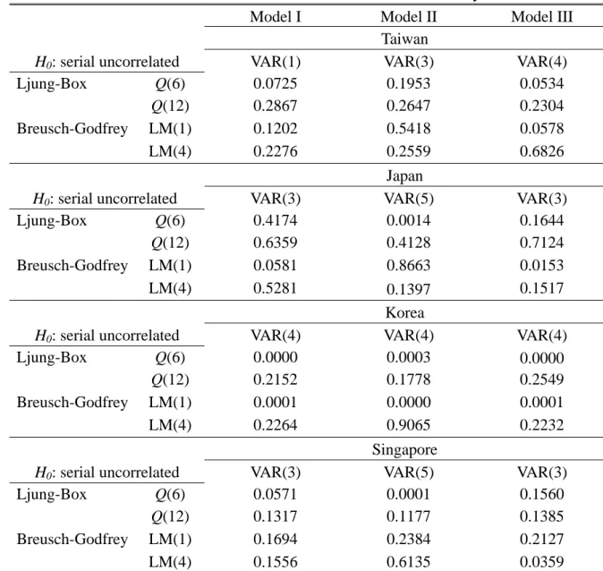
(11) first-difference of the log of levels for each series in the estimation. We also concern the appropriate orders of lag used in the structural VAR framework. Our procedure for choosing the optimal lag length was to test up from a differenced VAR (1) system, and diagnose the residuals from the chosen VAR for white noise process. The residual tests for each system are presented in Table 4. Table 4 Test for Residual Correlation in Structural VAR System Model I Model II Model III Taiwan H0: serial uncorrelated VAR(1) VAR(3) VAR(4) Ljung-Box Q(6) 0.0725 0.1953 0.0534 Q(12) 0.2867 0.2647 0.2304 Breusch-Godfrey LM(1) 0.1202 0.5418 0.0578 LM(4) 0.2276 0.2559 0.6826. H0: serial uncorrelated Ljung-Box Q(6) Q(12) Breusch-Godfrey LM(1) LM(4). VAR(3) 0.4174 0.6359 0.0581 0.5281. H0: serial uncorrelated Ljung-Box Q(6) Q(12) Breusch-Godfrey LM(1) LM(4). VAR(4) 0.0000 0.2152 0.0001 0.2264. Japan VAR(5) 0.0014 0.4128 0.8663 0.1397 Korea VAR(4) 0.0003 0.1778 0.0000 0.9065. VAR(3) 0.0571 0.1317 0.1694 0.1556. Singapore VAR(5) 0.0001 0.1177 0.2384 0.6135. H0: serial uncorrelated Ljung-Box Q(6) Q(12) Breusch-Godfrey LM(1) LM(4). VAR(3) 0.1644 0.7124 0.0153 0.1517 VAR(4) 0.0000 0.2549 0.0001 0.2232 VAR(3) 0.1560 0.1385 0.2127 0.0359. Note: 1. Model I: financial intermediation = nonfinancial credit/output; Model II: financial intermediation = (M2)/output; Model III: financial intermediation = nonfinancial credit/total credit. 2. VAR (.) denotes the optimal order of structural VAR model. 3. Numbers in the table are p-value. Q (6) and Q (12) are the Ljung-Box statistics for sixth- and 12th-order serial correlation in the residuals. LM (1) and LM (4) are the Breusch-Godfrey statistics for first- and fourth-order serial correlation in the residuals.. We calculate Ljung-Box Q statistics at six and 12 lags and Breusch-Godfrey. 11 第五屆全國實證經濟學論文研討會 The 5th Annual Conference of Taiwan's Economic Empirics.

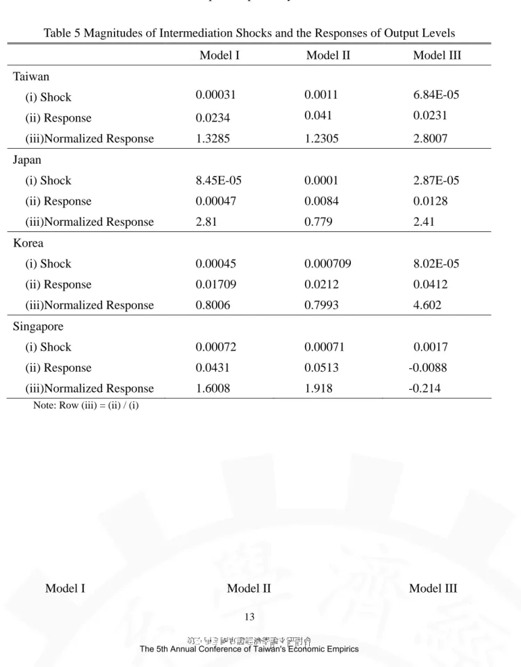
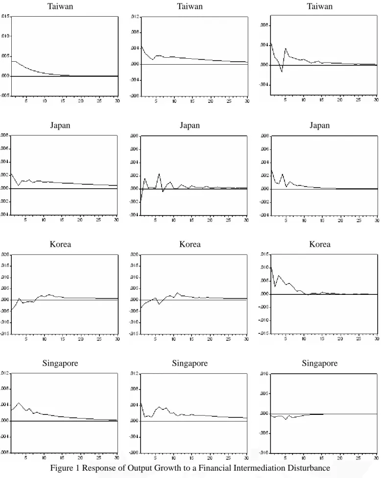
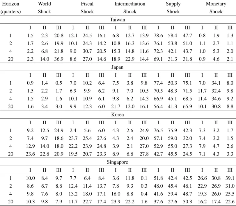
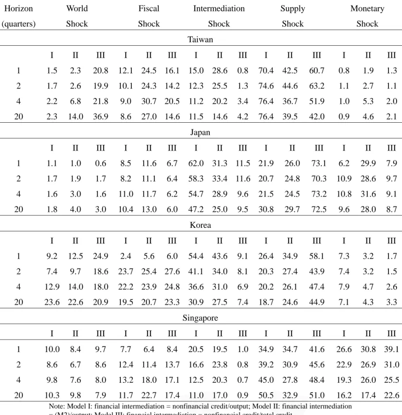
(12) LM (Lagrange Multiplier) statistics at one and four lags for the estimated structural VAR system. Until increasing the order of the VAR by 1 lag could not be rejected by Q statistics and LM statistics, we determine our optimal lag length in the structural VAR model.9 As we can see in Table 6, they are roughly insignificant at the null of serial uncorrelated in the residuals. The normalized accumulated responses of output are listed in Table 5. Comparatively speaking, the one-standard-error shock is relatively small in Japan while it is much larger in Singapore. Taiwan and Singapore have larger normalized magnitude of output response than do Japan and Korea. Some plausible explanations for these differences are discussed below. The size of the one-standard-error shock is larger on the part of Singapore; this is not surprising since Singapore is an offshore financial center of Asian currency market and the offshore banking are often not subject to domestic regulation and can do business in a much less constrained behavior.10 It is presumable that there are much more external and internal financial innovations in this region. On the other hand, the Japanese financial system has always been more developed than those of Taiwan or Korea; as a consequence, we would expect that small innovations in Japan would not cause large effects, whereas small improvements in the other two countries would do. This is also proved to be true in model II and III of these three countries in Table 5. Impulse response functions describe the dynamic characteristics of the empirical model. The impulse responses to each of the structural shocks are shown in Figure 1. In each pattern, it draws the dynamic responses of output growth to a one-standard-deviation financial intermediation shock. The path of output movement is very similarly across countries in response to a financial intermediation disturbance; however, there are variations in their magnitudes. Table 6 reports the results of variance decompositions for output growth due to the five structural disturbances of various steps. This measures the relative contribution of forecast error variance of each shock as a function of forecast horizon. While the impulse-response function reveals the dynamic effects of a one-time shock, the variance decomposition is a convenient measure of the relative importance of such shocks to the system. In Model I, both Taiwan and Singapore attribute a larger role to financial intermediation shocks at four quarters, 15.3% and 16%, respectively, while the results of Japan and Korea indicate little role for financial intermediation in explaining output fluctuations, 9.8% and 3.9%, respectively. In Model II, at the same. 9. The lag length in VAR model will be too short if the residuals are autocorrelated, and it is wise to choose a higher lag structure until they are serial uncorrelated. 10 The Asian currency market is commonly known as the Asian Dollar Market (ADM) because most of the transactions are denominated in U.S. dollars. That is, Asian currency market and Asian Dollar Market are used interchangeably. 12 第五屆全國實證經濟學論文研討會 The 5th Annual Conference of Taiwan's Economic Empirics.

(13) horizon, the results are similar to Model I, financial intermediation shocks in Taiwan and Singapore explain 14.8% and 8.8% of variance, respectively, while there is small portion of variance in Japan and Korea, 6.2% and 2.1%, respectively. The difference appears in Model III, where Korea attributes a much larger role to financial intermediation shocks, 27% at four quarters, while it is much smaller in Singapore, 0.4% at four quarters, in addition, the contribution of intermediation disturbances are 11.6% and 14.3% in Taiwan and Japan, respectively. Table 5 Magnitudes of Intermediation Shocks and the Responses of Output Levels Model I. Model II. Model III. Taiwan (i) Shock. 0.00031. 0.0011. 6.84E-05. (ii) Response. 0.0234. 0.041. 0.0231. (iii)Normalized Response. 1.3285. 1.2305. 2.8007. (i) Shock. 8.45E-05. 0.0001. 2.87E-05. (ii) Response. 0.00047. 0.0084. 0.0128. (iii)Normalized Response. 2.81. 0.779. 2.41. (i) Shock. 0.00045. 0.000709. 8.02E-05. (ii) Response. 0.01709. 0.0212. 0.0412. (iii)Normalized Response. 0.8006. 0.7993. 4.602. (i) Shock. 0.00072. 0.00071. 0.0017. (ii) Response. 0.0431. 0.0513. -0.0088. (iii)Normalized Response. 1.6008. 1.918. -0.2140. Japan. Korea. Singapore. Note: Row (iii) = (ii) / (i). Model I. Model II 13 第五屆全國實證經濟學論文研討會 The 5th Annual Conference of Taiwan's Economic Empirics. Model III.

(14) Taiwan. Taiwan. Taiwan. Japan. Japan. Japan. Korea. Korea. Korea. Singapore. Singapore. Singapore. Figure 1 Response of Output Growth to a Financial Intermediation Disturbance. 14 第五屆全國實證經濟學論文研討會 The 5th Annual Conference of Taiwan's Economic Empirics.

(15) Table 6 Variance Decomposition of Output Growth’s Forecast Error Horizon (quarters). World Shock. Fiscal Shock. Intermediation Shock. Supply Shock. Monetary Shock. Taiwan 1 2 4 20. I. II. 1.5 1.7 2.2 2.3. 2.3 2.6 6.8 14.0. III. I. II. III. I. II. III. I. II. III. I. II. III. 12.7 16.3 14.8 22.9. 13.9 13.6 11.6 14.4. 78.6 76.1 72.3 69.1. 58.4 53.8 42.1 31.3. 47.7 51.0 43.7 31.8. 0.8 1.1 1.0 0.9. 1.9 2.7 5.3 4.6. 1.3 1.1 2.0 2.1. I II III I II 7.5 3.8 9.8 77.4 50.3 9.1 7.0 10.5 70.5 48.3 9.8 6.2 14.3 66.9 45.1 21.7 12.0 16.1 56.4 41.3. III 75.1 71.5 68.5 65.9. I 7.0 11.7 11.4 10.1. II 34.1 32.4 34.6 30.8. III 8.0 9.8 9.2 8.8. 20.8 12.1 24.5 16.1 6.8 19.9 10.1 24.3 14.2 10.8 21.8 9.0 30.7 20.5 15.3 36.9 8.6 27.0 14.6 18.9 Japan. 1 2 4 20. I 0.9 1.5 1.5 1.6. II 1.4 2.2 2.9 3.4. III 0.5 1.7 1.6 3.0. I II 7.0 10.2 6.9 9.9 10.1 10.9 9.9 12.3. III 6.4 6.2 6.1 6.0. Korea 1 2 4 20. I II III I II III 9.2 12.5 24.9 2.4 5.6 6.0 7.4 9.7 18.6 23.7 25.4 27.6 12.9 14.0 18.0 22.2 23.9 24.8 23.6 22.6 20.9 19.5 20.7 23.3. I 4.3 4.3 3.9 6.9. II 2.6 2.4 2.1 6.6. III 24.9 20.0 27.0 27.8. I 76.5 57.1 52.9 42.7. II 75.9 59.0 55.0 45.5. III 42.3 32.0 27.3 24.5. I 7.3 7.4 7.9 7.1. II 3.2 3.2 4.7 4.3. III 1.7 1.5 2.6 3.3. III. I. II. III. I. II. III. 0.1 0.3 0.4 1.6. 51.8 48.0 41.6 37.6. 42.4 45.4 39.4 27.6. 42.5 46.1 48.7 50.3. 26.6 22.9 19.3 16.2. 30.8 26.9 26.0 17.4. 39.1 31.0 25.5 22.6. Singapore 1 2 4 20. I. II. III. 10.0 8.6 9.8 10.3. 8.4 6.7 7.6 9.8. 9.7 8.6 8.0 7.9. I. II. III. I. II. 7.7 6.4 8.4 3.6 11.8 12.4 11.4 13.7 7.8 9.3 13.2 18.0 17.1 16.0 8.8 11.7 22.7 17.4 23.9 22.2. Note: Model I: financial intermediation = nonfinancial credit/output; Model II: financial intermediation = (M2)/output; Model III: financial intermediation = nonfinancial credit/total credit.. Although the empirical investigation above cannot capture the exact channels through which financial intermediation shocks affect the output movement, we still find out some possible country-specific factors for these differences. First of all, development of the financial system in Taiwan definitely contributed to the island’s success by means of stimulating and mobilizing savings as well as allocating investment funds. Thus, the size of financial intermediation’s contribution to the variance of the forecast error is larger in this case than the other three countries, especially for model I (CNF/RGDP) and model II (M2/GDP). It’s worth noting that the portion of (CNF/TCR) in this case is less small than in Japan or Korea. Recall that 15 第五屆全國實證經濟學論文研討會 The 5th Annual Conference of Taiwan's Economic Empirics.

(16) one of the most significant features of the financial system in Taiwan is the “financial dualism,” which means that in addition to the formal (organized, regulated) financial system, there is also an informal (unorganized, unregulated) system that plays a crucial role in financial intermediation. During the period 1964-1990, financial institutions provided the business sector with 55% of its total domestic financing. The informal system accounted for 24%, capital markets 14%, and the money market 7%. Further decomposing the business sector into public enterprises and private enterprises, public enterprises depended primarily on financial institutions as the source of their borrowing, while private enterprises borrowed only slightly more than half from financial institutions and over one-third from informal markets.11 This may have severely distorted resource allocation in view of credit proxy (CNF/TCR) and thus lower its contribution to output movement in Taiwan case. Second, in the financial system of Japan, big businesses and major banks were closely tied by means of a main bank and cross-shareholding relationships. The corporate sector was able to borrow at relatively low interest rates from the banking sector, while small business paid much higher interest rates. During the liberalization process, the financial system underwent a gradual transformation from regulated to deregulated one. An important effect of deregulation on the structure of the financial services industry is the greater presence of security firms in a previously bank-dominated system; and the credits from securities finance companies are heavily dependent on borrowings from banks. This may reduce the effective allocation from banks to the private sectors, such as the little fraction in model I (CNF/RGDP), even in the liability side of model II (M2/GDP). Also, banks in Japan relied heavily on government-led industrial policies, such as government intervention in credit allocation, and spur some largely positive effects on the output fluctuations. As a result, in model III (CNF/TCR) there is larger portion in Japan than in Taiwan or Singapore in explaining the output growth. Third, the results of Korea are obviously similar with the Japan case. Both Korea and Japan relied heavily on government-led industrial policies, however, the passive or subordinate role of Korean banks has led to inefficiency in resource allocation. It is proved that there are fewer portions in model I (CNF/RGDP). Further, the “unhealthy” financial relationship led to the distorted allocation to the banking institutions by Korean government. For this reason, there is less contribution of model II (M2/GDP) to the output fluctuations in Korea case. In addition, Korea has a particular form of bank-enterprise relationship that links each large business group to a particular bank (i.e., the principal transactions bank) closely in the credit control system. In Korea, the government’s control over credit allocation was tightened to 11. For more detailed discussion of Taiwan’s financial system see Patrick and Park (1994). 16 第五屆全國實證經濟學論文研討會 The 5th Annual Conference of Taiwan's Economic Empirics.

(17) keep up with the change in the industrial development strategy toward the promotion of capital–intensive heavy and chemical industry. This may be the reason why the contribution of model III (CNF/TCR) to output fluctuations is the largest in Korea compare to the other three countries. Finally, Singapore is a major financial centre in Southeast Asia; its financial system is dichotomized by separating domestic banking units from the offshore financial center, which is composed of Asian Currency Units (ACUs). Because a financial center consists of a high concentration of financial institutions and underlying markets that allow transactions to take place more efficiently than elsewhere. As such, the high efficiency of resource allocation is shown in both model I (CNF/RGDP) and model II (M2/GDP), in which represents funds allocated to the banking sector by the public. Moreover, the ACU is an offshore banking branch of a domestic bank and deals with nonlocal currency, generally with very little regulation and primarily for nonresidents. Notably, there is less significant relationship between foreign-owned intermediation and domestic output in this financial center. This may cause the inefficiency of domestic credit allocation in the case of Singapore, and this is also testified that the smallest fraction of the variance of forecast errors in model III (CNF/TCR) in contrast to the other countries we studied. In sum, the patterns of dynamic responses of output growth to one-standard-deviation financial intermediation shock are similar to all countries but differ in the magnitude. We find that financial intermediation shocks can be important in explaining fluctuations in small open economies. Moreover, our results support that financial intermediation do influence business cycles in small open economy.. 3.4 Historical Decomposition The historical decomposition allows us quantify the importance of financial intermediation shocks to output fluctuations. For the sake of brevity, we discuss the portion of output movements driven by financial intermediation shocks only, as depicted in Figure 2, and undoubtedly, output will also be influenced by the other four disturbances. In general, independent of the model, the historical decompositions show a similar pattern for each country; as a result, we examine Model I (CNF/RGDP) for each country. The differences are discussed below. In Taiwan, during the second half decade of 1980s, the private sector had accumulated great wealth and the excess of domestic savings over domestic investments, accompanied by a huge surplus and a rapid expansion of the money supply, created a serious excess liquidity. The excess liquidity led to dramatic rises in the prices of stocks and real estate and consequently like generating some spillover effects for banking industry. Further, many private banks have been established in the early 1990s (exactly speaking, the late 1991) creating a competitive situation in the 17 第五屆全國實證經濟學論文研討會 The 5th Annual Conference of Taiwan's Economic Empirics.

(18) banking sector, and as a result it is likely to raise the output during that time. Even since the summer of 1997 when financial crisis broke up in Asia, Taiwan still stood out as a special case; its economic performance remained better than that of the other three countries. In Japan, the financial intermediation shocks have played a positive role in promoting output during 1980-92. In addition, dominated by large institutions, the Japanese banking system has suffered from serious problems since the early 1990s, when the Japanese stock market and urban real estate market both crashed. Delays in responding to these twin asset bubbles made matters worse and led to a banking crisis in late 1997 and early 1998. The combination of these events led into a prolonged downturn in output from early 1990s to the twenty-first century. Also at the start of the twenty-first century, the Japanese financial system is undergoing a major transformation. The Japanese government has begun to reform the Tokyo financial markets by the year 2001 and create a financial centre capable of competing with London and New York. (Hoshi and Patrick, 2000) These innovations in financial technology accompanied some upward effects of output from 2001 to 2002. In Korea, financial intermediation shocks generated small impacts on output fluctuations in the last two decades. The shocks exert both sharply upturn and downturn pressure on output during the sample period. In the early 1980s, major policies implemented include the privatization of commercial banks (1981-83), more diversification of financial services provided by different financial intermediaries (1982-83), various interest rate deregulations (1982-84) including the abolition of preferential interest rates (1982). These events gave some upturn effects to output from 1981 to 1983 (The Bank of Korea, 1990). Moreover, the banking sector in Korea has undergone a significant transformation since the financial crisis of 1997-1998. In the aftermath of the crisis the immediate reform efforts focused on a correction of the major structural weaknesses revealed by the crisis. The resolution of troubled financial institutions has benefited from significant improvements in regulations and supervision, and overall governance. These events led to a five-year (1998-2002) prolonged and upturns in output. In Singapore, during the Asian financial crisis of 1997-98, this exerted a less drag decline the output. This experience exposed the structural weaknesses that could arise from over dependence on the banking system for financial intermediation, and led to a downturn in output in the following years. It is worth to be mentioned that in late 1998 the temporal upward output implied this crisis-hit region had undergone major restructuring to strengthen their economies.12 12. The major objectives of the banking system reform are two-fold: first, to continue to gradually open domestic banks to greater competition from foreign banks; and second, for Singapore banks to retain significant domestic market share in this more open environment as well as to become significant participants in the regional market. (World Bank, 1999) 18 第五屆全國實證經濟學論文研討會 The 5th Annual Conference of Taiwan's Economic Empirics.

(19) Model I: Contribution of (CNF/RGDP) to Output. Figure 2 Historical Decomposition of Output Due to Financial Intermediation shocks. 19 第五屆全國實證經濟學論文研討會 The 5th Annual Conference of Taiwan's Economic Empirics.

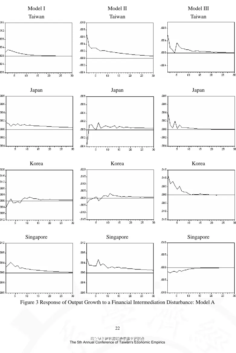
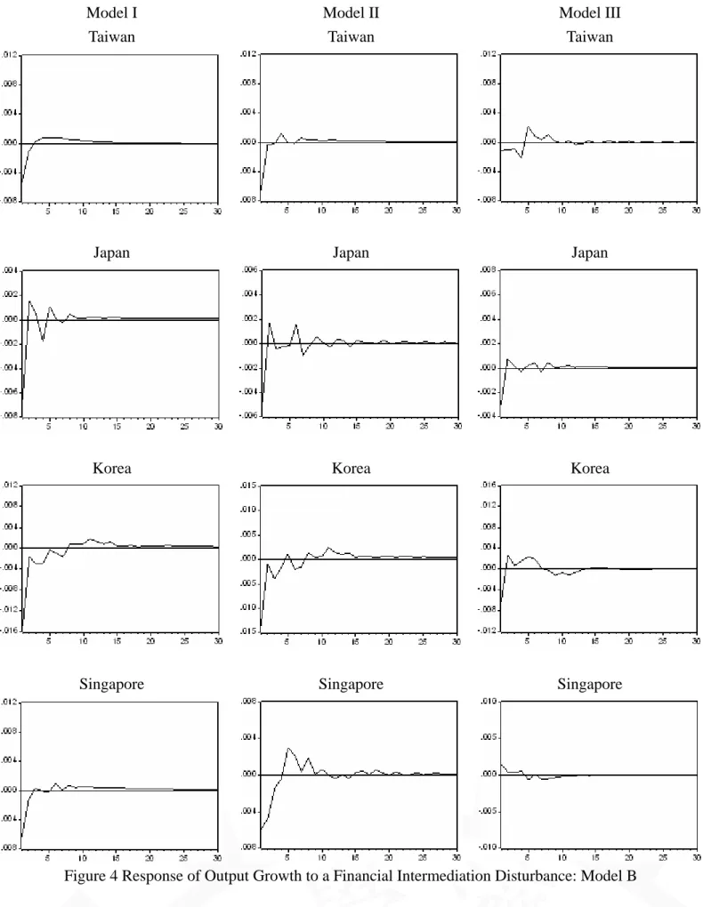
(20) 3.5 Sensitivity Analyses In this section, we investigate the sensitivity of our results into two alternative sets of long-run restrictions. In our small open economy system, let us reemphasize that, we view the world interest rate as the most exogenous variable in all plausible sets. In other words, true to the small open economy assumption, the world interest rate ordered first, followed by the other domestic variables. In addition, the ordering of government size, output, and money supply is natural and is consistent with theoretical models. Based on theoretical arguments, we suggest that there may be alternative orderings in the consideration between financial intermediation and the other two real variables (government size and real output). In the first alternative, we assume that the financial intermediation is exogenous in the long-run. It is possible that financial market development may have long-run implications on government size. For instance, a universal banking system may provide better risk management and thus require less government regulation, which lowers the demand for public sector. That is, financial intermediation variable is not affected by all other domestic disturbances but its own shocks. The ordering of this system is world interest rate, financial intermediation, government size, output, and the money supply; we name this specification model A. In the second alternative, we assume that the financial intermediation is affected by technological shocks in the long-run. There is some reason to believe that the long-run path of financial intermediation might be influenced by technological advances in communications and information processing. The ordering of the system is as follows: world interest rate, government size, output, financial intermediation, and money supply. We name this specification model B. By altering the ordering of the shocks, we generate a range of estimates on the importance of each of the shocks. By comparing the alternative results over various long-run specifications, we can draw some conclusions about the robustness of our results at the business cycle frequency. Using three different proxies for financial intermediation, both model A and B were estimated three times. The impulse response functions for output growth were described in Figure 3 and 4. Table 7 and 8 give the variance decomposition results. As displayed in Figure 5, the historical decomposition results of model A also yield quite identical patterns with the benchmark model. While the historical decomposition for model B can not be compared to the benchmark decompositions because the restrictions in model B are that the level of output does not respond to the financial intermediation shocks. The impulse response functions indicate that the estimated dynamic response of output to a one-standard-deviation financial intermediation shock is very robust to the alternative specifications. For each financial intermediation proxy, there is nearly no 20 第五屆全國實證經濟學論文研討會 The 5th Annual Conference of Taiwan's Economic Empirics.

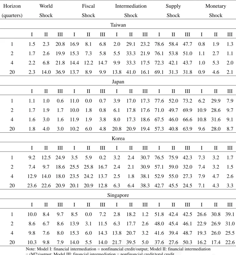
(21) difference in the estimated response among the benchmark model, model A and model B. The variance decomposition results indicate that they are virtually unchanged from the benchmark model. The only difference is that in model B for Japan financial intermediation is more important than in the benchmark case. For example, at the four-quarter horizon for Japan, the range for benchmark model is 6.2-14.3 (across the financial intermediation proxies) for the portion of output growth’s forecast error attributed to financial intermediation disturbances. The range was 8.0-18.6 for model A and larger range 9.6-54.7 for model B. For Korea, the benchmark model gave a range of 2.1 to 27.0. The range was 1.8-38.1 for model A and 6.9-36.6 for model B. For Singapore, the similar range in the benchmark model is 0.4-16.0, 3.2-20.7 for model A and 0.7-20.3 for model B. For Taiwan the range is 11.6-15.3 for benchmark model, 9.9-33.3 for model A and 3.4-20.2 for model B. Finally, the historical decompositions in Model A are nearly the same with the benchmark model. Both the patterns and magnitudes between benchmark model and model A are surprising good in Taiwan, Japan, Korea and Singapore. To sum up, the sensitivity results of impulse response functions and variance decomposition are very robust to the benchmark model. The historical decomposition of model A is also accord well with the benchmark decompositions. Thus, the evidence strong and significantly suggests that financial intermediation do generate the fluctuations of output growth.. 21 第五屆全國實證經濟學論文研討會 The 5th Annual Conference of Taiwan's Economic Empirics.

(22) Model I Taiwan. Model II Taiwan. Model III Taiwan. Japan. Japan. Japan. Korea. Korea. Korea. Singapore. Singapore. Singapore. Figure 3 Response of Output Growth to a Financial Intermediation Disturbance: Model A. 22 第五屆全國實證經濟學論文研討會 The 5th Annual Conference of Taiwan's Economic Empirics.

(23) Model I Taiwan. Model II Taiwan. Model III Taiwan. Japan. Japan. Japan. Korea. Korea. Korea. Singapore. Singapore. Singapore. Figure 4 Response of Output Growth to a Financial Intermediation Disturbance: Model B. 23 第五屆全國實證經濟學論文研討會 The 5th Annual Conference of Taiwan's Economic Empirics.

(24) Table 7 Variance Decomposition of Output Growth’s Forecast Error: Model A Horizon. World. Fiscal. Intermediation. Supply. Monetary. (quarters). Shock. Shock. Shock. Shock. Shock. Taiwan I. II. 1. 1.5. 2.3. 2. 1.7. 4 20. III. I. II. III. I. 20.8 16.9. 8.1. 6.8. 2.0. 2.6. 19.9 15.3. 7.3. 5.8. 2.2. 6.8. 21.8 14.4 12.2 14.7. 2.3. 14.0 36.9 13.7. 8.9. 9.9. II. III. I. II. III. I. II. III. 29.1 23.2 78.6 58.4 47.7. 0.8. 1.9. 1.3. 5.5. 33.3 21.9 76.1 53.8 51.0. 1.1. 2.7. 1.1. 9.9. 33.3 17.5 72.3 42.1 43.7. 1.0. 5.3. 2.0. 13.8 41.0 16.1 69.1 31.3 31.8. 0.9. 4.6. 2.1. I. II. III. 6.2. Japan I. II. III. I. II. III. I. II. III. I. II. III. 1. 1.1. 1.0. 0.6. 11.0. 0.0. 0.7. 3.9. 17.0 17.3 77.6 52.0 73.2. 29.9. 7.9. 2. 1.7. 1.9. 1.7. 10.0. 1.8. 0.8. 6.1. 17.8 17.6 71.0 49.7 69.9 10.9 28.6. 9.7. 4. 1.6. 3.0. 1.6. 11.9. 1.9. 3.8. 8.0. 17.3 18.6 67.5 46.0 66.6 10.8 31.6. 9.1. 20. 1.8. 4.0. 3.0. 10.2. 6.0. 4.8. 20.8 20.9 19.4 57.3 40.8 63.9. 9.6. 28.0. 8.7. I. II. III. Korea I. II. III. I. II. III. I. II. III. I. II. III. 3.5. 5.9. 0.2. 3.2. 2.4. 30.7 76.5 75.9 42.3. 7.3. 3.2. 1.7. 1. 9.2. 12.5 24.9. 2. 7.4. 9.7. 18.6 25.5 25.8 16.7. 2.4. 2.1. 30.9 57.1 59.0 32.0. 7.4. 3.2. 1.5. 4. 12.9 14.0 18.0 23.5 24.2 13.7. 2.5. 1.8. 38.1 52.9 55.0 27.3. 7.9. 4.7. 2.6. 20. 23.6 22.6 20.9 20.1 20.9 12.8. 6.3. 6.4. 38.3 42.7 45.5 24.5. 7.1. 4.3. 3.3. I. II. III. Singapore I. II. III. I. II. III. I. II. III. I. II. III. 1. 10.0. 8.4. 9.7. 8.5. 0.0. 7.2. 2.8. 18.2. 1.2. 51.8 42.4 42.5 26.6 30.8 39.1. 2. 8.6. 6.7. 8.6. 13.9. 3.1. 11.5. 6.3. 17.7. 2.6. 48.0 45.4 46.1 22.9 26.9 31.0. 4. 9.8. 7.6. 8.0. 15.3. 6.0. 14.3 13.8 20.7. 3.2. 41.6 39.4 48.7 19.3 26.0 25.5. 20. 10.3. 9.8. 7.9. 14.0. 5.5. 14.0 21.7 39.5. 5.0. 37.6 27.6 50.3 16.2 17.4 22.6. Note: Model I: financial intermediation = nonfinancial credit/output; Model II: financial intermediation = (M2)/output; Model III: financial intermediation = nonfinancial credit/total credit.. 24 第五屆全國實證經濟學論文研討會 The 5th Annual Conference of Taiwan's Economic Empirics.

(25) Table 8 Variance Decomposition of Output Growth’s Forecast Error: Model B Horizon. World. Fiscal. Intermediation. Supply. Monetary. (quarters). Shock. Shock. Shock. Shock. Shock. Taiwan I. II. III. I. II. III. I. II. III. 1. 1.5. 2.3. 20.8. 12.1 24.5 16.1 15.0 28.6. 0.8. 2. 1.7. 2.6. 19.9. 10.1 24.3 14.2 12.3 25.5. 4. 2.2. 6.8. 21.8. 9.0. 20. 2.3. 14.0. 36.9. 8.6. I. II. III. I. II. III. 70.4 42.5. 60.7. 0.8. 1.9. 1.3. 1.3. 74.6 44.6. 63.2. 1.1. 2.7. 1.1. 30.7 20.5 11.2 20.2. 3.4. 76.4 36.7. 51.9. 1.0. 5.3. 2.0. 27.0 14.6 11.5 14.6. 4.2. 76.4 39.5. 42.0. 0.9. 4.6. 2.1. II. III. I. II. III. Japan I. II. III. I. II. III. I. II. III. I. 1. 1.1. 1.0. 0.6. 8.5. 11.6. 6.7. 62.0 31.3 11.5 21.9. 26.0. 73.1. 6.2. 29.9. 7.9. 2. 1.7. 1.9. 1.7. 8.2. 11.1. 6.4. 58.3 33.4 11.6 20.7. 24.8. 70.3. 10.9. 28.6. 9.7. 4. 1.6. 3.0. 1.6. 11.0 11.7. 6.2. 54.7 28.9. 9.6. 21.5. 24.5. 73.2. 10.8. 31.6. 9.1. 20. 1.8. 4.0. 3.0. 10.4 13.0. 6.0. 47.2 25.0. 9.5. 30.8. 29.7. 72.5. 9.6. 28.0. 8.7. III. I. II. III. I. II. III. Korea I. II. III. I. II. III. I. II. 1. 9.2. 12.5. 24.9. 2.4. 5.6. 6.0. 54.4 43.6. 9.1. 26.4 34.9. 58.1. 7.3. 3.2. 1.7. 2. 7.4. 9.7. 18.6. 23.7 25.4 27.6 41.1 34.0. 8.1. 20.3 27.4. 43.9. 7.4. 3.2. 1.5. 4. 12.9 14.0. 18.0. 22.2 23.9 24.8 36.6 31.0. 6.9. 20.2 26.1. 47.4. 7.9. 4.7. 2.6. 20. 23.6 22.6. 20.9. 19.5 20.7 23.3 30.9 27.5. 7.4. 18.7 24.6. 44.9. 7.1. 4.3. 3.3. III. I. II. III. Singapore I. II. III. I. II. III. I. II. III. I. II. 1. 10.0. 8.4. 9.7. 7.7. 6.4. 8.4. 20.5 19.5. 1.0. 34.9 34.7. 41.6. 26.6. 30.8 39.1. 2. 8.6. 6.7. 8.6. 12.4 11.4 13.7 16.6 23.8. 0.8. 39.2 30.9. 45.6. 22.9. 26.9 31.0. 4. 9.8. 7.6. 8.0. 13.2 18.0 17.1 12.5 20.3. 0.7. 45.0 27.8. 48.4. 19.3. 26.0 25.5. 20. 10.3. 9.8. 7.9. 11.7 22.7 17.4 11.0 17.0. 0.9. 50.5 32.9. 51.0. 16.2. 17.4 22.6. Note: Model I: financial intermediation = nonfinancial credit/output; Model II: financial intermediation = (M2)/output; Model III: financial intermediation = nonfinancial credit/total credit.. 25 第五屆全國實證經濟學論文研討會 The 5th Annual Conference of Taiwan's Economic Empirics.

(26) Model I: Contribution of (CNF/RGDP) to Output. Figure 5 Historical Decomposition of Output Due to Financial Intermediation shocks: Model A 26 第五屆全國實證經濟學論文研討會 The 5th Annual Conference of Taiwan's Economic Empirics.

(27) 4. Conclusion This paper investigates the effect of financial intermediation on business cycles in Taiwan, Japan, Korea, and Singapore. We employ foreign, domestic variables, and three financial indicators to give an insight into this issue. Our empirical evidence suggests that the financial intermediation disturbances play an important role in generating business cycles in these small open economies. These financial intermediation shocks are separate from foreign interest rate, fiscal/monetary policy or output technology induced disturbances. We find that the dynamic responses of output to financial intermediation shocks display similar patterns in all cases across countries; however, the magnitude of the one-standard-deviation shock completely differs. These findings are also consistent with those from Lehr and Wang (2000) and Chang and Wang (2003). The only difference from Chang and Wang (2003), in particular, is that the magnitude of output response to financial intermediation shocks is relatively large in Taiwan and Singapore, while it is much smaller in Japan and Korea. Our results indicate that financial intermediation shocks were important in driving business cycles in small open economies, especially for Singapore and Taiwan.. 27 第五屆全國實證經濟學論文研討會 The 5th Annual Conference of Taiwan's Economic Empirics.

(28) References Beck, T., R. Levine, and N. Loayza (2000), “Finance and the Sources of Growth,” Journal of Financial Economics, 58, 261-300. Bencivenga V. R. and B. D. Smith, (1991), “Financial intermediation and endogenous growth,” Review of Economic Studies, 58(1), 195-209. Bencivenga V.R., B.D. Smith, and R.M. Starr (1995), "Transactions Costs, Technological Choice, and Endogenous Growth," Journal of Economic Theory, 67 (1), 153-177. Blanchard, O. J. and Quah, D. (1989) “The Dynamic Effects of Aggregate Demand and Supply Disturbances,” American Economic Review, 79, 655-673. Boyd, J., and E. Prescott, (1986), “Financial intermediary coalitions,” Journal of Economic Theory, 38, 211-232. Chang, S.H. and C.S. Mao (1997), “Post-War Taiwan’s business cycles: the small open economy and the international capital mobility” Taiwan Economic Review, 25:3. Chang, S.H. and P.W. Wang (2003), “The effects of financial intermediation on business cycle-Empirical study on four East Asia countries,” Taiwan Economic Annual Conference Paper. (In Chinese) Cooley, T. and S. Leroy (1985), “Atheoretical Macroeconomics：A Critique,” Journal. of Monetary Economics, 16, 283-308. Demetriades, P. O. and K. A. Hussein (1996), “Does Financial Development Cause Economic Growth? Time-Series Evidence from 16 Countries,” Journal of Development Economics, 51, 387-411. Demirgüç, K.A. and V. Maksimovic (1996), "Financial Constraints, Uses of Funds, and Firm Growth: An International Comarison," World Bank mimeo. Diamond, D. (1984), “Financial intermediation and delegated monitoring,” Review of Economic Studies, 51, 393-414. Enders, W. (1995), Applied Econometric Time Series, John Wiley & Sons, Inc. Engle, R.F. and C.W.J. Granger (1987), “Co-integration and Error Correction: Representation, Estimation, and Testing,” Econometrica, 55, 251–276. Galí, J., (1992), “How well does the IS-LM model fit postwar U.S. data?” Quarterly Journal of Economics, 107(2):709-738. Goldsmith, Raymond W., (1969), Financial structure and development, New Haven, CT: Yale University Press Granger, C. and P. Newbold (1974), "Spurious regressions in econometrics," Journal of Econometrics, 2, 111-20 Greenwood, J. and B. Jovanovic (1990), “Financial Development, Growth and 28 第五屆全國實證經濟學論文研討會 The 5th Annual Conference of Taiwan's Economic Empirics.

(29) Thedistribution of Income, ”Journal of Political Economy, 98(5), 1076- 88. Hoshi T. and H.T. Patrick (2000), Crisis and Change in the Japanese Financial System, Kluwer Academic Publishers, Boston Hardbound. Johansen, S. (1988) “Statistical Analysis of Cointegration Vectors,” Journal of Economic Dynamics and Control, 12, 231-254. Johansen, S. and K., Juselius (1990) “Maximum Likelihood Estimation and Inference on Cointegration – with Application to the Demand for Money,” Oxford Bulletin of Economics and Statistics, 52, 169-210. Johansen, S. (1991), “Estimation and Hypothesis Testing of Cointegration Vectors in Gaussian Vector Autoregressive Models,” Econometrica, 59, 1551–1580. Johansen, S. (1995), Likelihood-based Inference in Cointegrated Vector Autoregressive Models, Oxford University Press. King, R.G. and R. Levine（1993a）, “Finance and growth: Schumpeter might be right,”. Quarterly Journal of Economics, 108, 717-738. King, R.G. and R. Levine（1993b）, “Finance, entrepreneurship, and growth: theory and evidence,” Journal of Monetary Economics, 32, 513-542. Lehr, C.S. and P. Wang (2000), “Dynamic effects of financial intermediation over the business cycle,” Economic Inquiry, 38, 34-57. Levine, R. (1997), "Financial Development and Economic Growth: Views and Agenda," Journal of Economic Literature, 35, 688-726. Levine, R. and S. Zervos (1998), “Stock markets, banks, and economic growth,” American Economic Review, 88(3), 537-559. Levine, R., N. Loayza, and T. Beck (2000), “Financial Intermediation and Growth: Causality and Causes,” Journal of Monetary Economics, 46, 31-77. Lucas, R.E., Jr. (1988), “Money Demand in the United States: A Quantitative Review; A Comment,” Carnegie - Rochester Conference Series on Public Policy, 29. McKinnon, J. G. (1991), “Critical Values for Cointegration Tests,” Chapter 13 in R. F. Engle and C. W.J. Granger (eds.), Long-run Economic Relationships: Readings in Cointegration, Oxford University Press, 267-276. McKinnon, R.I. (1973), Money and capital in economic development, Washington, DC: The Brookings Institution. Odedokun, M.O. (1996), "Alternative Econometric Approaches for Analyzing the Role of the Financial Sector in Economic Growth: Time-Series Evidence from LDCs," Journal of Development Economics,.50, 119-46. Osterwald-Lenum, M. (1992), “A Note with Quantiles of the Asymptotic Distribution of the Maximum Likelihood Cointegration Rank Test Statistics,” Oxford Bulletin of Economics and Statistics, 54, 461–472. Patrick H.T. and Y.C. Park (1994), The Financial Development of Japan, Korea and 29 第五屆全國實證經濟學論文研討會 The 5th Annual Conference of Taiwan's Economic Empirics.

(30) Taiwan: Growth, Repressions and Liberalization, Oxford University Press. Schumpeter, J.A. (1911), The Theory of Economic Development, Harvard University Press, Cambridge, MA. Shaw, E.S. (1973), Financial Deepening in Economic Development, Oxford University Press, London and New York. Sims, C.A. (1980), "Macroeconomics and Reality," Econometrica, 48 (1), 1-48 The Bank of Korea (1990), Financial System in Korea, Seoul. World Bank (1999), Singapore: Selected Issues, IMF Staff Country Report No. 99/35.. 30 第五屆全國實證經濟學論文研討會 The 5th Annual Conference of Taiwan's Economic Empirics.

(31)