具資源感知能力之間接關聯串流探勘通用型架構

全文

(1)國立高雄大學資訊工程研究所碩士論文. 具資源感知能力之間接關聯串流探勘通用型架構 A Generic Framework for Resource-Aware Mining over Data Streams – Illustration of Indirect Associations Mining. 研究生: 楊順發指導教授:林文揚博士洪宗貝博士中華民國一百零一年一月. I.

(2) 致謝能夠完成這篇論文,首先要感謝我的指導教授林文揚老師以及洪宗貝老師, 林文揚老師儘管在我碩二時出國，仍不間斷的與我 meeting，進行研究相關的討論，在我對研究方面有問題時為我解惑，尤其在老師回國後，在我論文撰寫的這段期間，時常要讓老師修改到半夜,學生除了感到慚愧外，也萬分感激老師為學生這樣無私的付出。洪宗貝老師對於我在研究方面思考不周全的地方，點出需要注意的重點，以及該如何去尋求解決的方法。洪老師也時常提醒學生在報告論文方面要怎麼加強,如何舉例子才能讓人很快的聽懂，學生真是受益匪淺，十分感謝您的教導。兩位老師除了研究相關事情外，也經常的關心學生的生活近況，學生覺得能夠當老師的學生真是太好了，再次感謝兩位老師這樣無微不至的照顧。同時我也要感謝我的口試委員曾新穆教授、曾守正教授，感謝你們撥冗參加我的口試,並提出寶貴的建議，使我的論文能夠更加完善。在來要感謝實驗室博士班的國誠學長、浚瑋學長以及明泰學長，在我對 paper 有問題時，經常的麻煩你們了。碩士班的長隆學長、佑恩學長、憶清學長和電機系的奇峰，不論是修課方面或是生活遇到的大小事都可以找你們討論。宗慶及學弟嘉蔚、弘裕與新程,在我準備口試忙不過來的時候，助我一臂之力，幫忙分擔口試的準備工作。謝謝你們大家。最後我要感謝我的父母，一直以來體諒我這不成熟的兒子，默默的為我付出，使我無後顧之憂，因為有你們我才有繼續下去的動力。. II.

(3) 具資源感知能力之間接關聯串流探勘通用型架構指導教授: 林文揚博士國立高雄大學資訊工程研究所. 共同指導教授:洪宗貝博士國立高雄大學資訊工程研究所. 學生: 楊順發國立高雄大學資訊工程研究所. 中文摘要在知識爆炸、新興技術蓬勃發展的時代裡，資訊產生的速度幾乎快到讓我們無法分析，也不太可能將所有收集到的資料儲存在有限的儲存裝置中，使得目前針對靜態資料為主的探勘技術無法適用在這種新的資料型態。在本篇論文中，我們的目標是開發出一個具有資源感知能力的通用探勘架構來探勘間接的關聯規則，使其能夠根據資料產生的速度以及目前可用的系統資源，例如處理器的效能及記憶體的可用空間，來調整計算的速度及記憶空間的消耗量。我們提出一個基於 GIAMS 架構，具有資源感知能力的通用型間接關聯規則的探勘架構，稱之為 RA-GIAMS。. III.

(4) 此架構可以掌握系統資源如處理器及記憶體空間的變化，在不增加太多的額外計算以及維持產生出的規則的正確性的考量下，儘可能地運用目前可用的資源來完成間接關聯規則探勘的工作。針對記憶體感知能力的設計，我們提出了一個可動態調節用以儲存潛在頻繁項目集的資料結構的大小的演算法，此演算法可在記憶體不足時尋找適當的節點加以修剪。經由在人造與實際資料集的實驗驗證，我們的方法可以有效地調節記憶體的消耗，而對所找出的間接關聯規則的正確性不致於造成太大的影響。關鍵字: 資源感測、串流探勘、間接關聯、自我調節架構、頻繁項目集。. IV.

(5) A Generic Framework for Resource-Aware Mining over Data Streams – Illustration of Indirect Associations Mining. Advisor: Dr. Wen-Yang Lin Institute of Computer Science and Information Engineering National University of Kaohsiung. Co-Advisor: Dr. Tzung-Pei Hong Institute of Computer Science and Information Engineering National University of Kaohsiung. Student: Shun-Fa Yang Institute of Computer Science and Information Engineering National University of Kaohsiung. Abstract As the advent of emerging techniques in the information explosion age, data accumulates faster than it can be analyzed, and it is nearly impossible to store a stream entirely in a persistent storage, which makes contemporary mining algorithms designed for static dataset awkward and inapplicable to cope with such new types of dataset.. V.

(6) In this thesis, we aim at developing a generic framework to mining indirect association rules with resource-aware capability that can adapt the computation in accordance with data arriving rate as well as the available resources, including CPU power and memory space. We propose a generic framework RA-GIAMS, an extension the GIAMS framework with resource-awareness capability that can cope with the variation of available resources, including both CPU power and memory space, and make use of most available resources to accomplish the discovery of indirect association rules without too much overhead and retaining as could as possible the accuracy of discovered rules. To realize the memory awareness scheme, we propose a victim searching and node releasing algorithm to adjust the structure for maintaining potential frequent itemsets in accordance with the available memory space. Empirical evaluations on both synthetic and real datasets show our algorithm can efficiently adjust the size of the structure without sacrificing too much the accuracy of discovered indirect association rules. Keywords: Resource-awareness, stream mining, indirect association, adaptation scheme, frequent itemset.. VI.

(7) Content 致謝............................................................................................................................II 中文摘要.................................................................................................................III Abstract ....................................................................................................................V List of Figures .......................................................................................................IX List of Table ...........................................................................................................XI CHAPTER 1 Introduction.................................................................................1 1.1 Motivation......................................................................................................1 1.2 Contributions..................................................................................................3 1.3 Thesis Organization........................................................................................4. CHAPTER 2 Background and Related Work............................................5 2.1 Indirect Association Mining...........................................................................5 2.2 Resource-Aware Stream Mining....................................................................8. CHAPTER 3 GIAMS: A Review...................................................................11 3.1 The Generic Framework...............................................................................11 3.2 The Generic Algorithm.................................................................................14. CHAPTER 4 The Proposed Resource-Aware GIAMS Framework..16 4.1 Framework Overview...................................................................................16 4.2 Notation Description....................................................................................18 4.3 Adaption Scheme for CPU Power Awareness..............................................19 4.3.1 Basic Concept............................................................................................19 4.3.2 CPU Efficiency and Workload Estimation................................................21 4.3.3 An Example...............................................................................................22 4.4 Adaption Scheme for Available Memory Awareness...................................23 4.4.1 Basic Concept...........................................................................................24 4.4.2 Algorithm Description...............................................................................28 4.4.3 An Example...............................................................................................31. VII.

(8) CHAPTER 5 Experimental Results.............................................................38 5.1 Experiment Design.......................................................................................38 5.2 Evaluation on Real Dataset..........................................................................38 5.3 Evaluation on Synthetic Dataset...................................................................45. CHAPTER 6 Conclusions and Future Work............................................50 6.1 Conclusions..................................................................................................50 6.2 Future Work..................................................................................................51. References..............................................................................................................52. VIII.

(9) List of Figures Figure 2-1 Indirect association mining algorithm..........................................................6 Figure 3-1 The generic window model used in GIAMS..............................................12 Figure 3-2 The GIAMS generic framework for indirect association mining...............13 Figure 3-3 The GIAMS algorithm................................................................................15 Figure 4-1 The proposed RA-GIAMS framework.......................................................17 Figure 4-2 CPU awareness scheme..............................................................................20 Figure 4-3 An example data stream..............................................................................22 Figure 4-4 An illustration of Card-Stree* ...................................................................24 Figure 4-5 An illustration of victim-list.......................................................................26 Figure 4-6 Algorithm description of DelayInsert.........................................................29 Figure 4-7 Algorithm for victim searching & releasing...............................................30 Figure 4-8 The itemsets maintained in an example Card-Stree*.................................31 Figure 4-9 The Card-Stree* and victim-list after inserting ABCD..............................32 Figure 4-10 The Card-Stree* and victim-list after inserting ABC...............................33 Figure 4-11 The Card-Stree* and victim-list after inserting ABD...............................34 Figure 4-12 The Card-Stree* and victim-list after inserting ABE...............................35 Figure 4-13 The Card-Stree* and victim-list after inserting ACD...............................36 Figure 4-14 The Card-Stree* and victim-list after deleting ABCD and ABD.............37 Figure 5-1 Execution times of RA-GIAMS running over msnbc with available memory variation....................................................................................40 Figure 5-2 Execution times spent on node replacement running over msnbc with available memory variation.......................................................................40 Figure 5-3 Error rate of discovered frequent itemset from msnbc with available memory variation.......................................................................................41 Figure 5-4 Average support error of discovered frequent itemsets from msnbc with available memory variation.......................................................................42 Figure 5-5 Precisions of RA-GIAMS in terms of discovered indirect associations from msnbc with available memory variation....................................................44 Figure 5-6 Recalls of RA-GIAMS in terms of discovered indirect associations from msnbc with available memory variation.................................................45 Figure 5-7 Execution times of RA-GIAMS running over T5I5N0.1KD1000K with available memory variation.......................................................................46 Figure 5-8 Execution times spent on node replacement running over T5I5N0.1KD1000K with available memory variation..............................47 Figure 5-9 Error rate of discovered frequent itemsets from T5I5N0.1KD1000K with available memory variation.......................................................................47. IX.

(10) Figure 5-10 Average support error of discovered frequent itemsets from T5I5N0.1KD1000K with available memory variation...........................48 Figure 5-11 Precisions of RA-GIAMS running on T5I5N0.1KD1000K with available memory variation....................................................................................49 Figure 5-12 Recalls of RA-GIAMS running on T5I5N0.1KD1000K with available memory variation....................................................................................49. X.

(11) List of Table Table 2-1 A summary of related work on resource-aware stream mining....................10 Table 4-1 Notation used in the design of RA-GIAMS.................................................18 Table 5-1 Parameter settings for generic window model used in this experiment.......39 Table 5-2 Characteristics of the test data msnbc..........................................................39 Table 5-3 Characteristics of the test data T5I5N0.1KD1000K....................................45. XI.

(12) CHAPTER 1 Introduction 1.1 Motivation. As the advent of emerging techniques in the information explosion age, e.g., internet, handheld devices, RFID, sensor network, e-commerce, etc., more and more systems or applications would generate continuous rapid flow of vast data in a timely and endless fashion. This heralds a new type of data source, called data streams, and brings new challenges to the data mining research community. Unlike traditional static data sources, streaming data is fast changing, continuously generated and unbounded in amount. That is, data usually accumulates faster than it can be analyzed, and it is nearly impossible to store a stream entirely in a persistent storage, which makes contemporary mining algorithms designed for static dataset awkward and inapplicable to cope with such new type of dataset. Recent studies on stream data mining have achieved some general requirements for effective mining algorithms [9], including single-pass of scanning over data set, real-time execution, and low memory consumption. Not until recently, however, researchers have begun to pay attention to another critical and more challenging issue, adaptive mining of streaming data with respect to variations in available resources, i.e., CPU power and memory space. For example, almost all types of mobile devices are embedded with constrained resources, including memory, battery, and CPU computing capability.. 1.

(13) Any mining algorithm running on these resources constrained devices has to be able to adjust and adapt its execution to utilize the very limited, changing in availability resources. Contemporary research work on resource-aware mining over data streams can be viewed from two aspects, the type of resources under concern, e.g., CPU power [8] or memory space [10], and the type of mining tasks employed, e.g., clustering [18], density estimation [16], frequent itemset mining [8, 21], etc. Most studies conducted from the viewpoint of resource type consider either CPU power or memory space, but not both; the issue that how to take both types of resources simultaneously into account to develop efficient and adaptive mining algorithms remains unexplored. From the viewpoint of data mining task, almost all works were focusing on frequent pattern discovering; no work, to our knowledge, has been devoted to the problem of mining infrequent patterns, e.g., indirect associations. Another minor restriction of the previous works is that they were conducted with respect to some specific stream window model, e.g., landmark, time-fading, or sliding window. Algorithms tailored for some particular window model usually are not applicable to and so need redesigning to fit to other models. In this thesis, we aim at developing a generic mining framework with resource-aware capability that can adapt the computation in accordance with data arriving rate as well as the available resources, including CPU power and memory space. As a first step toward the realization of the generic framework, we focus on the mining of indirect associations [19], a type of infrequent patterns that reveal infrequent itempairs yet highly co-occurring with a frequent itemset called “mediator”.. 2.

(14) We propose a generic framework RA-GIAMS with resource-awareness capability, which is an extension the GIAMS framework [14, 25] that can represent all classical streaming models and retain user flexibility in defining new models. Our RA-GIAMS framework can cope with the variation of available resources, including both CPU power and memory space, and make use of most available resources to accomplish the discovery of indirect association rules without too much overhead and retaining as could as possible the accuracy of discovered rules. To realize the memory awareness scheme, we propose a victim searching and node releasing algorithm to adjust the structure for maintaining potential frequent itemsets in accordance with the available memory space. Empirical evaluations on both synthetic and real datasets show our algorithm can efficiently adjust the size of the structure without sacrificing too much the accuracy of discovered indirect association rules.. 1.2 Contributions The main contributions of this thesis are summarized as follows: 1.. We propose a generic stream data mining framework with resource-aware. capability which can adapt the computation in accordance with data arriving rate as well as the available resources, including CPU power and memory space. 2.. We illustrate how the proposed framework can be applied to the discovery. of indirect association rules. Specifically, we design two kernel functionalities, the adaptation schemes for CPU computing power variability and available memory space variability, respectively. To the best of our knowledge, this is the first study for resource-aware mining of indirect associations over data streams.. 3.

(15) 3.. We propose an efficient victim searching and node releasing algorithm to. realize the adaptation scheme for available memory. Experimental results show this algorithm can effectively adjust the memory consumption during the course of frequent pattern mining without sacrificing too much of the accuracy of discovered rules.. 1.3 Thesis Organization The remainder of this thesis is organized as follows. In Chapter 2, we provide some background knowledge and related work about indirect association mining, data stream window model, resource-aware stream mining, and load shedding. Since our work in this study is based on the GIAMS framework, a generic stream window model and algorithmic framework for indirect association rules mining, we give an overview of GIAMS and the algorithm in Chapter 3. Chapter 4 describes our proposed GIAMS-RW framework, an extension of GIAMS with resource-aware capability, including the revised system framework, the algorithmic design for adaptive functionalities with respect to CPU-power and memory space variation, respectively, and the detailed data structure and procedure for realizing the algorithmic framework. Chapter 5 then describes the series of experiments we conducted on evaluating the proposed framework. We considered both synthetic and real datasets and examined the effects of various factors, e.g., data arrival rate, CPU-power, available memory space. Finally, the conclusions and future work of this thesis are presented in Chapter 6.. 4.

(16) CHAPTER 2 Background and Related Work 2.1 Indirect Association Mining The concept of mining indirection association was first proposed by [19] for discovering the useful infrequent patterns beyond the association rules. To facilitate the presentation of our framework, we first give a formal definition of indirect associations below. Definition 1 An indirect association rule is denoted as. x, y M , meaning that. an itempair {x, y} is indirectly associated by a mediator set M if the following conditions hold: 1. sup({a, b}) < σ s (Itempair support condition); 2. sup({a} ∪ M) ≥ σ f and sup({b} ∪ M) ≥ σ f. (Mediator support condition);. 3. dep({a}, M) ≥ σ d and dep({b}, M) ≥ σ d (Mediator dependence condition); where sup(A) denotes the support of a itemset A, and dep(P, Q) is a measure of the dependence between itemsets P and Q. The factors σ s , σ f and σ d are described as follows. The first one σ s means that if the support of itemset is lower than this threshold then it is recognized as an infrequent itemset. The second σ f is the mediator support threshold that if the support of itemset is higher than it, then the itemset is a frequent itemset. Note that σ f ≥ σ s . The last one σ d denotes the dependence support threshold. Many functions can be used for measuring the dependence of itemsets. In this thesis, we follow the suggestion in [19, 20], adopting the well-known dependence function, IS measure.. 5.

(17) sup ( P, Q). IS ( P, Q) =. sup ( P) sup (Q) Existing researches on indirect association mining can be divided into two categories, either focusing on proposing more efficient mining algorithms or extending the definition of indirect association for different applications. The original indirect association mining approach proposed by [20] called “Indirect association mining algorithm” is shown in Figure 2-1. In general the algorithm could be divided into two phases, including frequent itemsets extract phase (step 1) and indirect associations mining (steps 2~7). However, it is time-consuming to generate all frequent itemsets before mining indirect association.. Algorithm: Indirect association mining algorithm Input: Transaction Database D, σ s , σ f , and σ d . Output: Indirect Associations IA. 1:. Extract frequent itemsets, Let L 1 , L 2 , …, L n be the set of frequent i-itemsets generated by any frequent base algorithm;. 2: 3: 4: 5: 6:. IA = ∅;. 7:. for k = 2 to n do C k+1 = join(L k , L k ); foreach {x, y}∪M ∈ C k+1 do if sup({x, y}) < σ s , dep({x}, M) ≥ σ d , dep({y}, M) ≥ σ d then IA = IA∪ {⟨x, y| M⟩}; endfor Figure 2-1. Indirect association mining algorithm. Wan and An [23] proposed an approach, called HI-mine, for improving the efficiency of the INDIRECT algorithm.. 6.

(18) Rather than generating all frequent itemsets, HI-mine focuses on finding all itempairs first, and then pursues the mediator of each itempair. The HI-mine algorithm adopts a data structure based on the concept of dynamic transaction projection of frequent item, through which there is no need for doing any join operation for candidate generation. Instead, Hi-mine generates two new sets, indirect itempair set and mediator support set, by recursively building the HI-struct for the database. Then indirect associations are discovered from these two sets directly. Later, Wan and An proposed an enhancement of the HI-mine algorithm, called HI-mine* [22]. HI-mine* adopts a more compact data structure call Super Compact Transaction Database (STDB), on which some optimization strategies are introduced, including only one database scanning, direct frequent item projecting, and dynamic infrequent item pruning. Chen et al. [6] also proposed an indirect association mining approach that was similar to HI-mine, namely MG-Growth. The differences between them are that the directed graph and bitmap are used in MG-Growth for constructing the indirect itempair set (IIS). The corresponding mediator graphs are then generated for deriving indirect associations. As to extending the definition of indirect association, Kazienko et al. [13] applied indirect association on web pages recommendation system. Chen et al. [6] proposed an approach for mining indirect association of items by adding time feature of goods. Since each item has its lifespan, the relationships of new coming items can thus easily be discovered.. 7.

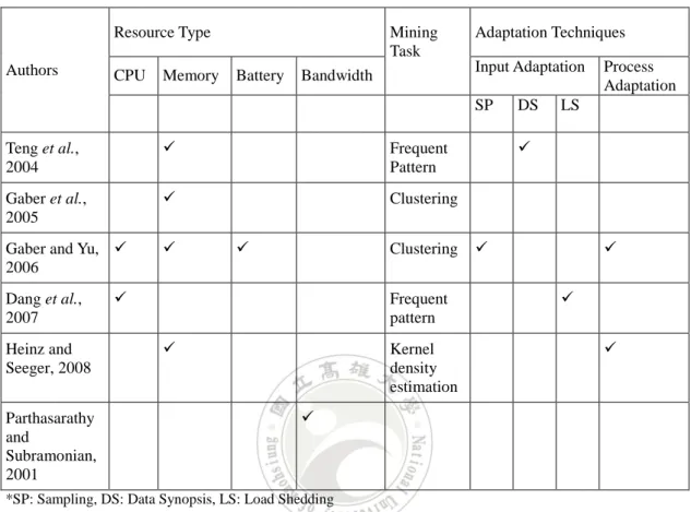
(19) 2.2 Resource-Aware Stream Mining The research of resource-aware stream mining focuses mainly on how to use the limited resources to efficiently accomplish the mining task while guarantee as could as possible the accuracy of mining results. Contemporary research work on resource-aware mining over data streams can be viewed from three aspects, the type of resources under concern, the type of mining tasks employed, and the type of adaption techniques used. Studies conducted from the viewpoint of resource type include in general situation, CPU power and memory space, or additional issues for mobile devices, battery and network bandwidth. The types of mining tasks studied include clustering, frequent pattern mining, kernel density estimation. Finally, the adaptation techniques can be input adaptation or algorithm adaptation. The input adaptation technique refers to schemes used in adjusting the amount of input data to keep up with the pace of the stream and meet the computing capacity. Three commonly used approaches including sampling, i.e., statistically choosing some input data, load shedding, i.e., discarding part of the input data, and data synopsis creation, referring to data summarization techniques that retain the data characteristics, statistics or profile. Teng et al. [21] proposed a wavelet based data synopsis technique, called RAM-DS (Resource-Aware Mining for Data Streams), to transform the input data stream into different granularity of data from temporal view or frequency view in order to reduce the data amount. Their work focused on frequent pattern mining. The group led by M.M. Gaber is one of the pioneers in resource-aware stream data mining.. 8.

(20) They have conducted a series of research studies on resource-awarestream clustering [10, 11], with ultimate goal at developing a general resource-aware framework that can adapt to variability of different resource availability over time. Their recent work [11] proposed a generic framework called Algorithm Granularity Settings, which uses three levels of adaptation strategies in the data input, algorithm processing, and data output, and cope with different issues of resource-awareness. The work conducted by Dang et al. [7, 8] considers stream mining under CPU resource constraint, focusing on frequent pattern discovery, and using load shedding technique. Their approach relies on a way to estimate the system workload by approximately computing the number of maximal itemsets that can be generated from a transaction, and then employs the load shedding technique to sample transactions if the system workload is over the current CPU computing power. Heinz and Seeger [16] proposed an algorithm adaptation method that is tailored to the problem of kernel density estimation. The resource type considered in their work is memory space. In distributed computing environment, the network bandwidth available for data transmission is particularly important. Parthasarathy and Subramonian [17] developed a resource-aware scheduling scheme to cope with the bandwidth limitation.. 9.

(21) A summary of the above work on resource-aware stream data mining is shown in Table 2-1. Table 2-1 A summary of related work on resource-aware stream mining. Resource Type Authors. CPU. Memory. Mining Task Battery. Adaptation Techniques Input Adaptation. Bandwidth. SP Teng et al., 2004. . Frequent Pattern. Gaber et al., 2005. . Clustering. Gaber and Yu,  2006. . Dang et al., 2007 Heinz and Seeger, 2008 Parthasarathy and Subramonian, 2001. . Clustering. . Frequent pattern . Kernel density estimation . *SP: Sampling, DS: Data Synopsis, LS: Load Shedding. 10. DS. Process Adaptation. LS. . .   .

(22) CHAPTER 3 GIAMS: A Review GIAMS (Generic Indirect Association Mining over Streams) [14, 25] is an algorithmic framework that can accommodates the three stream window model called Landmark model, Time-fading model and Sliding window, while retains user flexibility for defining new models. Users only have to set four variables (timestamp, window size, stride and decay rate) in accordance with the generic window model, then GIAMS can discover indirect association rules. Since our work in this thesis is based on this framework, in this chapter we give a brief review of this framework.. 3.1 The Generic Framework. Suppose that we have a data stream S = (t 0 , t 1 , t 2,... t i ,...), where t i denotes the transaction arrived at time i. Since data stream is a continuous and unlimited incoming data along with time, a window W usually is specified, representing the sequence of data arrived from t i to t j , denoted as W[i, j]=(t i , t i+1 , ..., t j ). GIAMS adopts a generic window model Ψ for data stream mining, which is dictated as a four-tuple specification, Ψ(l, w, s, d), where l denotes the timestamp at which the window start, w as the window size, s is the stride the window moves forward, and d is the decay rate. The stride notation s is introduced to allow the window moving forward in a batch of transactions (of size s).. 11.

(23) That is, if the current window under concern is (t j−w+1 , t j−w+2 , …, t j ), then the next window will be (t j−w+s+1 , t j−w+s+2 , …, t j+s ), and the weight of a transaction within (t j−s+1 , t j−s+2 , …, t j ), say α, is decayed to αd, and the weight of a transaction within (t j+1 , …, t j+s ) is 1. The concept of the proposed generic window model is depicted in Figure 3-1.. … … t0 t1. …. …. …. …. tl tj−ω+1tj−ω+2 tj−ω+s+1 tj−s+1 tjj tj+1. tj+s. time. Wk Wk+1. α αd. 1. Figure 3-1. The generic window model used in GIAMS [14].. The GIAMS framework is developed according to the paradigm proposed by Tan et al. [20]: First, discovers the set of frequent itemsets with support higher than σ f , and then generates the set of qualified indirect associations from the frequent itemsets. Based on this paradigm, GIAMS works in the following scenario: (1) The user first sets the streaming window model by specifying the parameters described previously; (2) The framework then executes the process for discovering and maintaining the set of potential frequent itemsets PF as the data continuously stream in;. 12.

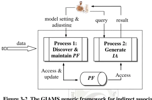
(24) (3) At any moment once the user issues a query about the current indirect associations the second process for generating the qualified indirect associations is executed to generate from PF the set of indirect associations IA. Figure 3-2 depicts the generic streaming framework for indirect associations mining.. model setting & adjusting. data. query. Process 1: Discover & maintain PF Access & update. result. Process 2: Generate IA. PF. Access. Figure 3-2. The GIAMS generic framework for indirect association mining [14].. 13.

(25) 3.2 The Generic Algorithm Based on the generic framework in Figure 3-3, the generic algorithm employed by GIAMS consists of two concurrent processes running simultaneously: PF-monitoring and IA-generation. The first process is activated when the users specifies the window parameters to set the type of window model, responsible for generating itemsets from the incoming block of transactions and inserting those that are potentially frequent into a repository called monitoring lattice. The second process is activated when the user issues a query about the current indirect associations, responsible for generating the qualified patterns from the frequent itemsets maintained by process PF-monitoring. A sketch of the generic algorithm is described in Figure 3-4.. 14.

(26) Algorithm Name: GIAMS Input: Itempair support threshold σ s , association support threshold σ f , dependence threshold σ d , decay rate d, window size w, support error threshold ε. Output: Indirect Associations IA. Initialization: 1. Let N be the accumulated number of transactions, N = 0; 2. Let η be the decayed accumulated number of transactions, η = 0; Let cbid be the current block id, cbid = 0, sbid the starting block id of 3. window, sbid = 1; 4. repeat 5. Process 1; 6. Process 2; 7. until terminate; Process 1: FP-monitoring 1. Reading the new coming block B i ; 2. cbid = cbid + 1; 3. N = N + s; η = η × d + s; 4. if ( N > ω) then 5. BlockDelete(sbid, FP); // Delete outdated block B sbid 6. sbid = sbid + 1; N = N – s; // Decrease the transaction size in current 7. window cbid – sbid+1 η = η – s×d ; // Decrease the decayed transaction size in 8. current window 9. endif 10. TransactionMerge(B cbid , CT); // Merge anological transactions into a compact table CT 11. DelayInsert(CT, FP, σ f , cbid, η); // Constructing FP using transactions in CT 12. Decay&Pruning(d, s, ε, cbid, FP); // Removing infrequent itemsets from FP Process 2: IA-generation 1. if user query request = true then IndirectAssociationGen(FP, σ f , σ d , σ s, N); // Generate all indirect 2. associations Figure 3-3. The GIAMS algorithm.. 15.

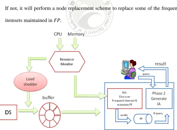
(27) CHAPTER 4 The Proposed Resource-Aware GIAMS Framework In this chapter, we describe our proposed resource-aware GIAMS framework, namely RA-GIAMS. We will first give an overview of RA-GIAMS, then focus on the design of two kernel functionalities, the adaptation schemes for CPU computing power variability and available memory space variability, respectively. 4.1 Framework Overview Based on the GIAMS framework proposed in [14, 25], our proposed RA-GIAMS add some mechanisms to cope with the variation of available resources, considering both CPU power and memory space, making use of most available resources to accomplish the discovery of indirect association rules. As depicted in Figure 4.1, the new components added into our RA-GIAMS include the resource monitor, responsible for monitoring the current CPU computing power and available memory space; the load shedder, responsible for throwing off part of the incoming data; a buffer, using as a temporary container for keeping the incoming data; and the storage shedder, responsible for pruning maintained frequent itemsets to reduce memory requirement. These new mechanisms work in the following scenario to realize the functionality of resource-awareness.. 16.

(28) 1. The resource monitor will periodically monitor the current CPU computing power and the available memory space. As we will show in later sections, the CPU computing power can be represented as the number of dominating operations accomplished within a time unit, and the memory usage can be represented as the amount of card-tree nodes, because each tree node consumes similar memory space. The information collected is then forwarded to the load shedder and storage shedder to take necessary action. 2. When the load shedder receives the CPU power information, it will compare this with the ongoing workload to see if it will exceed the estimated CPU computing power; if so, it will shed part of the input data. 3. Likewise, as the storage shedder receives the memory usage information, it will inspect if the available memory enough for processing the incoming transactions. If not, it will perform a node replacement scheme to replace some of the frequent itemsets maintained in FP.. Figure 4-1. The Proposed RA-GIAMS framework.. 17.

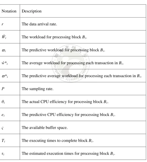
(29) 4.2 Notation Description Before we proceed to the detailed design of adaptation schemes, we describe in this section the notation that will be used. The description is presented in Table 4-1.. Table 4-1 Notation used in the design of RA-GIAMS. Notation. Description. r. The data arrival rate.. Ŵi. The workload for processing block B i .. ϖi. The predictive workload for processing block B i .. ŵ* i. The average workload for processing each transaction in B i .. ϖ* i. The predictive average workload for processing each transaction in B i .. Ρ. The sampling rate.. θi. The actual CPU efficiency for processing block B i .. ei. The predictive CPU efficiency for processing block B i .. ς. The available buffer space.. Ti. The executing times to complete block B i .. τi. The estimated execution times for processing block B i .. 18.

(30) 4.3 Adaption Scheme for CPU Power Awareness. In this section, we will present the design of the adaption scheme for CPU power awareness.. 4.3.1 Basic Concept. The basic concept of our design is depicted in Figure 4.2., where the buffer is regarded as a circular queue. Conforming to the generic window model used in GIAMS, we assume that the input stream is processed block by block. After the completion of the (i-1)th block B i−1 , the resource monitor can calculate the CPU current efficiency θ i-1 and predict the CPU efficiency e i for processing the i-th block B i . A simple estimation taking the actual efficiency and predictive efficiency into account described in Eq. (4.1) is used, where α denotes a weight, 0 ≤ α ≤ 1; if α is higher than 0.5 means that the estimated efficiency is more important than the actual one. Although we would use other more complicated estimation methods, in this study we prefer simpler methods to avoid too much computation overhead.. e i = α θ i-1 + (1 − α) e i−1. 19. (4.1).

(31) Let ϖ I denote the estimated workload for processing block B i and ς is the available buffer space currently. Our intention is to ensure that during the course for processing block B i , the amount of arriving data will not over the available buffer size. If not, we then activate the load shedder to shed the input data with a sampling rate P. It is not hard to derive the value of P to satisfy this situation.. P × r × τi ≤ ς. (4.2). P ≤ ς / (r × τ i ). (4.3). That is,. where the estimated execution times for processing B i will be τ i = ϖ i / e i .. Figure 4-2. CPU awareness scheme.. 20.

(32) 4.3.2 CPU Efficiency and Workload Estimation. In the description of the basic concept for our adaptation scheme for CPU awareness, there are two key points need further clarification. They are the CPU efficiency monitoring and the estimation of the workload ϖ I for processing block B i . The CPU efficiency, though the meaning is intuitively simple, i.e., the number of operations can be accomplished within a time unit, is not easy to monitor and calculate in real time. Our idea is to cope with the estimation from a computation complexity viewpoint. First, we observe that the most time-consumption procedure of algorithm GIAMS (see Figure 3-3) is the delay insert, which is responsible for decomposing transactions into itemsets and maintaining frequent patterns. The most important operations of delay insert are the node creation, update, and replacement (will illustrate at the memory awareness). For this reason, we can represent the CPU efficiency as the amount of these operations accomplished within one second. The actual CPU efficiency θ i for completing the process of block B i can be defined as θi = ŵi / ti. (4.4). where ŵ i denotes the number of operations, including node insertion, update and replacement, for completing B i and t i is the execution time. The workload estimation ϖ i for processing B i , however, needs employing a different strategy because this has to be done before block B i is processed.. 21.

(33) Our idea is estimating the average number of operations needed to process a transaction by using the statistics collected in processing the previous block B i−1 . Let ŵ* i−1 and ϖ* i-1 be the actual and estimated average number of operations to process a transaction for block B i−1 , respectively. That is, ŵ* i−1 = ŵ i−1 / |B i−1 | and ϖ* i−1 =. ϖ i−1 / |B i−1 |. Then we can estimate ϖ* i in the same way for estimating CPU efficiency.. ϖ* i = α ŵ* i−1 + (1 − α)ϖ* i−1. (4.5). And so, we have ϖ i = ϖ* i × |B i |.. 4.3.3 An Example Consider the example stream in Figure 4-3. There are three blocks of transactions, the block B 3 is just finished and the block B 4 is going to be processed, and block B 5 is store in the buffer; the block 6 is new generated from stream. We assume that the predictive CPU efficiency of e 3 is equal to 21; the workload of ŵ 3 is equal to 36 and takes 2 seconds; the predictive workload ϖ 3 is equal to 42; the available buffer space ς = 2; the data arrival rate r = 3; and the estimation weight α = 0.5. Block6. Block5. Tid 12 AE Tid 13 ACE. Block4. Tid 9 ACE Tid 10 AD Tid 11 BCD. Block3. Tid 6 ABC Tid 7 ACD Tid 8 BCD. Figure 4-3. An example data stream.. 22.

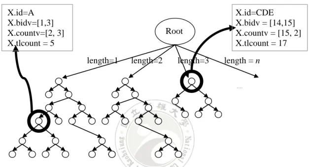
(34) We first calculate the CPU efficiency θ 3 = 36/2 = 19 and predict the CPU efficiency during the course for processing block B 4 , e 4 = 0.5*19 + 0.5*21 = 20. The average transactional workload for processing block B 3 , ŵ* 3 = 36/3 = 12; and predictive counterpart ϖ* 3 = 42/3 = 14. Then we can predict the average transactional workload for processing block B 4 , calculated as ϖ* 4 = 0.5*12 + 0.5*14 = 13. So we have ϖ 4 = 13*(3) = 39 and the estimated execution time will be τ 4 = 39/20 = 1.95. Finally we obtain the sample rate P = 2 / (3 ×1.95) = 2/8.4 = 34.18%.. 4.4 Adaption Scheme for Available Memory Awareness In this section, we describe the adaption scheme for available memory awareness. Recall that our framework relies on the maintenance of promising frequent itemsets, PF. Our concern thus is how to deal with the situation that available memory is not enough to hold all the frequent itemsets maintained in PF, and develop an adaptive scheme for adjusting PF to utilize the most of current available memory space. The structure used in our RA-GIAMS for realizing PF is a modification of the tree structure used in GIAMS, called Card-Stree, which is a forest of search trees keeping itemsets of different cardinalities, appearing in the current window, say ST 1 , ST 2 , …, ST k , for ST k maintaining the set of frequent k-itemsets. We name the modified structure Card-Stree*. Each node in Card-Stree* except the root keep the information of the maintained itemset. More specifically, for each itemset X, the node records X.id, the identifier of X; X.bidv, the vector of identifiers of the blocks that X appears;. 23.

(35) X.countv, the vector that stores the number of occurrences of X within each block; and X.tlcount, the total number of times that X appears in the current window under concern. An example of Card-Stree* is depicted in Figure 4-4. Because each node consumes approximately the same amount of memory space, in what follows we use a node as the memory unit.. X.id=A X.bidv=[1,3] X.countv=[2, 3] X.tlcount = 5. X.id=CDE X.bidv = [14,15] X.countv = [15, 2] X.tlcount = 17. Root length=1. length=2. length=3. length = n ...... Figure 4-4. An illustration of Card-Stree*.. 4.4.1 Basic Concept A simple and intuitive approach is blindly dropping some itemsets while the memory space is not enough. However, it is very likely too much information will loss, making the mining results incorrect and leading to wrong analysis. Rather, we employ a strategy similar to the concept of cache replacement. That it, when the memory space is insufficient, we decide which itemsets in the current Card-Stree* are less important and can be deleted to release enough space for accommodating the incoming, more important itemsets.. 24.

(36) In this regard, we propose a node releasing mechanism to cope with the situation when memory space is not enough to maintain all of potential frequent itemsets in the Card-tree*. Note that the processing of stream mining needs to be computed in real time. As such, the main design concern of our approach is the efficiency, i.e., how to efficiently search and determine the victim nodes for deletion, without sacrificing too much the accuracy of the discovered rules. First, we note that for mining indirect association, the set of 2-itemsets is the most important set, because from which all length-2 mediators and the infrequent itempairs are generated. As such, our node replacement is executed only when the memory space is not enough and the new generated itemsets from the incoming transaction are of lengths 1 and 2. In other words, those new generated k-itemsets with k > 2 are discarded immediately when the memory is not enough. Second, considering that the frequency of long itemsets is usually less than that of short itemsets, and the lengthy rules constructed from long itemsets are less understandable to the users, our approach replaces nodes according to their cardinalities, first choosing the longest itemsets. More precisely, suppose that we need to release n nodes, and k denotes the largest length of itemsets in Card-Stree*. Our approach will search for the top n nodes with the smallest counts in the ST k subtree. If there are less than n nodes found in ST k , then the search continues in subtrees ST k-1 , ST k-2 , and so on. However, during the search process, we will delete any node whose count is equal to 1 and decrement the number of nodes to be released. This is because these nodes represent the least occurring itemsets.. 25.

(37) Third, to facilitate the search of n victim nodes, we introduce a link structure called victim-list to maintain the nodes in Card-Stree* chosen for deletion. Each node in victim-list contains three fields, the count of the itemsets, the number of itemsets having this count, and pointers to all the corresponding nodes in the Card-Stree*. All nodes in victim-list are sorted in decreasing order of counts. Figure 4-5 illustrates the structure of victim-list. Below we summarize the main steps for searching and eliminating victim nodes using the victim-list structure. 1. If there exist new generated 1- or 2-itemsets need to be inserted but the memory space is not enough, figure out the amount of nodes n need to be deleted, and call the node releasing procedure in step 2.. Figure 4-5. An illustration of victim-list. 2. For each subtree in Card-Stree*, starting from ST k , inspect each node X and execute the following substeps to determine if choosing X as a victim and inserting it into victim-list.. 26.

(38) 2-1. If X.tlcount = 1, delete X and decrease n by 1. Then check the number of victims stored in the first node victim-list[0]. If the total number of victims maintained in victim-list, say #victim, subtract victim-list[0].num is at least n, then eliminate victim-list[0] and update #victim. 2-2. Else if the number of nodes in victim-list is less than n, then insert X into victim-list in decreasing order of count. 2-3: Else, perform either one of the following cases. case 1: The count of X is larger than that of the first node in victim-list. Skip X and continue to inspect the next node in ST k . case 2: The count of X is equal to that of the first node in victim-list. Insert X into the first node and update victim-list[0].num and victim-list[0].pointer. case 3: The count of X is less than that of the first node in victim-list. In this case, we first insert X into victim-list. Then check the number of victims stored in the first node victim-list[0]. If the total number of victims maintained in victim-list, say #victim, subtract victim-list[0].num is at least n, then eliminate victim-list[0] and update #victim. 3. If the number of victims in victim-list is less than n and k – 1 < 2, then k = k – 1 and go to step 2 (searching the next subtree ST k-1 ). 4. Eliminate all victims maintained in victim-list from Card-Stree* and insert at most #victim new generated itemsets into Card-Stree*. There are some remarks noticeable in the aforementioned procedure before we proceed to the detailed algorithm description. First, the victims are maintained and deleted in groups, distinguishing by count. That is why we may end up with more than n victims in victim-list. Second, for efficiency concern, we only compare the count of the inspecting node X with that of the first group in victim-list (see step 3).. 27.

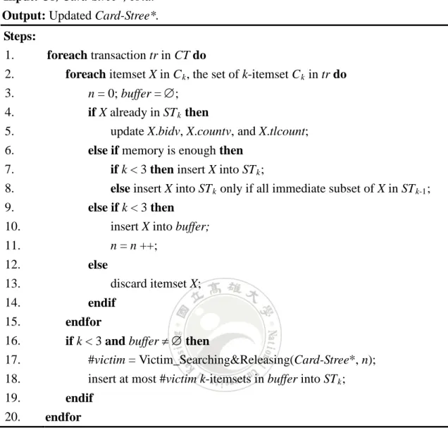
(39) This avoids the overhead for linear searching along the entire victim-list.. 4.4.2 Algorithm Description We first present the algorithm description of DelayInsert, which is responsible for constructing and maintaining Card-Stree* using transactions in CT, then detail the victim searching & releasing algorithm, which acts as a procedure called by DelayInsert when the memory shortage does occur. The algorithm DelayInsert is described in Figure 4-6. In summary, for each k-itemset X generated from the input transaction, if X is already in Card-Stree*, update its information. Otherwise, if the memory space is enough, then insert X if k < 3, or perform delay insert if k ≥ 3. On the other hand, if the memory is not enough and k ≥ 3, then we simply discard itemset X. But for k < 3, we temporarily store X into a buffer. After all itemsets in C k have been inspected, then call algorithm Victim_Searching&Releasing to release memory, and insert at most #victim of the new generated k-itemsets in buffer into Card-Stree*.. 28.

(40) Procedure Name: DelayInsert Input: CT, Card-Stree*, cbid. Output: Updated Card-Stree*. Steps: 1. foreach transaction tr in CT do 2. foreach itemset X in C k , the set of k-itemset C k in tr do 3. n = 0; buffer = ∅; 4. if X already in ST k then 5. update X.bidv, X.countv, and X.tlcount; 6. else if memory is enough then 7. if k < 3 then insert X into ST k ; 8. else insert X into ST k only if all immediate subset of X in ST k-1 ; 9. else if k < 3 then 10. insert X into buffer; 11. n = n ++; 12. else 13. discard itemset X; 14. endif 15. endfor 16. if k < 3 and buffer ≠ ∅ then 17. #victim = Victim_Searching&Releasing(Card-Stree*, n); 18. insert at most #victim k-itemsets in buffer into ST k ; 19. 20.. endif endfor Figure 4-6. Algorithm description of DelayInsert. 29.

(41) Algorithm: Victim searching & releasing Input: Number of nodes n and Card-Stree* Output: Number of victim nodes releasing from Card-Stree*, #victim 1: 2 3: 4: 5: 6: 7: 8: 9: 10: 11: 12: 13: 14: 15: 16: 17: 18: 19: 20: 21: 22: 23: 24: 25:. #victim = 0; k = the largest length of itemsets in Card-Stree*;. 26: 27: 28: 29: 30:. k = k − 1; until #victim >= n or k = 2; foreach victim X in victim-list do delete the corresponding nodes pointed by X.addr from Card-Stree*;. repeat for each node X in subtree of length k, ST k do if X.tlcount = 1 then delete node X from Card-Stree*; n = n − 1; if #victim − victim-list[0].num >= n then delete victim-list[0]; endif if #victim < n then insert node X into victim-list; #victim++; else if #victim >= n then compare X.tlcount with victim-list[0].count; case 1: > ; case 2: = insert node X into victim-list;. #victim++;. case 3: insert node X into victim-list; #victim++; if #victim − victim-list[0].num >= n then delete victim-list[0]; #victim = #victim – victim-list[0].num; endif endif endfor. return #victim; Figure 4-7. Algorithm for victim searching&releasing The algorithm for finding victim for releasing is described in Figure 4-7, which. details the steps implementing the idea presented in subsection 4.4.1.. 30.

(42) 4.4.3 An Example Suppose the Card-Stree* contains the set of frequent itemsets shown in Figure 4-8. For simplicity, we only show the total counts of each itemsets. Suppose that we want to insert F and G into Card-Stree* but found the memory is not enough. Then the procedure Victim_Searching&Releasing is activated to perform victim searching and node releasing, with n = 2.. Figure 4-8. The itemsets maintained in an example Card-Stree*.. 31.

(43) 1. The victim search starts from itemsets in subtree of length 4, i.e., ST 4 . Since the victim-list is empty, itemset ABCD is inserted into victim-list with count = 3 and link to its corresponding node in Card-Stree*. The result is shown in Figure 4-9.. Figure 4-9. The Card-Stree* and victim-list after inserting ABCD.. 32.

(44) 2. Since there are other subtrees with cardinality larger than 2 and #victim < n, the victim search continues to subtree of cardinality 3, first inspecting the node ABC. Since #victim < 2 and ABC’s count is larger than 3, so we insert ABC to the front of victim-list. The result is shown in Figure 4-10.. Figure 4-10. The Card-Stree* and victim-list after inserting ABC.. 33.

(45) 3. The search process continues to examine other nodes in subtree ST 3 . The next node inspected is ABD. Note that its count is 4, smaller than that of ABC, and so we insert ABD into victim-list. However, we found #victim – victim-list[0].num = 2. Therefore, ABC is deleted. The result is shown in Figure 4-11.. Figure 4-11. The Card-Stree* and victim-list after inserting ABD.. 34.

(46) 4. The next node is ABE. Its count is 2, smaller than that of ABD. So ABE is inserted into victim-list. Again, since #victim – victim-list[0].num = 2, node ABD is deleted. The result is shown in Figure 4-12.. Figure 4-12. The Card-Stree* and victim-list after inserting ABE.. 35.

(47) 5. The next node is ACD. Its count is 3 equal to the first node ABCD in victim-list. So, we insert ACD to the same node wherein ABCD locates, as shown in Figure 4.13.. Figure 4-13. The Card-Stree* and victim-list after inserting ACD.. 36.

(48) 6. The next itemset is ACE. Its count is equal to 1, so we delete immediately the node containing ACE from ST 3 and decrease the number of nodes for releasing by 1, obtaining n = 1. After this, we found there are far more victims in victim-list than required, i.e., #victim – victim-list[0].num ≥ n, so delete the first group in victim-list. The result is depicted in Figure 4-14.. Figure 4-14. The Card-Stree* and victim-list after deleting ABCD and ABD.. 7. The next node is BCD. Since its count is larger than that of the first node in victim-list, i.e., 2, we ignore BCD. 8. Finally, all nodes in ST 3 have been inspected and #victim = 1, equal to required. Hence, we delete from Card-Stree* all of the nodes pointed by the victims in victim-list to release memory for inserting F and G.. 37.

(49) CHAPTER 5 Experimental Results 5.1 Experiment Design To evaluate the effectiveness and efficiency of RA-GIAMS, we conducted a series of experiments on both synthetic and real datasets. The evaluation was inspected from two aspects, execution time and pattern accuracy. All experiments were done on Intel(R) Core(TM) i5-2400(3.1G) PC with 4GB of main memory, running the Windows 7 32-bit operation system. All programs were implemented in Visual C++ 2008.. 5.2 Evaluation on Real Dataset In this experiment, we consider the sliding window model, with detail settings of the generic model shown in Table 5-1. The dataset msnbc [2] is used, which was constructed from the web log of news pages in msn.com for the entire day of September, 28, 1999. The characteristics of msnbc are summarized in Table 5-2. More detailed description of this dataset can be found in [2].. 38.

(50) Table 5-1. Parameter settings for generic window model used in this experiment. s. w. d. σs. σf. σd. 10000. 80000. 1. 0.01. 0.01. 0.1. Table 5-2. Characteristics of the test data msnbc. Database. Items. Transactions. Maximum Transaction size. Average Transaction size. msnbc. 17. 989818. 17. 1.71678. To inspect the performance and effectiveness of our memory awareness adaptation scheme, we run RA-GIAMS under five settings of available memory, i.e., ranging from 90% to 50% of the original memory space, with 10% decrement. And compare the results with those running with sufficient memory space. First, we evaluate the execution times of RA-GIAMS. The results are depicted in Figure 5-1. As the results demonstrate, most of the time RA-GIAMS is faster than GIAMS even RA-GIAMS incurs overhead for running victim searching and node releasing to cope with insufficient memory. And the execution times increase as the available memory increase. This is because when the memory is not sufficient there are certain amount of itemsets that originally have to be maintained in the Card-Stree* are pruned, which has the effect in decreasing the number of create and update operations, without doing too much of node replacement operations, as shown in Figure 5-2, where the cases of 70%, 80% and 90% memory incur the least number of node replacement operations.. 39.

(51) Figure 5-1. Execution times of RA-GIAMS running over msnbc with available memory variation.. Figure 5-2. Execution times spent on node replacement running over msnbc with available memory variation.. 40.

(52) Next, we inspect the accuracy of the results generated by RA-GIAMS. Because our algorithm introduces storage shedder to prune itemsets to be maintained in the Card-Stree* structure, so error may occur to the discovered frequent itemsets, including the missing rate and support error of frequent itemsets, and the precision and recall with respect to indirect association rules. We first evaluate how much of frequent itemsets generated by GIAMS without memory limitation will be lost when memory shortage occurs, which is measured as error rate: Error = |F true ∩ F est | / |F true |. (5.1). where F true denotes the set of frequent itemsets discovered by GIAMS while F est represents that by RA-GIAMS with insufficient memory.. Figure 5-3. Error rate of discovered frequent itemsets from msnbc with available memory variation.. 41.

(53) We then check the difference between the supports of the discovered frequent itemsets with and without memory limitation, which is measured by the following formula called ASE (Average Support Error):. ASE =. ∑ (Tsup( x) − Esup( x)) x∈F. F. (5.2). where Tsup denotes the frequent itemsets that are discovered by GIAMS, Esup denotes the frequent itemsets discovered by RA-GIAMS under memory limitation. As the results displayed in Figure 5-4, all ASEs are nearly zero in all cases, even in the case that only 50% of memory is available.. Figure 5-4. Average support error of discovered frequent itemsets from msnbc with available memory variation.. 42.

(54) We then examine the accuracy of rules discovered by RA-GIAMS. We consider two measurements, precision and recall. Let IA true denote the set of indirect associations discovered by GIAMS without memory limitation and IA est denote the set discovered by RA-GIAMS with insufficient memory. The precision measures the ratio of how many indirect associations in IA est are also in IA true , while recall examines the percentage of how many indirect associations in IA true are missed generated by RA-GIAMS. These two criteria are define as follows:. Precision = |IA true ∩ IA est | / |IA est |. (5.3). Recall = |IA true ∩ IA est | / |IA true |. (5.4). As the results illustrated in Figures 5-5 and 5-6, the memory adaptation scheme of our RA-GIAMS performs very well. All of the precisions are larger than 0.9 and recalls are above 0.8, meaning the percentages of false indirect associations discovered by our RA-GIAMS are less than 10% and the percentages of true indirect associations not discovered by RA-GIAMS are less than 20%, respectively, even in the case that only 50% of memory is available.. 43.

(55) Figure 5-5. Precisions of RA-GIAMS in terms of discovered indirect associations from msnbc with available memory variation.. 44.

(56) Figure 5-6. Recalls of RA-GIAMS in terms of discovered indirect associations from msnbc with available memory variation.. 5.3 Evaluation on Synthetic Dataset In this experiment, we consider a synthetic dataset T5I5N0.1KD1000K generated by the IBM data generator, whose characteristics are summarized in Table 5-3. The parameter settings for generic window model follow the settings for msnbc.. Table 5-3. Characteristics of the test data T5I5N0.1KD1000K. Database. Items. T5I5N0.1KD1000K 17. Transactions 767768. Maximum Transaction size 23. Average Transaction size 6.23. We first examine the performance of RA-GIAMS over this dataset. As the results depicted in Figure 5-7, surprisingly, we can see the execution times of 90% and 80% memory are more than the execution time without memory limitation.. 45.

(57) The reason is that both cases incur much more node replacement operations than the other cases, as shown in Figure 5-8.. Figure 5-7. Execution times of RA-GIAMS running over T5I5N0.1KD1000K with available memory variation.. We next inspect the errors of the generated frequent itemsets. As the results shown in Figures 5-9 and 5-10, all of the errors are nearly zero in all cases.. 46.

(58) Figure 5-8. Execution times spent on node replacement running over T5I5N0.1KD1000K with available memory variation.. Figure 5-9. Error rate of discovered frequent itemsets from T5I5N0.1KD1000K with available memory variation.. 47.

(59) Finally, we inspect the precision and recall in terms of indirect association rules. As the results illustrated in Figures 5-11 and 5-12, all cases exhibit very high precision and recall, nearly one.. Figure 5-10. Average support error of discovered frequent itemsets from T5I5N0.1KD1000K with available memory variation.. 48.

(60) Figure 5-11. Precisions of RA-GIAMS running on T5I5N0.1KD1000K with available memory variation.. Figure 5-12. Recalls of RA-GIAMS running on T5I5N0.1KD1000K with available memory variation.. 49.

(61) CHAPTER 6 Conclusions and Future Work 6.1 Conclusions In this thesis, we have considered the problem of resource-aware mining of indirect association rules over data streams. We have proposed a generic framework RA-GIAMS to cope with this problem. Our proposed framework is based on GIAMS, a mining framework that can accommodate most of the contemporary stream window models and allow user-defined specific window models. Our framework add some mechanisms to GIAMS, including a resource monitor, a load shedder, and a storage shedder, as a whole can adapt the computation in accordance with data arriving rate as well as the available resources, including CPU power and memory space. To evaluate the effectiveness and performance of the proposed framework, we have conducted a series of experiments. The experimental results showed that our framework can effectively adjust the memory consumption during the course of frequent pattern mining with very little overhead. In addition, the results also showed that even with limited memory space, i.e., only 50% of the original space, our framework not only can discover most of the frequent patterns serving as mediators for qualified indirect associations but also maintain the accuracy of discovered patterns; the support errors are very small, nearly zero in all test settings.. 50.

(62) 6.2 Future Work In this thesis, we only complete the implementation of the proposed adaption schemes for available memory awareness. In the future, we will accomplish the scheme for or CPU power awareness and integrate it to the RA-GIAMS. The study of resource-aware mining from streaming data is still in its infancy. Many research issues are worthy of further investigation. Among many topics to be explored in the future, some important ones are listed below: 1.. In this study, we confine the resources to the general types, CPU power and. memory space. Many applications developed in mobile environment, such as sensor networks, intelligent cell phones, however, have to consider additional resources constraint, mainly battery and network bandwidth. We will extend our framework to accommodate these new types of resources. 2.. It is interesting to note that although our proposed framework RA-GIAMS. aims at discovering indirect association rules, it relies on a kernel procedure for generating frequent itemsets, whose discovery is the most computation-intensive part to many mining tasks, such as association rules, classification, and clustering. In this regard, we believe that our framework can be extended to accomplish these tasks, developed as a more general data stream mining system.. 51.

(63) References [1]. B. Babcock, M. Datar, and R. Motwani, “Load Shedding Techniques for Data Stream Systems,” in Proceedings of the 2003 Workshop on Management and Processing of Data Streams, 2003.. [2]. I. Cadez, D. Heckerman, C. Meek, P. Smyth, and S. White, “Visualization of Navigation Patterns on a Web Site Using Model-Based Clustering,” in Proceedings of the 6th ACM SIGKDD International Conference on Knowledge Discovery and Data Mining, pp. 280-284, 2000.. [3]. J. H. Chang, H. C. Kum, “Frequency-Based Load Shedding over A Data Stream of Tuples,” Information Sciences, vol. 179, no. 21, pp. 3733-3744, 2009.. [4]. J. H. Chang, and W. S. Lee, “estWin: Adaptively Monitoring the Recent Change of Frequent Itemsets over Online Data Streams,” in Proceedings of 12th International Conference on Information and Knowledge Management, pp. 536-539, 2003.. [5]. J. H. Chang, and W. S. Lee, “Find Recent Frequent Itemsets Adaptively over Online Data Stream,” in Proceedings of 9th ACM SIGKDD International Conference on Knowledge Discovery and Data Mining, pp. 487-492, 2003.. [6]. L. Chen, S. S. Bhowmick, and J. Li, “Mining Temporal Indirect Associations,” in Proceedings of 10th Pacific-Asia Conference on Knowledge Discovery and Data Mining, pp. 425-434, 2006.. [7]. X. H. Dang, W. K. Ng, and K. L. Ong, “Adaptive Load Shedding for Mining Frequent Patterns from Data Streams,” in Proceedings of Data Warehousing and Knowledge Discovery, pp. 342-351, 2006.. 52.

(64) [8]. X. H. Dang, W. K. Ng, K. L. Ong, and V. C. S. Lee, “Discovering Frequent Sets from Data Streams with CPU Constraint,” in Proceedings of 6th Australasian Data Mining Conference, pp. 121-128, 2007.. [9]. P. Domingos and G. Hulten, “A General Framework for Mining Massive Data Streams,” Journal of Computational and Graphical Statistics, vol. 12, no. 4, pp. 945-949, 2003.. [10] M. M. Gaber, S. Krishnaswamy, and A. Zaslavsky, “Resource-aware Mining of Data Streams,” Journal of Universal Computer Science, vol. 11, no. 8, pp. 1440-1453, 2005. [11] M. M. Gaber and P. S. Yu, “A Framework for Resource-aware Knowledge Discovery in Data Streams: A Holistic Approach with Its Application to Clustering,” in Proceedings of ACM Symposium on Applied Computing, pp. 649-656, 2006. [12] P. Kazienko, “IDRAM—Mining of Indirect Association Rules,” in Proceedings of International Conference on Intelligent Information Processing and Web Mining, pp. 77-86, 2005. [13] P. Kazienko and K. Kuzminska, “The Iinfluence of Indirect Association Rules on Recommendation Ranking Lists,” in Proceedings of 5th International Conference on Intelligent Systems Design and Applications, pp. 482-487, 2005. [14] W. Y. Lin, Y. E. Wei, and C. H. Chen, “A Generic Approach for Mining Indirect Association Rules in Data Streams,” in Proceedings of 24th International Conference on Industrial, Engineering and Other Applications of Applied Intelligent Systems, pp. 95-104, 2011.. 53.

(65) [15] S. Guha, A. Meyerson, N. Mishra, and R. Motwani, “Clustering Data Streams: Theory and Practice,” IEEE Transactions on Knowledge and Data Engineering, vol. 15, no. 3, pp. 515-258, 2003. [16] C. Heinz, and B. Seeger, “Cluster Kernels: Resource-Aware Kernel Density Estimators over Streaming Data,” IEEE Transactions on Knowledge and Data Engineering, vol. 20, no. 7, pp. 880-893, 2008. [17] S. Parthasarathy, and R. Subramonian, “An Interactive Resource-Aware Framework for Distributed Data Mining,” IEEE Technical Committee on Distributed Processing Letters, pp. 24-32, 2001. [18] R. Shah, S. Krishnaswamy, and M. M. Gaber, “Resource-Aware Very Fast K-Means for Ubiquitous Data Stream Mining,” in Proceedings of 2nd International Workshop on Knowledge Discovery in Data Streams, pp. 40-50, 2005. [19] P. N. Tan, V. Kumar, and J. Srivastava, “Indirect Association: Mining Higher Order Dependencies in Data,” in Proceedings of 4th European Conference on Principles of Data Mining and Knowledge Discovery, pp. 632-637, 2000. [20]. P. N. Tan and V. Kumar, “Mining Indirect Associations in Web Data,” in Proceedings of 3rd International Workshop on Mining Weg Log Data Across All Customers Touch Points, pp. 145-166, 2001.. [21] W. G. Teng, M. S. Chen and P. S. Yu, “Resource-Aware Mining with Variable Granularities in Data Streams,” in Proceedings of SIAM Conference on Data Mining, pp. 22-24, 2004 [22] J. X. Yu, Z. Chong, H. Lu, Z. Zhang, and A. Zhou, “A False Negative Approach to Mining Frequent Itemsets from High Speed Transactional Data Streams,” Information Sciences, vol. 176, no. 14, pp. 1986-2015, 2006.. 54.

(66) [23] Q. Wan, and A. An, “An Efficient Approach to Mining Indirect Associations,” Journal of Intelligent Information Systems, vol. 27, no. 2, pp. 135-158, 2006. [24] Q. Wan and A. An, "Efficient Indirect Association Discovery using Compact Transaction Databases," in Proceedings of 2006 IEEE International Conference on Granular Computing, pp. 154-159, 2006. [25] Y. E. Wei, A Generic Framework and Algorithms for Mining Indirect Associations from Data Streams, Master Thesis, National University of Kaohsiung, Taiwan, 2010.. 55.

(67)