利用計分檢定統計量之指數加權移動平均控制圖來監控一般線性輪廓

國

立

交

通

大

學

統計學研究所

碩

碩

碩

碩 士

士

士

士 論

論

論

論 文

文

文

文

利用計分檢定統計量之指數加權移動平均控制圖來監

控一般線性輪廓

An Exponentially Weighted Moving Average Control

Chart Based on Score Test Statistics for Monitoring

General Linear Profiles

研 究 生：馮千育

利用計分檢定統計量之指數加權移動平均控制圖來監控一般線

性輪廓

An Exponentially Weighted Moving Average Control Chart

Based on Score Test Statistics for Monitoring General Linear

Profiles

研 究 生：馮千育 Student：Chien-Yu Feng

指導教授：陳志榮 博士 Advisor：Dr. Chih-Rung Chen

國 立 交 通 大 學 理 學 院

統 計 學 研 究 所

碩 士 論 文

A Thesis

Submitted to Institute of Statistics

College of Science National Chiao Tung University in partial Fulfillment of the Requirements

for the Degree of Master

in Statistics April 2013

利用計分檢定統計量之指數加權移動平均控制圖來監

控一般線性輪廓

研究生：馮千育

指導教授：陳志榮 博士

國立交通大學統計學研究所碩士班

摘

要

摘

摘

要

要

摘

要

統計製程控制是常常用在監控工業實務的一個方法，其中控制圖更

是一個用重要的監控工具。本文提出利用計分檢定統計量的指數加權

移動平均來監控一般線性輪廓的資料。並且用模擬的方法來跟一些文

獻的資料做比較，來探討它的表現與優劣。

An Exponentially Weighted Moving Average Control Chart

Based on Score Test Statistics for Monitoring General Linear

Profiles

Student：Chien-Yu Feng

Advisor：Dr. Chih-Rung Chen

Institute of Statistics

National Chiao Tung University

Abstract

Statistical process control is often utilized to monitor an industrial process.

Control charts are important monitoring tools used to determine whether a process is

in a state of statistical control. An exponentially weighted moving average control

chart based on score test statistics to monitor general linear profiles is proposed in this

paper. The performance of the proposed monitoring scheme is compared with

references through a simulation study.

誌

謝

誌

謝

誌

謝

誌

謝

我的研究所生涯，比別人多的快一年的時間，一切都是自己平時

不認真的後果，現在終於能夠畢業了，實在非常感動。

首先我非常感謝我的指導教授-陳志榮老師，從二年級開始一直到

我畢業，比其他同學多了快一年的時間，老師依然未間斷的辛苦教導，

無論怎樣的問題老師都會詳細的跟我解說，並教導我嚴謹的研究態

度，老師對我的照顧，無限感激。此外也感謝替我口試的口試委員們，

感謝蔡明田教授特別遠從臺北下來新竹一趟，感謝許文郁教授感冒還

能特別前來，感謝洪志真教授給我論文的建議。

最後要感謝交大統計所的所有老師與工作人員們，讓我茫然無助

時能夠指引我學習研究的方向。特別還要感謝我的家人們，如不是你

們一直以來的包容及支持，我也不可能有今天的成就。

馮千育 謹誌于

國立交通大學統計學研究所

中華民國一百零二年四月

Contents

1 Introduction 1

1.1 Motivation . . . 1

1.2 Literature Review . . . 2

2 An EWMA control chart for monitoring general linear profiles 7 2.1 Model . . . 7

2.2 Known in-control process parameters without constraint . . . 8

2.3 Known in-control process parameters with constraint . . . 11

2.4 Unknown in-control process parameters without constraint . . . 13

2.5 Unknown in-control process parameters with constraint . . . 17

2.6 Proposed monitoring scheme . . . 18

3 A Simulation Study 21

4.3 Modify monitoring scheme (2) . . . 26

5 Future Work 29

References 30

List of Tables

5.1 Out of control ARL comparisons between EWMA with known in-control parameters and constraint case, ZTW, KMW and HEWMA charts for shifts in β0, where θj = (β0+ δ0σ, β1, σ)T and τj2 = 4δ02 for j ≥ 1. . . . . 32

5.2 Out of control ARL comparisons between EWMA with known in-control parameters and constraint case, ZTW, KMW and HEWMA charts for shifts in β1, where θj = (β0, β1+ δ1σ, σ)T and τj2 = 120δ21 for j ≥ 1. . . 32

5.3 Out of control ARL comparisons between EWMA with known in-control parameters and constraint case , ZTW, KMW and HEWMA charts for shifts in σ, where θj = (β0, β1, δσ)T for j ≥ 1. . . . 33

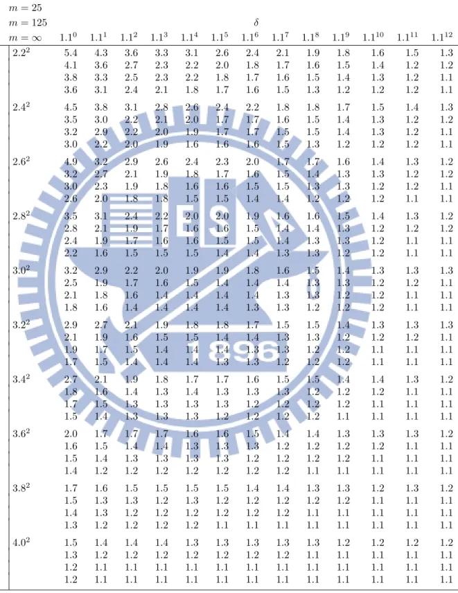
5.4 ARLs with unknown in-control parameters and constraint case for shifts in θ with θj = (βTj, δσ)T and τj2 = τ2/δ2 for j ≥ 1 . . . . 34

5.5 ARLs with unknown in-control parameters case for shifts in θ with θj =

(βT_j, δσ)T _{and τ}2

j = τ2/δ2 for j ≥ 1 . . . . 35

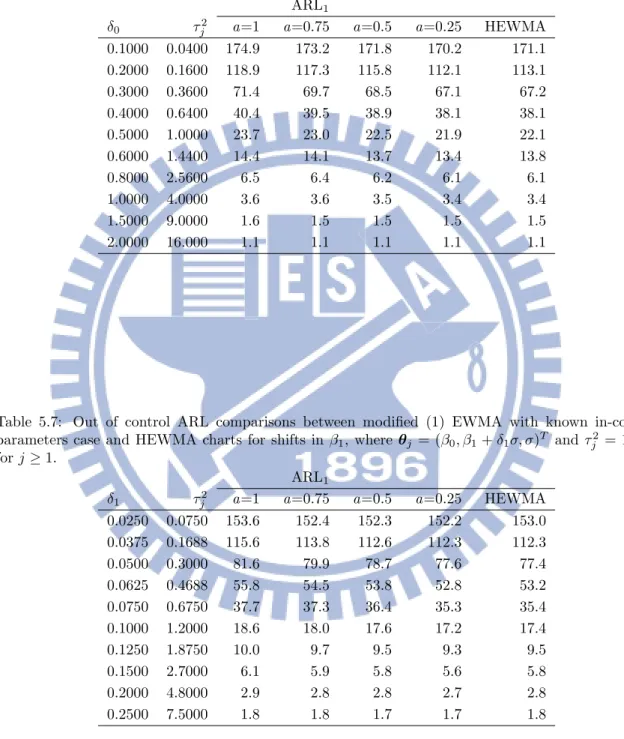
5.7 Out of control ARL comparisons between modified (1) EWMA with known in-control parameters case and HEWMA charts for shifts in β1,

where θj = (β0, β1+ δ1σ, σ)T and τj2 = 120δ12 for j ≥ 1. . . . 36

5.8 Out of control ARL comparisons between modified (1) EWMA with known in-control parameters case and HEWMA charts for shifts in σ, where θj = (β0, β1, δσ)T for j ≥ 1. . . . 37

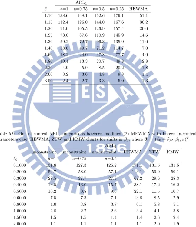
5.9 Out of control ARL comparisons between modified (2) MEWMA with known in-control parameters case, HEWMA, ZTW and KMW charts for shifts in β0, where θj = (β0+ δ0σ, β1, σ)T. . . 37

5.10 Out of control ARL comparisons between modified (2) MEWMA with known in-control parameters case, HEWMA, ZTW and KMW charts for shifts in β1, where θj = (β0, β1+ δ1σ, σ)T. . . 38

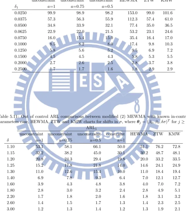
5.11 Out of control ARL comparisons between modified (2) MEWMA with known in-control parameters case, HEWMA, ZTW and KMW charts for shifts in σ, where θj = (β0, β1, δσ)T for j ≥ 1. . . . 38

1

Introduction

1.1

Motivation

Control charts are important monitoring tools used to determine whether a manufac-turing or business process is in a state of statistical control. Roberts (1959) proposed an exponentially weighted moving average (EWMA) control chart which is sensitive to a small shift in the in-control process mean. The likelihood ratio (LR) test is a statistical test used to compare the fit of two models.

Monitoring schemes by an EWMA control chart based on the LR test statistics have been proposed in the literature, e.g., Zou et al. (2006) proposed an EWMA control chart based on LR test statistics for monitoring simple linear profiles with unknown in-control process parameters and Zou et al. (2007) proposed a multivariate EWMA (MEWMA) control chart based on LR test statistics for monitoring general linear pro-files with known in-control process parameters. The LR and score test statistics are asymptotically equivalent under the null hypothesis. Sometimes, it is easier to evaluate the score test statistic than the LR test statistic. The in-control process parameters are usually unknown in practice. We would like to utilize the score test statistics to monitor general linear profiles by an EWMA monitoring scheme, and then to investigate the performance of the proposed methodology.

1.2

Literature Review

Statistical process control (SPC) is often utilized to monitor an industrial process. How to construct a control chart is an important issue in SPC. The control chart is used to determine whether a manufacturing or business process is in a state of statis-tical control.

The control chart can be used in both phases I and II. In phase I, some reference data are collected and analyzed to assess whether they are in control. Then the in-control process parameters and in-control limits are estimated from the in-in-control data identified from those reference data. In phase II, the process is monitored over time to see whether it is in control by using control limits. The average run length (ARL) is usually used to appraise the process performance.

Shewhart (1931) proposed the ¯X control chart which has been used to monitor the

process mean and has good performance for a large sample size or for detecting a large shift in the process mean.

Page (1954) proposed the cumulative sum (CUSUM) control chart whose perfor-mance is better than that of the Shewhart control chart in detecting a small sustained shift in the process mean.

The EWMA control chart was proposed by Roberts (1959) for detecting a small sus-tained shift in the process mean. Its performance for detecting a small sussus-tained shift in the process mean is better than that of the Shewhart control chart. As the in-control

eters and derived its run-length (RL) distribution. Castagliola et al. (2006) reviewed the EWMA control chart for monitoring the process position and variability. Jensen et

al. (2006) reviewed the effect of parameter estimation and proposed some

recommen-dations for future research.

Sometimes, we are interested in the relationship between a response variable and one or more explanatory variables in the process. Kim et al. (2003) proposed a method based on three EWMA control charts, where these three charts were used for different process parameters in simple linear profiles assuming the in-control process parameters are known. Zou et al. (2006) proposed an LR-based control chart for a change-point model to monitor simple linear profiles assuming the in-control process parameters are unknown. Zou et al. (2007) proposed an MEWMA control chart for monitoring general linear profiles assuming the in-control process parameters are known. Zou et al. (2009) compared five control schemes for monitoring the process mean subject to drifts. Zou

et al. (2010) proposed a single chart that integrated the EWMA procedure with the

LR test statistics for monitoring both the process mean and variance. Huang (2012) proposed an EWMA control chart based on LR test statistics for monitoring general linear profiles.

Kim et al. (2003) proposed three EWMA control charts for monitoring simple linear profiles as follows: Suppose that data {(xi, yij) : i = 1, 2, . . . , n} are available at time j = 1, 2, . . . , τ , where xis are not all the same and an out-of-control signal occurs at

where εijs are independent standard normal random variables. Model (1.1) is equivalent

to

y_ij = β0

0+ β10x0i+ σ εij, i = 1, 2, . . . , n, (1.2)

where β0

0 = β0 + β1x, β¯ 10 = β1, and x0i = xi − ¯x with ¯x = Σni=1xi/n. At time j, the

least-squares estimator of β0 0, β10 , and σ2 are b0j = ¯yj, b1j = Σn i=1(xi− ¯x)yij Σn i=1(xi− ¯x)2 , and MSEj = 1 n − 2 n X i=1 (y_ij − b0j − b1jx0i)2,

where ¯yj = Σni=1yi/n. Since b0j, b1j, and MSEj are independent random variables, they

proposed three EWMA control charts

EWMAI(j) = λb0j + (1 − λ)EWMAI(j − 1),

EWMAS(j) = λb1j + (1 − λ)EWMAS(j − 1),

and

EWMAE(j) = max{λ ln(MSEj) + (1 − λ)EWMAE(j − 1), ln(σ2)},

where EWMAI(0) = β00, EWMAS(0) = β10, EWMAE(0) = ln(σ2), and λ is a smoothing

parameter in (0, 1]. Those three EWMA control charts are proposed to monitor β0

profiles as follows: Suppose that data (X, yj) are available at time j = 1, 2, . . . , τ ,

where an out-of-control signal occurs at time τ . The process is called in control at time

j if

y_j = Xβ + σ εj, j = 1, 2, . . . , τ, (1.3)

where y_j is an n × 1 response vector and X is an n × p known model (or design) matrix of rank p (< nj), β = (β0, β1, . . . , βp−1)T is a known in-control p × 1 process regression

parameter vector, σ is a known in-control positive process scale parameter, and εjs are

independent standardized error vectors with εj ∼ Nn(0n×1, In). Set

Zj(β) = ˆ βj− β σ and Zj(σ) = Φ−1 µ Fχ2 n−p µ (n − p)ˆσ2 j σ2 ¶¶ ,

where ˆβj = (XTX)−1XTyj, ˆσj2 = (yj− X ˆβj)T(yj− X ˆβj)/(n − p), Φ−1(·) is the inverse

function of the standard normal cumulative distribution function (c.d.f.), and F_χ2

n−p(·)

is the chi-squared c.d.f. with n − p degrees of freedom. Set Zj ≡ (ZTj(β), Zj(σ))T, a

(p + 1) × 1 random vector. When the process is in control at time j, Zj is multivariate

normally distributed with mean vector 0(p+1)×1 and covariance matrix

Then the MEWMA sequence is defined as

Wj = λZj+ (1 − λ)Wj−1, j = 1, 2, . . . ,

where W0 ≡ 0(p+1)×1 and λ is a smoothing parameter in (0, 1]. An out-of-control signal

occurs at time j if

WjΣ−1Wj > L λ

2 − λ,

where L (> 0) is chosen to achieve a specified in-control ARL.

In Section 2, general linear profiles are described and then an EWMA control chart based on score test statistics is proposed for monitoring general linear profiles. In Section 3, a simulation study is presented to illustrate the proposed methodology. In Section 4, conclusions are given. In Section 5, some potential future works is suggested.

2

An EWMA control chart for monitoring general

linear profiles

In this section, general linear profiles are described and then an EWMA control chart based on score test statistics is proposed for monitoring linear profiles.

2.1

Model

Suppose that data {(yij, xij): i = 1, 2, . . . , nj} are available at time j = 1, 2, . . . , τ ,

where yij is the ith response variable at time j, xij is its corresponding explanatory

variable(s), and an out-of-control signal occurs at time τ . Assume that

yij = βj0u0(xij) + βj1u1(xij) + · · · + βj,p−1up−1(xij) + σjεij, i = 1, 2, . . . , nj, (2.1)

where βj0, βj1, . . . , βj,p−1 are unknown real-valued process regression parameters at time j ; u0(·), u1(·), . . . , up−1(·) are known real-valued functions; σj is an unknown positive

process scale parameter at time j ; and εijs are i.i.d. N(0, 1) standardized errors.

Example 1: Model (2.1) has the form

for simple linear profiles if p = 2 or for polynomial profiles if p ≥ 3. Example 2: Model (2.1) has the form

yij = βj0+ k X u=1 βjuxiju+ k X u=1 βjuux2iju+ X 1≤u<u0_≤k

βjuu0x_ijux_iju0+ σ_jε_ij, i = 1, 2, . . . , n_j,

with xij ≡ (xij1, . . . , xijk)T for quadratic polynomial profiles if k ≥ 2.

For simplicity of notation, model (2.1) is rewritten as

y_j = Xjβj + σjεj, (2.2)

where y_j (≡ (yj1, yj2, ..., yjnj)T) is an nj× 1 response vector at time j, Xj is an known

nj × p model (or design) matrix of full rank p (< nj) at time j, βj

(≡ (βj0, βj1, . . . , βj,p−1)T) is a p × 1 parameter vector of unknown real-valued process

regression parameters at time j, σj is an unknown positive process scale parameter at

time j, and εjs are independent standardized error vectors with εj ∼ Nnj(0nj×1, Inj).

Set θj ≡ (βTj, σj)T (∈ Rp× (0, ∞) ≡ Θ), the process parameter vector at time j. Set θ ≡ (βT_{, σ)}T _{(∈ Θ), the in-control process parameter vector.}

2.2

Known in-control process parameters without constraint

In this subsection, assume that the in-control process parameter vector θ is known. The process is called in control at time j if θj = θ or out of control at time j if θj 6= θ.

f (y_j; θj) = 1 (2π)nj/2σnj j exp ½ −kyj − Xjβjk 2 2σ2 j ¾ = 1 (2π)nj/2σnj j exp ( −( ˆβj− βj) T_XT j Xj( ˆβj − βj) + njσˆ2j 2σ2 j ) ,

where ( ˆβT_j, ˆσj)T (≡ ˆθj) is the maximum likelihood estimator (MLE) of θj such that ˆβj

is independent of ˆσj with ˆ β_j ≡ (XT j X)−1j XjTyj ∼ Np(βj, σ2j(XjTXj)−1) (2.3) and ˆ σ2_j ≡ kyj− Xjβˆjk 2 nj = ° °£_In j− Xj(XjTXj)−1XjT ¤ y_j°°2 nj ∼ σ 2 j nj χ2_nj−p. (2.4)

Then the log-likelihood function for θj at time j is

`j(θj) ≡ log £ f (y_j; θj) ¤ = −nj 2 log(2π) − nj 2 log(σ 2 j) − ky_j − Xjβjk2 2σ2 j .

The corresponding LR and score test statistics at time j are

2 h `j( ˆθj) − `j(θ) i and ∂`j(θj) ∂θT j Cov−1 θj µ ∂`j(θj) ∂θj ¶ ∂`j(θj) ∂θj ¯ ¯ ¯ ¯ ¯ θj=θ (≡ Wj),

respectively, where ∂`j(θj)/∂θj is the score function for θj at time j such that ∂`j(θj) ∂β_j = XT j (yj− Xjβj) σ2 j ∼ Np à 0p×1, XT j Xj σ2 j ! , ∂`j(θj) ∂σj = kyj − Xjβjk 2 σ3 j −nj σj ∼ χ 2 nj− nj σj , and ∂`j(θj)/∂βj is independent of ∂`j(θj)/∂σj.

When the process is in control at time j,

2 h `j( ˆθj) − `j(θ) i = Wj+ Op µ 1 √ nj ¶ (2.5)

as nj → ∞, where equation (2.5) is sketched in Appendix A.1.

Wj = ( ˆβ_j − β)T_XT j Xj( ˆβj − β) σ2 + 1 2nj " ( ˆβ_j− β)T_XT j Xj( ˆβj− β) σ2 + njσˆj2 σ2 − nj #₂ ≡ Hj1+ 1 2nj (Hj1+ Hj2− nj)2, (2.6)

where Hj1 is independent of Hj2 such that

Hj1 ≡ ( ˆβ_j − β)T_XT j Xj( ˆβj − β) σ2 ∼ σ2 j σ2χ 2 p((βj − β)TXjTXj(βj − β)/σ2j) (2.7) and Hj2 ≡ njσˆ2j σ2 ∼ σ2 j σ2χ 2 nj−p (2.8) with (β_j−β₀)T_XT

χ2 p distribution if (βj− β0)TXjTXj(βj− β0)/σj2 > 0. Set τ2 j ≡ (β_j − β)T_XT j Xj(βj − β) σ2 j (≥ 0).

Note that the distribution of Wj depends only on all of p, nj, σj/σ, and τj2. When the

process is in control at time j, the distribution of Wj depends only on both p and nj.

Set ¯ Wj ≡ Wj − Eθj(Wj)|θj=θ p Varθj(Wj)|θj=θ , (2.9) where both Eθj(Wj)|θj=θ and Varθj(Wj)|θj=θ are given in Appendix A.2.

2.3

Known in-control process parameters with constraint

In this subsection, assume that the in-control process parameter vector θ is known. In practice, If the process had not been adjusted, the positive scale parameter σj at

time j should not be smaller than in-control σ. When out of control signal occurs, σj

should be larger than the in-control process parameter σ. Therefore, in this subsection, the process is called in control at time j if θj = θ or out of control at time j if θj 6= θ

and σj ≥ σ . The corresponding LR test statistic at time j is

2£`j(θ∗j) − `j(θ) ¤ = 2 h `j( ˆθj) − `j(θ) i − 2 h `j( ˆθj) − `j(θ∗j) i ,

where ˆθj(= ( ˆβj, ˆσj)) is given in subsection 2.2 and θj∗(≡ (β∗Tj , σ∗j)T = ( ˆβ T

j, max{ˆσj, σ})T)

is the corresponding MLE of θj. The corresponding score test statistic is

W_j∗ ≡ ∂`j(θj) ∂θT j Cov−1<sub>θj</sub> µ ∂`j(θj) ∂θj ¶ ∂`j(θj) ∂θj ¯ ¯ ¯ ¯ ¯ θj=θ − ∂`j(θj) ∂θT j Cov−1_θj µ ∂`j(θj) ∂θj ¶ ∂`j(θj) ∂θj ¯ ¯ ¯ ¯ ¯ θj=θj∗ ≡ Wj− Wj(θ∗j), (2.10)

where Wj is given in subsection 2.2 and

Wj(θ∗j) ≡ ∂`j(θj) ∂θT j Cov−1 θj µ ∂`j(θj) ∂θj ¶ ∂`j(θj) ∂θj ¯ ¯ ¯ ¯ θj=θ∗j = nj 2 · min µ Hj2 nj , 1 ¶ − 1 ¸₂

with Hj2 being given in subsection 2.2. Then

W_j∗ = Hj1+ 1 2nj (Hj1+ Hj2− nj)2− nj 2 · min µ Hj2 nj , 1 ¶ − 1 ¸₂ , (2.11)

where Hj1 is given in subsection 2.2. Note that the distribution of Wj∗ depends only on

all of p, nj, σj/σ0, and τj2, where τj2 is given in subsection 2.2. When the process is in

control at time j, the distribution of W∗

j depends only on both p and nj. Set

¯ W_j∗ ≡ W ∗ j − Eθj(Wj∗)|θj=θ q Varθj(Wj∗)|θj=θ , (2.12) where both Eθj(W ∗ j)|θj=θ and Varθj(W ∗

2.4

Unknown in-control process parameters without constraint

In this subsection, assume that the in-control process parameter vector θ is un-known. Assume that the historical in-control process data {X0, y0} are available. The

relationship between y₀ and X0 is assumed to be

y₀ = X0β + σ ε0, (2.13)

where y₀ is an n0× 1 response vector, X0 is an n0× p known model (or design) matrix

of full rank p (< n0), θ (≡ (βT, σ)T) is a (p + 1) × 1 unknown in-control process

parameter vector, and ε0 is a standardized error vector independent of ε1, ε2, . . ., with

ε0 ∼ Nn0(0n0×1, In0). The process is called in control at time j if θj = θ or out of

control at time j if θj 6= θ.

Then the joint p.d.f. of (yT

0, yTj)T at time j is f (y₀, y_j; θ, θj) = f (y0; θ) · f (yj; θj) = 1 (2π)n0/2σn0 exp ½ −ky0− X0βk 2 2σ2 ¾ · f (y_j; θj) = 1 (2π)n0/2σn0 exp ( −( ˆβ − β) T_XT 0X0( ˆβ − β) + n0σˆ2 2σ2 ) · f (y_j; θj),

where ( ˆβT, ˆσ)T_{(≡ ˆθ) is the MLE of θ, ˆβ is independent of ˆσ with}

and ˆ σ2 _≡ ky0− X0βkˆ 2 n0 = ° °£_In j− Xj(X T 0X0)−1X0T ¤ y₀°°2 n0 ∼ σ 2 n0 χ2 n0−p. (2.15)

The log-likelihood function for (θT, θT_j)T _{at time j is}

`0,j(θ, θj) ≡ log £ f (y<sub>0</sub>; θ) · f (y<sub>j</sub>; θj) ¤ = log [f (y<sub>0</sub>; θ)] + log£f (y<sub>j</sub>; θj) ¤ = −n0 2 log(2π) − n0 2 log(σ 2<sub>) −</sub> ky0− X0βk2 2σ2 + `j(θj).

The corresponding LR and score test statistics at time j are

2 h `0,j( ˆθ, ˆθj) − `0,j( ˜θ, ˜θj) i and ∂`0,j(θ, θj) ∂(θT<sub>, θ</sub>T j ) Cov−1 θ,θj µ ∂`0,j(θ, θj) ∂(θ, θj) ¶ ∂`0,j(θ, θj) ∂(θT_{, θ}T j)T ¯ ¯ ¯ ¯ θ= ˜θ,θj= ˜θj (≡ W0,j), where ( ˜θT_{, ˜θ}T

j)T are the MLE of (θT, θTj)T when the process is in control at time j with

˜ β = ˜βj = (X0TX0+ XjTXj)−1(X0Ty0+ XjTyj) =¡XT 0 X0+ XjTXj ¢₋₁³ XT 0X0β + Xˆ jTXjβˆj ´ ˜ σ0 = ˜σj = s ky₀ − X0βk˜ 2+ kyj − Xjβ˜jk2 n0+ nj = s n0σˆ2+ njσˆj2+ ( ˆβ − ˜β)TX0TX0( ˆβ − ˜β) + ( ˆβj − ˜β)TXjTXj( ˆβj− ˜β) n0+ nj s

and ∂`0,j(θ, θj)/∂(θT, θjT)T is the score function for (θT, θTj)T at time j such that ∂`0,j(θ, θj) ∂β = XT 0 (y0− X0β) σ2 ∼ Np µ 0p×1, XT 0X0 σ2 ¶ , ∂`0,j(θ, θj) ∂σ = ky<sub>0</sub>− X0βk2 σ3 − n0 σ ∼ χ2 n0 − n0 σ , ∂`0,j(θ, θj) ∂β_j = XT j (yj− Xjβj) σ2 j ∼ Np à 0p×1, XT j Xj σ2 j ! , ∂`0,j(θ, θj) ∂σj = kyj− Xjβjk 2 σ3 j − nj σj ∼ χ 2 nj − nj σj .

When the process is in control at time j,

2 h `0,j( ˆθ, ˆθj) − `0,j( ˜θ, ˜θj) i = W0,j+ Op à 1 p min{n0, nj} ! , (2.17)

where W0,j = (ˆβ − ˜β)TX0TX0(ˆβ − ˜β) ˜ σ2 + 1 2n0 " (ˆβ − ˜β)T_XT 0X0(ˆβ − ˜β) ˜ σ2 + n0σˆ2 ˜ σ2 − n0 #₂ +(ˆβj − ˜βj) T_XT j Xj(ˆβj− ˜βj) ˜ σ2 j + 1 2nj " (ˆβ_j − ˜β_j)T_XT j Xj(ˆβj − ˜βj) ˜ σ2 j + njσˆ 2 j ˜ σ2 j − nj #₂ = (n0+ nj)( ˆβj − ˆβ) T_A 0j( ˆβj− ˆβ) n0σˆ2+ njσˆj2+ ( ˆβj − ˆβ)TA0j( ˆβj− ˆβ) + 1 2n0    (n0+ nj) h ( ˆβj− ˆβ)TXjTXjB0jX0TX0B0jXjTXj( ˆβj − ˆβ) + n0σˆ2 i n0σˆ2+ njσˆ2j + ( ˆβj− ˆβ)TA0j( ˆβj − ˆβ) − n0    2 + 1 2nj    (n0+ nj) h ( ˆβj − ˆβ)TX0TX0B0jXjTXjB0jX0TX0( ˆβj − ˆβ) + njσˆ2j i n0σˆ2+ njσˆj2+ ( ˆβj − ˆβ)TA0j( ˆβj − ˆβ) − nj    2 with A0j ≡ [(X0TX0)−1+ (XjTXj)−1]−1 and B0j ≡ (X0TX0+ XjTXj)−1.

When the process is in control at time j, the distribution of W0,j depends only on all

of p, n0, nj and p eigenvalues of (X0TX0)−1/2XjTXj(X0TX0)−1/2. Set

¯ W0,j ≡ W0,j − Eθ,θj(W0,j)|θ=˜θ,θj=˜θj q Varθ,θj(W0,j)|θ=˜θ,θj=˜θj , (2.18)

where both Eθ,θj(W0,j)|θ=˜θ,θj=˜θj and Varθ,θj(W0,j)|θ=˜θ,θj=˜θj do not depend on the

un-known in-control process parameter vector θ and are given in Appendix C.1.

2.5

Unknown in-control process parameters with constraint

In this subsection, assume that the in-control process parameter vector θ is unknown. And the positive scale parameter σj at time j (j ≥ 1) is larger than or equal to the

in-control process parameter σ if the process has not been adjusted until time j. Therefore, in this subsection, the process is called in control at time j if θj = θ or out of control

at time j if θj 6= θ and σj ≥ σ . The corresponding LR test statistic at time j is

2 h `0,j(θ∗, θj∗) − `0,j( ˜θ, ˜θj) i = 2 h `0,j( ˆθ, ˆθj) − `0,j( ˜θ, ˜θj) i − 2 h `0,j( ˆθ, ˆθj) − `0,j(θ∗, θj∗) i

where ˆθ, ˆθj, ˜θ, and ˜θj are given in subsection 2.3, (θ∗, θj∗) (≡ (β∗, σ∗, βj∗, σj∗)) are

the MLE of (θ, θj) under out-of-control status with

β∗ _{= ˆβ, σ}∗ _{= ˆσ · 1} {ˆσj≥ˆσ}+ s ky0− X0βkˆ 2+ kyj − Xjβˆjk2 n0+ nj · 1{ˆσj<ˆσ},

and β∗_j = ˆβj, σj∗ = ˆσj· 1{ˆσj≥ˆσ}+ s ky0− X0βkˆ 2+ kyj − Xjβˆjk2 n0+ nj · 1{ˆσj<ˆσ}.

The corresponding score test statistic is

W_0,j∗ ≡ W0,j − W0,j(θ∗, θj∗),

where W0,j is given in subsection 2.4, and

W0,j(θ∗, θj∗) ≡ ∂`0,j(θ, θj) ∂(θT<sub>, θ</sub>T j) Cov−1 θ,θj µ ∂`0,j(θ, θj) ∂(θ, θj) ¶ ∂`0,j(θ, θj) ∂(θT_{, θ}T j )T ¯ ¯ ¯ ¯ θ=θ∗_,θ j=θ∗j = n0 2 µ ˆ σ2 σ∗2 − 1 ¶2 + nj 2 µ ˆ σ2 j σ∗2 j − 1 ¶2 = (n0 + nj) ³n0nj 2 ´ µ _σˆ2 _{− ˆσ}2 j n0σˆ2+ njσˆ2j ¶2 · 1{ˆσj<ˆσ}. (2.19) When the process is in control at time j, the distribution of W∗

0,j depends only on p, n0, and nj. Set ¯ W_0,j∗ ≡ W ∗ 0,j − Eθ,θj(W0,j∗ )|θ=˜θ,θj=˜θj q Varθ,θj(W0,j∗ )|θ=˜θ,θj=˜θj , (2.20) where both Eθ,θj(W ∗ 0,j)|θ=˜θ,θj=˜θj and Varθ,θj(W ∗

0,j)|θ=˜θ,θj=˜θj are given in Appendix D.1.

2.6

Proposed monitoring scheme

The EWMA sequence is defined as 

  

where λ is a smoothing parameter in (0, 1], and ˜Wj = ¯Wj in subsection 2.2, or ˜Wj = ¯Wj∗

in subsection 2.3, ˜Wj = ¯W0,j in subsection 2.4, ˜Wj = ¯W0,j∗ in subsection 2.5. Then,

standardize the statistic and define the control chart statistic as

U∗ j ≡ U_pj − Eθ(Uj) Varθ(Uj) , (2.22) where Eθ(Uj) = 0, and Varθ(Uj) = λ [1 − (1 − λ) 2j_] 2 − λ , for known θ case;

Eθ(Uj) = 0, and Varθ(Uj) = λ [1 − (1 − λ)2j_] 2 − λ + 2λ 2 X 0≤k1<k2≤j−1 (1 − λ)k1+k2_{Cov( ˜W} j−k1, ˜Wj−k2),

for unknown θ case. Because ˜Wj−k1 and ˜Wj−k2 are correlative, so the calculation of

here recommend X0 and Xj as X0 =           X ... X           (mn)×p , Xj =           X ... X           (mjn)×p , j ≥ 1,

where X is a n×p design matrix, then Cov( ˜Wj−k1, ˜Wj−k2) will only depend on n, p, m, mj−k1, mj−k1

Out-of-control signal occurs at time j if

U∗ j > C,

where C > 0 is chosen by a specified in-control ARL (≡ ARL0). C only depend on

ARL0, λ, p, n1, n2, . . . for known θ case and depend on ARL0, λ, p, n, m, m1, m2, . . .

3

A Simulation Study

In this Section, we explain how to simulate the proposed EWMA control chart for comparison with the Kim et al. (2003) and Zou et al. (2007). Consider the case of constrained EWMA control chart with known parameters first. If the process is in control, in equation (2.11), the Hj1 follows chi-squared distribution with p degrees of

freedom, Hj2 follows chi-squared distribution with nj− p degrees. Use this property to

generate test statistic and find control limit C.

Step 1 : Choose the specific ARL0 and smoothing parameter λ, here given ARL0=200

and λ=0.2 and 50,000 simulations, The same assumptions with Kim et al. (2003) and Zou et al. (2006)

Step 2 : Generate 200 Hj1 and Hj2, and calculated 200 Wj∗, Uj, and Uj∗, for j =

1, 2, . . . , 200

Step 3 : c ≡ max{U∗

1, U2∗, . . . , U200∗ } .

Step 4 : Repeat Step (2) ∼ Step (3) 50,000 times, obtain 50,000 c, and make them to sort (c(1) < c(2) < . . . < c(50000)).

Step 5 : Choose the median of the 50,000 c as the control limit. Use this control limit, make 50,000 time simulation, then obtain 50,000 Run Length, and compute the ARL. Step 6 : Use bisection method if the ARL > 200 then make control limit as the smaller

It can be easily generate the out-of-control W∗

j by equation (2.11), and use the

con-trol limit which obtained previously to calculate the out-of concon-trol ARL (ARL1) with

50,000 simulations.

Next, consider the case of constrained EWMA control chart with unknown param-eters. The procedure is same as case of constrained EWMA control chart with known parameters except the generation of U∗_{. In subsection 2.5, W}∗

0,j consists of ˆβ, ˆβj, ˆσ, and ˆσj, where ˆ β ∼ Np(β, σ2(X0TX0)−1), ˆ βj ∼ Np(βj, σj2(XjTXj)−1), ˆ σ ∼ σ2_/n 0χ2n0−p, ˆ σj ∼ σj2/njχ2nj−p,

and they are independent respectively. W∗

0,j and W0,j∗ 0 are depends on p, n₀, n₁, . . .(j 6=

j0_{), and therefore the X}

0 and Xj must be design matrix. Then generate U∗ through

above property.

We consider the case from Kim et al. (2003) and Zou et al. (2007), the simplest case of model (2.2) with p = 2, in-control parameters β ≡ (β0, β1)T = (3, 2)T, σ = 1, fixed

Xj, Xj ≡ X =               1 2 1 4 1 6 1 8               , j ≥ 1, and X0 =           X ... X           4m×p .

4

Conclusions

4.1

Monitoring performance comparisons

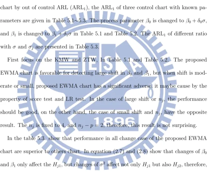
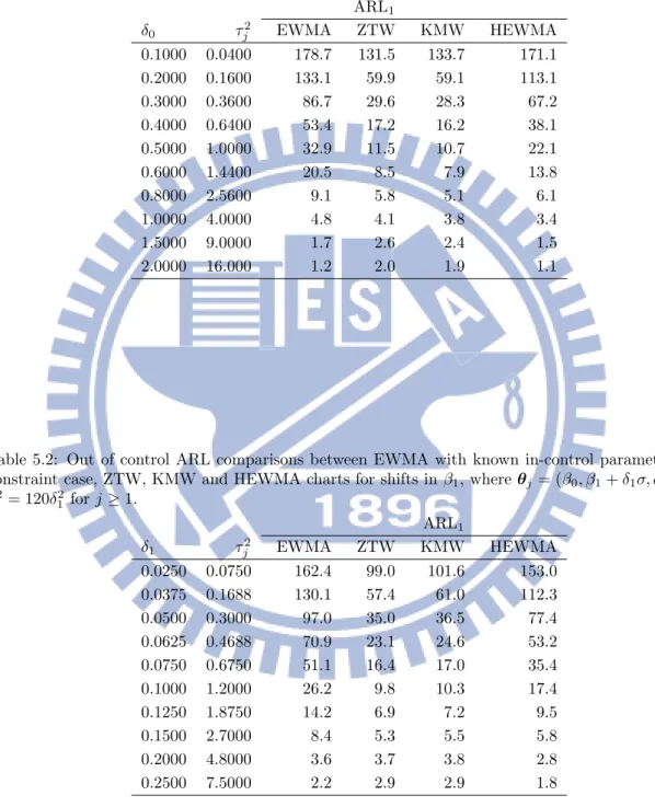
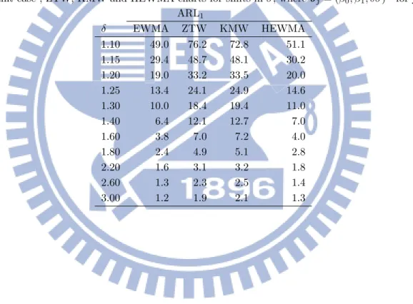
Compared proposed EWMA chart with the KMW, ZTW and Huang (2012) EWMA chart by out of control ARL (ARL1), the ARL1 of three control chart with known

pa-rameters are given in Table 5.1∼5.3. The process parameter β0 is changed to β0+ δ0σ,

and β1 is changed to β1+ δ1σ in Table 5.1 and Table 5.2. The ARL1 of different ratio

with σ and σj are presented in Table 5.3.

First focus on the KMW and ZTW, In Table 5.1 and Table 5.2. The proposed EWMA chart is favorable for detecting large shift in β0 and β1, but when shift is

mod-erate or small, proposed EWMA chart has a significant adverse, it maybe cause by the property of score test and LR test. In the case of large shift or nj, the performance

should be good, on the other hand, the case of small shift and nj, have the opposite

result. The nj is fixed to 4, and nj − p = 2, therefore, this result is not surprising.

In the table 5.3. show that performance in all change case of the proposed EWMA chart are superior to others chart. In equation (2.7) and (2.8) show that changes of β0

and β1only affect the Hj1, but changes of σ2 affect not only Hj1 but also Hj2, therefore,

the proposed EWMA chart is more sensitive when σ2 _shifted.

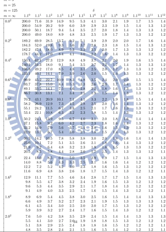
Table 5.4 presented ARL1 with process parameters β and σ change

rameters case.

4.2

Modify monitoring scheme (1)

In Huang (2012), he proposed an EWMA control chat based on LR test statistic, it is similar with the method we proposed. It should be similar results in theory, but according to Table 5.1∼5.3, they are a little difference. The HEWMA is better than proposed EWMA when the β shifted, and it is worse than proposed EWMA when the

σ shifted.

Here proposed an improved method, we transform the score statistic to make it more sensitive for the detection of β.

Wj = ( ˆβ_j− β)T_XT j Xj( ˆβj− β) σ2 0 +a " Φ−1 à Fχ2 nj à ( ˆβ_j − β)T_XT j Xj( ˆβj − β) σ2 + njσˆ2j σ2 !!#₂ ,

for two-sided case, and

W∗ j = ( ˆβ_j − β)T_XT j Xj( ˆβj − β) σ2 +aF_χ−12 1 à Fχ2 nj à ( ˆβ_j− β)T_XT j Xj( ˆβj− β) σ2 + njσˆj2 σ2 !! ,

detection of β, and therefore the ARL1 performance with 0 < a < 1 are given in Table

5.6 and Table 5.7. When a the smaller, the performance will be almost the same as with the HEWMA or better. We found very bad performance for the detection of σ shifted in table 5.8. When the emphasis on the sift of β, we recommend the use this method, and when the emphasis on the shift of σ, we recommend using the methods mentioned earlier.

4.3

Modify monitoring scheme (2)

In the previous subsection, even the use of the modified statistic β shifted ARL1

performance still worse than KMW and ZTW. And think it is ( ˆβ_j − β)T_XT

j Xj( ˆβj − β)/σ2 _{terms caused. It makes all the factors of β changes into a single value. Then}

propose a improve method. First use the MEWMA Chart. Let

W0 ≡ 0p+1×1 Wj ≡           Wj1 ... Wj,p+1           = λ      ∂`j/∂βj|θj=θ Φ−1³<sub>F</sub> ∂`j/∂σj|_{θj =θ} ¡ ∂`j/∂σj|θj=θ; θ ¢´     + (1 − λ)Wj−1, j = 1, 2, 3, · · · , = λ      XT j (yj− Xjβ)/σ2 Φ−1³_F χ2 nj (kyj − Xjβk 2_/σ2₎´     + (1 − λ)Wj−1, j = 1, 2, 3, · · · , (4.1)

where XT

j (yj− Xjβ)/σ2 and Φ−1

³

Fχ2

nj (kyj − Xjβk

2_/σ2₎´_{are not independent but}

Covθj=θ ³ X_jT(yj− Xjβ)/σ2, Φ−1 ³ Fχ2 nj ¡ kyj − Xjβk2/σ2 ¢´´ = 0p×1, and Covθ1,...,θj(Wj) ¯ ¯ θ1=...=θj=θ = λ 2 j X k=1 (1 − λ)2(j−k)      XT kXk/σ2 0p×1 0T p×1 1     , j = 1, 2, . . . .

Then make the two-sided score test statistic as

Uj =           Wj1 ... Wjp           T Cov−1           Wj1 ... Wjp           ¯ ¯ ¯ ¯ ¯ ¯ ¯ ¯ ¯ ¯ ¯ ¯ ¯ ¯ θ1=...=θj=θ           Wj1 ... Wjp           + a W 2 j,p+1 λ2Pj k=1(1 − λ)2(j−k) , (4.2) and the one-sided score test statistic as

U∗ j =           Wj1 ... Wjp           T Cov−1           Wj1 ... Wjp           ¯ ¯ ¯ ¯ ¯ ¯ ¯ ¯ ¯ ¯ ¯ ¯ ¯ ¯ θ1=...=θj=θ           Wj1 ... Wjp           + aF−1 χ2 1  Φ   Wj,p+1 λqPj_k=1(1 − λ)2(j−k)     , (4.3) where a ∈ (0, ∞). Similar with before, the greater a is, and the more sensitive for the

In table 5.9 and table 5.10 shows the simulation results of the β shifted with two-sided case. The ARL1 performance of the improve method is very close with ZTW and

KMW, and when the constant a is getting smaller even better than their. In table 5.11 shows the simulation results of the σ shifted with two-sided and one-sided case. When constant a = 1, one-sided case more sensitive than two-sided, and the they are better than ZTW and KMW, but slightly worse than HEMWA. And the greater constant a is, the worse performance becomes. This improve method can be seen here in the case of whether β shifted or σ shifted has good, and to focus on detection of shifts in the β or σ by by adjusting constant a.

5

Future Work

In this paper, the MEWMA performance seems better than the performance of EWMA based on score test statistics. In future work, it can focus on MEWMA. Con-sider the nonlinear model. e.g., yj = uj(Xj; βj) + σjεj, where uj(· ; ·) is a known

function for j = 1, 2, · · · . May also consider the error term is not a normal distribution. e.g., t-distribution. And considered the MEWMA method based on score test statistics will have a good performance.

References

[1] Castagliola, P., Celano, G., and Fichera, S. (2006) Monitoring process variability using EWMA. Springer Handbook of Engineering Statistics, 291-325. Ch.17. [2] Huang, W-C. (2012) An exponentially weighted moving average control chart based

on likelihood ratio test statistics for monitoring general linear profiles. Master the-sis, National Chiao Tung University, Hsinchu, Taiwan.

[3] Jensen, W. A., Champ, C. W., and Woodall, W. H. (2006) Effects of parameter estimation on control chart properties: a literature review. Journal of Quality

Technology, 38, 156-167.

[4] Jones, L. A., Champ, C. W., and Rigdon, S. E. (2001) The performance of exponen-tially weighted moving average charts with estimated parameters. Technometrics, 43, 156-167.

[5] Kim, K., Mahmoud, M., and Woodall, W. H. (2003) On the monitoring of linear profiles. Journal of Quality Technology, 35, 317-328.

[6] Kots, Balakrishnan and Johnson. (2000) Continuous multivariate distributions vol-ume 1 second edition.

[9] Shewhart, W. A. (1931) Economic control of quality of manufactured product, American Society for Quality, Vol. 509.

[10] Zou, C., Lin, Y., and Wang, Z. (2009) Comparisons of control schemes for moni-toring the means of processes subject to drifts. Metrika, 70, 141-163.

[11] Zou, C., Tsung, F., and Wang, Z. (2007) Monitoring general linear profiles using multivariate exponentially weighted moving average schemes. Technometrics, 49, 395-408.

[12] Zou, C., Zhang, Y., and Wang, Z. (2006) A control chart based on a change-point model for monitoring linear profiles. Transactions, 38, 1093-1103.

[13] Zou, C., Zhang, J., and Wang, Z. (2010) A control chart based on likelihood ratio test for monitoring process mean and variability. Quality and Reliability

Table 5.1: Out of control ARL comparisons between EWMA with known in-control parameters and constraint case, ZTW, KMW and HEWMA charts for shifts in β0, where θj = (β0+ δ0σ, β1, σ)T and

τ2 j = 4δ20 for j ≥ 1. ARL1 δ0 τj2 EWMA ZTW KMW HEWMA 0.1000 0.0400 178.7 131.5 133.7 171.1 0.2000 0.1600 133.1 59.9 59.1 113.1 0.3000 0.3600 86.7 29.6 28.3 67.2 0.4000 0.6400 53.4 17.2 16.2 38.1 0.5000 1.0000 32.9 11.5 10.7 22.1 0.6000 1.4400 20.5 8.5 7.9 13.8 0.8000 2.5600 9.1 5.8 5.1 6.1 1.0000 4.0000 4.8 4.1 3.8 3.4 1.5000 9.0000 1.7 2.6 2.4 1.5 2.0000 16.000 1.2 2.0 1.9 1.1

Table 5.2: Out of control ARL comparisons between EWMA with known in-control parameters and constraint case, ZTW, KMW and HEWMA charts for shifts in β1, where θj = (β0, β1+ δ1σ, σ)T and

τ2 j = 120δ12 for j ≥ 1. ARL1 δ1 τj2 EWMA ZTW KMW HEWMA 0.0250 0.0750 162.4 99.0 101.6 153.0 0.0375 0.1688 130.1 57.4 61.0 112.3 0.0500 0.3000 97.0 35.0 36.5 77.4 0.0625 0.4688 70.9 23.1 24.6 53.2 0.0750 0.6750 51.1 16.4 17.0 35.4 0.1000 1.2000 26.2 9.8 10.3 17.4 0.1250 1.8750 14.2 6.9 7.2 9.5 0.1500 2.7000 8.4 5.3 5.5 5.8 0.2000 4.8000 3.6 3.7 3.8 2.8 0.2500 7.5000 2.2 2.9 2.9 1.8

Table 5.3: Out of control ARL comparisons between EWMA with known in-control parameters and constraint case , ZTW, KMW and HEWMA charts for shifts in σ, where θj = (β0, β1, δσ)T for j ≥ 1.

ARL1 δ EWMA ZTW KMW HEWMA 1.10 49.0 76.2 72.8 51.1 1.15 29.4 48.7 48.1 30.2 1.20 19.0 33.2 33.5 20.0 1.25 13.4 24.1 24.9 14.6 1.30 10.0 18.4 19.4 11.0 1.40 6.4 12.1 12.7 7.0 1.60 3.8 7.0 7.2 4.0 1.80 2.4 4.9 5.1 2.8 2.20 1.6 3.1 3.2 1.8 2.60 1.3 2.3 2.5 1.4 3.00 1.2 1.9 2.1 1.3

Table 5.4: ARLs with unknown in-control parameters and constraint case for shifts in θ with θj = (βT_j, δσ)T _{and τ}2 j = τ2/δ2for j ≥ 1 m = 5 m = 25 m = 125 δ m = ∞ 1.10 _1.11 _1.12 _1.13 _1.14 _1.15 _1.16 _1.17 _1.18 _1.19 _1.110 _1.111 _1.112 0.02 _{200.0 71.6 31.9 14.9 9.5 5.3 4.1 3.0 2.1 1.9 1.7 1.5 1.4} 200.0 54.9 20.2 9.9 6.0 3.9 2.9 2.3 1.9 1.5 1.4 1.3 1.2 200.0 50.1 18.7 9.4 5.4 3.5 2.7 2.0 1.8 1.4 1.3 1.3 1.2 200.0 49.0 18.0 8.9 4.8 3.3 2.5 1.9 1.7 1.3 1.3 1.2 1.2 0.22 _{189.2 69.9 28.5 13.7 9.2 5.1 3.9 2.9 2.0 2.0 1.7 1.6 1.4} 184.3 52.0 19.8 9.3 5.6 3.7 2.8 2.3 1.8 1.5 1.4 1.3 1.2 182.2 47.1 18.0 8.9 5.3 3.2 2.5 2.0 1.7 1.3 1.3 1.2 1.2 178.7 44.2 17.0 8.4 4.1 3.0 2.2 1.6 1.4 1.3 1.3 1.2 1.2 0.42 _{150.1 62.1 27.3 12.9 8.8 4.9 3.7 2.7 2.0 1.9 1.6 1.5 1.4} 140.1 54.3 18.0 9.1 5.4 3.5 2.7 2.2 1.7 1.4 1.3 1.3 1.2 136.8 49.2 17.0 8.5 4.8 3.1 2.5 2.0 1.7 1.3 1.3 1.2 1.2 133.1 40.1 14.1 7.9 3.9 2.6 2.0 1.5 1.4 1.3 1.3 1.2 1.2 0.62 _{99.9 45.2 22.7 10.9 8.3 4.8 3.5 2.4 2.0 2.0 1.5 1.5 1.4} 93.7 37.8 15.0 8.4 5.3 3.3 2.6 2.0 1.7 1.4 1.3 1.2 1.2 89.1 33.5 14.1 7.5 4.6 2.8 2.2 1.8 1.6 1.3 1.3 1.2 1.2 86.7 30.8 13.1 7.1 3.4 2.5 1.9 1.5 1.4 1.3 1.3 1.2 1.2 0.82 _{70.2 43.1 20.9 10.1 7.1 4.1 3.3 2.2 1.9 1.8 1.5 1.4 1.4} 58.2 26.9 12.9 7.3 4.5 2.8 2.5 2.0 1.6 1.4 1.3 1.2 1.2 55.1 24.2 11.5 6.7 3.8 2.5 2.1 1.7 1.6 1.3 1.3 1.2 1.2 53.4 22.1 10.8 6.3 3.2 2.3 1.8 1.5 1.4 1.3 1.3 1.2 1.2 τ2 _1.02 _{50.2 24.1 13.9 9.5 6.7 4.0 3.1 2.0 1.8 1.6 1.4 1.4 1.4} 37.1 15.8 9.2 6.0 4.2 2.7 2.3 1.8 1.6 1.4 1.3 1.2 1.2 33.2 14.9 7.9 5.6 3.7 2.4 2.0 1.6 1.5 1.3 1.3 1.2 1.2 32.9 13.7 6.7 5.4 3.0 2.1 1.8 1.5 1.4 1.3 1.3 1.2 1.2 1.22 _{30.5 14.2 10.5 7.8 5.8 3.8 3.0 2.0 1.8 1.6 1.4 1.4 1.3} 25.6 10.1 7.2 5.1 3.5 2.6 2.1 1.8 1.6 1.4 1.3 1.2 1.2 21.9 9.2 6.4 4.8 3.2 2.3 1.9 1.6 1.5 1.3 1.3 1.2 1.2 20.5 8.5 5.8 4.4 2.8 2.0 1.7 1.5 1.4 1.3 1.3 1.2 1.1 1.42 _{22.4 13.0 8.5 6.4 5.0 3.5 2.9 1.9 1.7 1.5 1.4 1.3 1.3} 14.0 8.8 5.6 4.3 3.3 2.5 2.1 1.6 1.6 1.4 1.2 1.2 1.2 12.2 7.2 5.2 4.2 3.0 2.3 1.8 1.6 1.5 1.3 1.2 1.2 1.2 11.6 6.9 4.8 3.8 2.6 1.8 1.7 1.5 1.4 1.3 1.2 1.2 1.1 1.62 _{12.9 11.1 7.7 5.5 4.6 3.4 2.8 1.7 1.7 1.5 1.4 1.3 1.3} 9.8 5.5 4.7 3.8 3.2 2.4 1.9 1.6 1.5 1.3 1.2 1.2 1.2 9.6 5.3 4.4 3.5 2.9 2.1 1.7 1.8 1.4 1.3 1.2 1.2 1.2 9.1 4.9 4.0 3.3 2.5 1.7 1.6 1.5 1.4 1.3 1.2 1.2 1.1 1.82 _{8.9 6.9 5.4 4.5 3.8 3.0 2.5 1.6 1.5 1.4 1.4 1.3 1.3} 6.6 4.9 3.7 3.2 2.7 2.3 2.1 1.9 1.5 1.3 1.3 1.3 1.2

Table 5.5: ARLs with unknown in-control parameters case for shifts in θ with θj = (βTj, δσ)T and τ2 j = τ2/δ2 for j ≥ 1 m = 5 m = 25 m = 125 δ m = ∞ 1.10 _1.11 _1.12 _1.13 _1.14 _1.15 _1.16 _1.17 _1.18 _1.19 _1.110 _1.111 _1.112 2.22 _{5.4 4.3 3.6 3.3 3.1 2.6 2.4 2.1 1.9 1.8 1.6 1.5 1.3} 4.1 3.6 2.7 2.3 2.2 2.0 1.8 1.7 1.6 1.5 1.4 1.2 1.2 3.8 3.3 2.5 2.3 2.2 1.8 1.7 1.6 1.5 1.4 1.3 1.2 1.1 3.6 3.1 2.4 2.1 1.8 1.7 1.6 1.5 1.3 1.2 1.2 1.2 1.1 2.42 _{4.5 3.8 3.1 2.8 2.6 2.4 2.2 1.8 1.8 1.7 1.5 1.4 1.3} 3.5 3.0 2.2 2.1 2.0 1.7 1.7 1.6 1.5 1.4 1.3 1.2 1.2 3.2 2.9 2.2 2.0 1.9 1.7 1.7 1.5 1.5 1.4 1.3 1.2 1.1 3.0 2.2 2.0 1.9 1.6 1.6 1.6 1.5 1.3 1.2 1.2 1.2 1.1 2.62 _{4.9 3.2 2.9 2.6 2.4 2.3 2.0 1.7 1.7 1.6 1.4 1.3 1.2} 3.2 2.7 2.1 1.9 1.8 1.7 1.6 1.5 1.4 1.3 1.3 1.2 1.2 3.0 2.3 1.9 1.8 1.6 1.6 1.5 1.5 1.3 1.3 1.2 1.2 1.1 2.6 2.0 1.8 1.8 1.5 1.5 1.4 1.4 1.2 1.2 1.2 1.1 1.1 2.82 _{3.5 3.1 2.4 2.2 2.0 2.0 1.9 1.6 1.6 1.5 1.4 1.3 1.2} 2.8 2.1 1.9 1.7 1.6 1.6 1.5 1.4 1.4 1.3 1.2 1.2 1.2 2.4 1.9 1.7 1.6 1.6 1.5 1.5 1.4 1.3 1.3 1.2 1.1 1.1 2.2 1.6 1.5 1.5 1.5 1.4 1.4 1.3 1.3 1.2 1.2 1.1 1.1 3.02 _{3.2 2.9 2.2 2.0 1.9 1.9 1.8 1.6 1.5 1.4 1.3 1.3 1.3} 2.5 1.9 1.7 1.6 1.5 1.4 1.4 1.4 1.3 1.3 1.2 1.2 1.1 2.1 1.8 1.6 1.4 1.4 1.4 1.4 1.3 1.3 1.2 1.2 1.1 1.1 1.8 1.6 1.4 1.4 1.4 1.4 1.3 1.3 1.2 1.2 1.2 1.1 1.1 τ2 _3.22 _{2.9 2.7 2.1 1.9 1.8 1.8 1.7 1.5 1.5 1.4 1.3 1.3 1.3} 2.1 1.9 1.6 1.5 1.5 1.4 1.4 1.3 1.3 1.2 1.2 1.2 1.1 1.9 1.7 1.5 1.4 1.4 1.4 1.3 1.3 1.2 1.2 1.1 1.1 1.1 1.7 1.5 1.4 1.4 1.4 1.3 1.3 1.2 1.2 1.2 1.1 1.1 1.1 3.42 _{2.7 2.1 1.9 1.8 1.7 1.7 1.6 1.5 1.5 1.4 1.4 1.3 1.2} 1.8 1.6 1.4 1.3 1.4 1.3 1.3 1.3 1.2 1.2 1.2 1.1 1.1 1.7 1.5 1.3 1.3 1.3 1.3 1.2 1.2 1.2 1.2 1.1 1.1 1.1 1.5 1.4 1.3 1.3 1.3 1.2 1.2 1.2 1.2 1.1 1.1 1.1 1.1 3.62 _{2.0 1.7 1.7 1.7 1.6 1.6 1.5 1.4 1.4 1.3 1.3 1.3 1.2} 1.6 1.5 1.4 1.4 1.3 1.3 1.3 1.2 1.2 1.2 1.2 1.1 1.1 1.5 1.4 1.3 1.3 1.3 1.3 1.2 1.2 1.2 1.2 1.1 1.1 1.1 1.4 1.2 1.2 1.2 1.2 1.2 1.2 1.2 1.1 1.1 1.1 1.1 1.1 3.82 _{1.7 1.6 1.5 1.5 1.5 1.5 1.4 1.4 1.3 1.3 1.2 1.3 1.2} 1.5 1.3 1.3 1.2 1.3 1.2 1.2 1.2 1.2 1.2 1.1 1.1 1.1

Table 5.6: Out of control ARL comparisons between modified (1) EWMA with known in-control parameters case and HEWMA charts for shifts in β0, where θj = (β0+ δ0σ, β1, σ)T and τj2= 4δ02 for

j ≥ 1.

ARL1

δ0 τj2 a=1 a=0.75 a=0.5 a=0.25 HEWMA

0.1000 0.0400 174.9 173.2 171.8 170.2 171.1 0.2000 0.1600 118.9 117.3 115.8 112.1 113.1 0.3000 0.3600 71.4 69.7 68.5 67.1 67.2 0.4000 0.6400 40.4 39.5 38.9 38.1 38.1 0.5000 1.0000 23.7 23.0 22.5 21.9 22.1 0.6000 1.4400 14.4 14.1 13.7 13.4 13.8 0.8000 2.5600 6.5 6.4 6.2 6.1 6.1 1.0000 4.0000 3.6 3.6 3.5 3.4 3.4 1.5000 9.0000 1.6 1.5 1.5 1.5 1.5 2.0000 16.000 1.1 1.1 1.1 1.1 1.1

Table 5.7: Out of control ARL comparisons between modified (1) EWMA with known in-control parameters case and HEWMA charts for shifts in β1, where θj = (β0, β1+ δ1σ, σ)T and τj2 = 120δ12

for j ≥ 1.

ARL1

δ1 τj2 a=1 a=0.75 a=0.5 a=0.25 HEWMA

0.0250 0.0750 153.6 152.4 152.3 152.2 153.0 0.0375 0.1688 115.6 113.8 112.6 112.3 112.3 0.0500 0.3000 81.6 79.9 78.7 77.6 77.4 0.0625 0.4688 55.8 54.5 53.8 52.8 53.2 0.0750 0.6750 37.7 37.3 36.4 35.3 35.4 0.1000 1.2000 18.6 18.0 17.6 17.2 17.4 0.1250 1.8750 10.0 9.7 9.5 9.3 9.5 0.1500 2.7000 6.1 5.9 5.8 5.6 5.8 0.2000 4.8000 2.9 2.8 2.8 2.7 2.8 0.2500 7.5000 1.8 1.8 1.7 1.7 1.8

Table 5.8: Out of control ARL comparisons between modified (1) EWMA with known in-control parameters case and HEWMA charts for shifts in σ, where θj= (β0, β1, δσ)T for j ≥ 1.

ARL1

δ a=1 a=0.75 a=0.5 a=0.25 HEWMA 1.10 138.6 148.1 162.6 179.1 51.1 1.15 112.4 126.0 144.0 167.6 30.2 1.20 91.0 105.5 126.9 157.4 20.0 1.25 73.0 87.6 110.9 145.9 14.6 1.30 59.2 72.7 96.3 135.9 11.0 1.40 38.6 49.7 71.2 114.7 7.0 1.60 18.2 24.0 37.8 77.7 4.0 1.80 10.4 13.3 20.7 49.8 2.8 2.20 4.9 5.9 8.5 20.2 1.8 2.60 3.2 3.6 4.8 9.8 1.4 3.00 2.4 2.7 3.3 5.9 1.3

Table 5.9: Out of control ARL comparisons between modified (2) MEWMA with known in-control parameters case, HEWMA, ZTW and KMW charts for shifts in β0, where θj= (β0+ δ0σ, β1, σ)T.

ARL1

unconstraint unconstraint unconstraint HEWMA ZTW KMW

δ0 a=1 a=0.75 a=0.5

0.1000 131.8 127.3 126.2 171.1 131.5 131.5 0.2000 59.7 58.0 57.1 113.1 59.9 59.1 0.3000 28.5 27.7 27.3 67.2 29.6 28.3 0.4000 16.5 16.0 15.7 38.1 17.2 16.2 0.5000 10.2 9.8 9.6 22.1 11.5 10.7 0.6000 7.5 7.3 7.1 13.8 8.5 7.9 0.8000 4.0 3.8 3.7 6.1 5.8 5.1 1.0000 2.8 2.7 2.6 3.4 4.1 3.8 1.5000 1.5 1.5 1.4 1.4 2.6 2.4

Table 5.10: Out of control ARL comparisons between modified (2) MEWMA with known in-control parameters case, HEWMA, ZTW and KMW charts for shifts in β1, where θj= (β0, β1+ δ1σ, σ)T.

ARL1

unconstraint unconstraint unconstraint HEWMA ZTW KMW

δ1 a=1 a=0.75 a=0.5

0.0250 99.9 98.9 98.2 153.0 99.0 101.6 0.0375 57.3 56.3 55.9 112.3 57.4 61.0 0.0500 34.8 33.9 32.1 77.4 35.0 36.5 0.0625 22.9 22.0 21.5 53.2 23.1 24.6 0.0750 16.0 15.4 15.0 35.4 16.4 17.0 0.1000 8.5 8.2 8.0 17.4 9.8 10.3 0.1250 5.8 5.6 5.2 9.5 6.9 7.2 0.1500 4.5 4.5 4.3 5.8 5.3 5.5 0.2000 2.7 2.6 2.5 2.8 3.7 3.8 0.2500 1.7 1.7 1.6 1.8 2.9 2.9

Table 5.11: Out of control ARL comparisons between modified (2) MEWMA with known in-control parameters case, HEWMA, ZTW and KMW charts for shifts in σ, where θj = (β0, β1, δσ)T for j ≥ 1.

ARL1

unconstraint unconstraint unconstraint constraint HEWMA ZTW KMW

δ a=1 a=0.75 a=0.5 a=1

1.10 53.1 58.1 66.1 50.0 51.1 76.2 72.8 1.15 32.2 38.2 45.0 30.1 30.2 48.7 48.1 1.20 20.8 24.3 29.4 19.8 20.0 33.2 33.5 1.25 15.2 17.8 21.8 14.0 14.6 24.1 24.9 1.30 11.0 12.6 15.4 10.0 11.0 18.4 19.4 1.40 6.9 7.8 9.3 6.4 7.0 12.1 12.7 1.60 3.9 4.3 4.8 3.8 4.0 7.0 7.2 1.80 2.8 3.0 3.2 2.4 2.8 4.9 5.1 2.20 1.7 1.8 2.0 1.6 1.8 3.1 3.2 2.60 1.4 1.5 1.7 1.3 1.4 2.3 2.5 3.00 1.2 1.3 1.4 1.2 1.3 1.9 2.1

Appendix

A.1

By (A.1), (A.2) and (A.3)

2 h `0<sub>j</sub>( ˆθj) − `0j(θ) i = ( ˆθj − θ)TCovθ(`0j(θ))( ˆθj − θ) + Op µ 1 √ nj ¶ = £`0 j(θ) ¤_T Cov−1 θ ¡ `0 j(θ) ¢ Covθ ¡ `0 j(θ) ¢ Cov−1 θ ¡ `0 j(θ) ¢ `0 j(θj) + Op µ 1 √ nj ¶ = Wj+ Op µ 1 √ nj ¶ .

A.2

When the process is in control,

Hj1 ∼ χ2p and Hj2 ∼ χ2nj−p. Eθ(Wj) = Eθ(Hj1+ 1 2nj (Hj1+ Hj2− nj)2) = p + Var(Hj1+ Hj2) 2nj = p + 1. Varθ(Wj) = 1 4n2 j Eθ ¡ (H_j12 + H_j22 + 2Hj1Hj2− 2njHj2+ n2j)2 ¢ − (p + 1)2 = 1 4n2 j Eθ(Hj14 + Hj24 + 6Hj12 Hj22 + 4Hj13 Hj2+ 4Hj1Hj23 − 4njHj12 Hj2− 8njHj1Hj22 −4njHj23 + 2n2jHj12 + 6n2jHj22 + 4n2jHj1Hj2− 4n3jHj2+ n4j) − (p + 1)2 = 1 4n2 j [Eθ(Hj14) + Eθ(Hj24) + 6Eθ(Hj12)Eθ(Hj22) + 4Eθ(Hj13)Eθ(Hj2) +4Eθ(Hj1)Eθ(Hj23) − 4njEθ(Hj12)Eθ(Hj2) − 8njEθ(Hj1)Eθ(Hj22) − 4njEθ(Hj23) +2n2 jEθ(Hj12 ) + 6n2jEθ(Hj22 ) + 4n2jEθ(Hj1)Eθ(Hj2) − 4n3jEθ(Hj2) + n4j ] − (p + 1)2 = 2p +8p nj + 12 nj + 2

where Eθ(Hj1) = p, Eθ(Hj12 ) = p(p + 2), Eθ(Hj13 ) = p(p + 2)(p + 4), Eθ(Hj14 ) = p(p + 2)(p + 4)(p + 6), Eθ(Hj2) = nj − p, Eθ(Hj22 ) = (nj − p)(nj− p + 2), Eθ(Hj23 ) = (nj − p)(nj− p + 2)(nj− p + 4), Eθ(Hj24 ) = (nj − p)(nj− p + 2)(nj− p + 4)(nj − p + 6)

B.1

where Eθ(Wj) = p + 1 from Appendix A.2 and

Eθ0 ¡ Wj(θj∗) ¢ = nj 2 Eθ ÷ min µ Hj2 nj , 1 ¶ − 1 ¸₂! = nj 2 ½ Eθ µ min µ H2 j2 n2 j , 1 ¶¶ − 2Eθ µ min µ Hj2 nj , 1 ¶¶ + 1 ¾ with Eθ µ min µ H2 j2 n2 j , 1 ¶¶ = Z _nj 0 µ x nj ¶₂ f_χ2 nj −p(x)dx + Z _∞ nj 1 · f_χ2 nj −p(x)dx = Z _nj 0 µ x nj ¶₂ · x (nj−p)/2−1· e−x/2 Γ((nj− p)/2) · 2(nj−p)/2 dx + · 1 − Z _nj 0 f_χ2 nj −p(x)dx ¸ = 2 2_Γ((n j − p)/2 + 2) n2 jΓ((nj − p)/2) · Z _nj 0 x(nj−p)/2+2−1· e−x/2 Γ((nj − p)/2 + 2) · 2(nj−p)/2+2 dx + h 1 − F_χ2 nj −p(nj) i = 1 n2 j (nj − p)(nj− p + 2) · Fχ2 nj −p+4(nj) + h 1 − F_χ2 nj −p(nj) i

and Eθ0 µ min µ Hj2 nj , 1 ¶¶ = Z _nj 0 µ x nj ¶ f_χ2 nj −p(x)dx + Z _∞ nj 1 · f_χ2 nj −p(x)dx = Z _nj 0 µ x nj ¶ · x (nj−p)/2−1· e−x/2 Γ((nj − p)/2) · 2(nj−p)/2 dx + · 1 − Z _nj 0 fχ2 nj −p(x)dx ¸ = 2Γ((nj− p)/2 + 1) njΓ((nj − p)/2) · Z _nj 0 x(nj−p)/2+1−1_{· e}−x/2 Γ((nj− p)/2 + 1) · 2(nj−p)/2+1 dx + h 1 − Fχ2 nj −p(nj) i = 1 nj (nj − p) · Fχ2 nj −p+2(nj) + h 1 − F_χ2 nj −p(nj) i .

Varθ(Wj∗) = Varθ(Wj− Wj(θ∗j)) = Varθ(Wj) + Varθ(Wj(θj∗)) − 2Covθ(Wj, Wj(θj∗)),

where Varθ(Wj) is given in Appendix A.2 and

Varθ0(Wj(θ ∗ j)) = n2 j 4 Varθ0 ÷ min µ Hj2 nj , 1 ¶ − 1 ¸₂! = n 2 j 4 Eθ0 ÷ min µ Hj2 nj , 1 ¶ − 1 ¸₄! − n 2 j 4 " Eθ0 ÷ min µ Hj2 nj , 1 ¶ − 1 ¸₂!#2 , with Eθ ÷ min µ Hj2 nj , 1 ¶ − 1 ¸₄! = Eθ µ min µ H4 j2 n4 j , 1 ¶¶ − 4Eθ µ min µ H3 j2 n3 j , 1 ¶¶ + 6Eθ µ min µ H2 j2 n2 j , 1 ¶¶ −4Eθ µ min µ Hj2 nj , 1 ¶¶ + 1.

Here Eθ µ min µ H4 j2 n4 j , 1 ¶¶ = 1 n4 j (nj − p)(nj − p + 2)(nj − p + 4)(nj − p + 6) · Fχ2 nj −p+8(nj) + h 1 − F_χ2 nj −p(nj) i Eθ µ min µ H3 j2 n3 j , 1 ¶¶ = 1 n3 j (nj − p)(nj − p + 2)(nj − p + 4) · Fχ2 nj −p+6(nj) + h 1 − F_χ2 nj −p(nj) i . Finally, Covθ(Wj, Wj(θj∗)) = 1 4Covθ à (Hj1+ Hj2− nj)2, · min µ Hj2 nj , 1 ¶ − 1 ¸₂! = 1 4Covθ à 2Hj1Hj2+ Hj22 − 2njHj2, · min µ Hj2 nj , 1 ¶ − 1 ¸₂! = 1 2Covθ à Hj1Hj2, · min µ Hj2 nj , 1 ¶ − 1 ¸₂! + 1 4Covθ à H_j22, · min µ Hj2 nj , 1 ¶ − 1 ¸₂! −nj 2 Covθ à Hj2, · min µ Hj2 nj , 1 ¶ − 1 ¸₂! ,

where Covθ à Hj1Hj2, · min µ Hj2 nj , 1 ¶ − 1 ¸₂! = Eθ à Hj1Hj2 · min µ Hj2 nj , 1 ¶ − 1 ¸₂! − Eθ(Hj1Hj2) · Eθ ÷ min µ Hj2 nj , 1 ¶ − 1 ¸₂! = p · Eθ à Hj2 · min µ Hj2 nj , 1 ¶ − 1 ¸₂! − p(nj − p) · Eθ ÷ min µ Hj2 nj , 1 ¶ − 1 ¸₂! , Covθ à H_j22, · min µ Hj2 nj , 1 ¶ − 1 ¸₂! = Eθ à H2 j2 · min µ Hj2 nj , 1 ¶ − 1 ¸₂! − Eθ ¡ H2 j2 ¢ · Eθ ÷ min µ Hj2 nj , 1 ¶ − 1 ¸₂! = Eθ à H2 j2 · min µ Hj2 nj , 1 ¶ − 1 ¸₂! −£2(nj− p) + (nj− p)2 ¤ · Eθ ÷ min µ Hj2 nj , 1 ¶ − 1 ¸₂! , Covθ à Hj2, · min µ Hj2 nj , 1 ¶ − 1 ¸₂! = Eθ à Hj2 · min µ Hj2 nj , 1 ¶ − 1 ¸₂! − Eθ(Hj2) · Eθ ÷ min µ Hj2 nj , 1 ¶ − 1 ¸₂! = Eθ à Hj2 · min µ Hj2 nj , 1 ¶ − 1 ¸₂! − (nj − p) · Eθ0 ÷ min µ Hj2 nj , 1 ¶ − 1 ¸₂! .