適用於數位助聽器之10毫秒群延遲且近似於ANSI S1.11 1/3-octave規範的濾波器組

國

立

交

通

大

學

電子工程學系 電子研究所碩士班

碩

士

論

文

適用於數位助聽器之 10 毫秒群延遲且近似於 ANSI

S1.11 1/3-octave 規範的濾波器組

10ms Group Delay Quasi-ANSI S1.11 1/3-Octave Filter

Bank for Digital Hearing Aids

研究生： 莊明勳

指導教授： 劉志尉

適用於數位助聽器之 10 毫秒群延遲且近似於 ANSI S1.11

1/3-octave 規範的濾波器組

10ms Group Delay Quasi-ANSI S1.11 1/3-Octave Filter Bank for

Digital Hearing Aids

研 究 生：莊明勳

Student: Ming-Hsun Chuang

指導教授：劉志尉 博士

Advisor: Dr. Chih-Wei Liu

國 立 交 通 大 學

電子工程學系 電子研究所碩士班

碩士論文

A Thesis

Submitted to Department of Electronics Engineering & Institute of Electronics College of Electrical and Computer Engineering

National Chiao Tung University

In partial Fulfillment of the Requirements for the Degree of Master of Science

in

Electronics Engineering August 2010

Hsinchu, Taiwan, Republic of China

適用於數位助聽器之 10 毫秒群延遲且近似於 ANSI

S1.11 1/3-octave 規範的濾波器組

研究生：莊明勳

指導教授：劉志尉 博士

國立交通大學

電子工程學系 電子研究所碩士班

摘要

由於 ANSI S1.11 1/3-octave 標準中所定義的濾波器組其分頻方式接近人類的聽覺系統， 因此適合用在助聽器的應用上，然而因為其群延遲高且運算複雜度大，現今助聽器中的 濾波器組大多不採用 ANSI S1.11 1/3-octave 的規格。有鑑於此，本篇論文提出一近似於 ANSI S1.11 1/3-octave 濾波器組的設計，藉由對規格作些微的放寬來使群延遲達到 10 毫 秒的規格標準。本篇論文並提出了可以降低和處方之間匹配誤差的方法，使濾波器規格 的放寬只會對助聽器受到些微的影響，助聽器和處方之間最大的誤差從 0dB 上升到了 1.5dB，但仍然小於人耳最小感受度範圍限度的 3dB。此外本篇論文在其演算法及硬體 架構上都進行了最佳化來達到低運算複雜度和低功耗的要求，以適合助聽器的需求。此 濾波器組採用了 IFIR 以及 multirate 的架構以大幅降低運算量。此濾波器組比起傳統的 ANSI S1.11 FIR 濾波器組設計只需要其 7%運算複雜度以及 26%的儲存空間。另外，本 論文同時完成了此濾波器組的硬體架構設計並在 UMC 90 奈米製程下進行實作。根據模 擬的結果，此濾波器組在 24KHz 的取樣頻率下只消耗 104μW 的功率，比起其他群延遲 在 10 毫秒以下並且針對助聽器應用所設計的濾波器組，本論文所提出的濾波器組在相 同的功耗下，可以有更好的處方匹配能力

10ms Group Delay Quasi-ANSI S1.11

1/3-Octave Filter Bank for Digital Hearing

Aids

Student: Ming-Hsun Chuang Advisor: Dr. Chih-Wei Liu

Department of Electronics Engineering Institute of Electronics

National Chiao Tung University

ABSTRACT

The ANSI S1.11 1/3-octave filter bank is popular in many acoustic applications because it matches the human hearing characteristics. However, the long group delay and the high computational complexity limit the usage in hearing aids. A Quasi-ANSI S1.11 18-band 1/3-octave filter bank is proposed to reduce the group delay. With the proposed matching error optimization method, the results show that the filter bank achieve comparable good matching between prescriptions and hearing aid response. The maximum matching error is only slight increase from 0dB to 1.5dB. Besides, the group delay is significantly reduced from 78ms to 10ms compared with the ANSI S1.11 1/3-octave filter bank design in [20]. On the other hand, the complexity-effective filter bank architecture is developed by exploiting the interpolated FIR and multirate processing techniques. Results shows that the proposed algorithm saves about 93% of multiplications and 74% of storage elements compared with a straightforward FIR filter bank. The low-delay complexity-effective 1/3-octave filter bank is implemented in UMC 90nm CMOS technology. The design consumes only 104μW, which is lower then other works in the literatures with group delay small then 10ms.

誌 謝

碩士生涯轉眼即逝，三年來受到許多人的幫助，在此致上最深的感激。 首先誠摯的感謝指導教授劉志尉老師及林泰吉學長，兩位悉心的教導使我在這些年中獲 益匪淺，感謝老師以及學長不厭其煩的指點我正確的方向，才使我得以完成這本論文。 老師對學問的嚴謹更是我學習的典範，其豐富學養以及學者風範都令我受益良多，也使 我在專業知識及研究態度上更臻成熟。特別感謝楊順聰老師、周世傑老師及劉奕汶老 師，謝謝你們在百忙之中，撥冗參與論文口試，並對我的研究給予寶貴的意見，讓此篇 論文更加完備充實。 感謝實驗室的學長們；感謝郭對我研究上的指導以及遇到瓶頸時的一切支援，並在我極 度不安時陪我去台北口試；感謝歐對我待人處事方面的鼓勵與開示；感謝小@讓我有一 個帄穩的工作站可以用；感謝阿圳教我 verilog；感謝強哥每次潑冷水式的指點，讓我知 道邏輯不通之處，有你們的指導與協助才能有今日的成果。 感謝實驗室的夥伴以及學弟妹們；感謝一起奮鬥三年的胖甘，這些年來花了好多時間在 聽我抱怨；感謝胖妞在我肚子餓的時候送來的食物們；感謝安綺每次都可以把在過期臨 界點的食物們吃光；感謝阿捲、阿賢、小鈺、哲偉、宗慶在研究工作上的一切幫忙。有 了你們在每天晚上前往二餐的路上總是很熱鬧。 感謝工三四樓影印室的阿姨，我的每ㄧ本書你都幫我印的很漂亮；感謝布青在實驗室藏 了把 412 的鑰匙，以及不令色的出借高科技用品；感謝所有在我研究期間給予關心與打 氣的好朋友們，真的非常謝謝你們。 最後，謹將本論文獻給爸爸和媽媽等我最親愛的家人。沒有你們的栽培，就沒有今日的 我，希望我的表現沒有讓你們失望。 明勳 謹誌於 新竹 2010 夏

C

ONTENTS

1 INTRODUCTION ... 1

2 BACKGROUND ... 4

2.1 Human hearing system & hearing loss ... 5

2.2 Hearing aids & auditory compensation ... 10

2.3 Considerations for filter bank ... 14

2.4 Related works ... 15

3 LOW-DELAY FILTER BANK DESIGN ... 19

3.1 Quasi-ANSI S1.11 1/3-octave specification ... 20

3.2 Filter coefficient design ... 24

3.3 Minimize the matching-error ... 26

3.4 Result & verifications ... 27

4 IMPLEMENTATION RESULTS ... 37

4.1 Complexity-effective architecture design... 38

4.2 Hardware implementation ... 47

4.3 Result comparisons ... 50

5 CONCLUSIONS ... 52

L

IST OF

F

IGURES

FIGURE 2-1 HUMAN’S HEARING SYSTEM ... 5

FIGURE 2-2 AUDIOGRAM OF TYPICAL HEARING LOSS ... 8

FIGURE 2-3 DECREASED DYNAMIC RANGE ... 9

FIGURE 2-4 AUDIOGRAM & PRESCRIPTION ... 11

FIGURE 2-5 FUNCTION OF AN ADVANCED DIGITAL HEARING AID ... 12

FIGURE 2-6 DIFFERENT TYPES OF FILTER BANKS ... 16

FIGURE 2-7 MATCHING CAPABILITY COMPARISON FOR FOUR TYPES OF FILTER BANK ... 18

FIGURE 3-1 MAGNITUDE RESPONSE LIMITATION IN ANSI S1.11 1/3-OCTAVE STANDARD ... 21

FIGURE 3-2 QUASI-ANSI S1.11 1/3-OCTAVE FILTER BANK DESIGN FLOW ... 23

FIGURE 3-3 (A) MAGNITUDE RESPONSE LIMITATION IN ANSI S1.11 1/3-OCTAVE STANDARD (B) QUASI-ANSI S1.11 1/3-OCTAVE SPECIFICATION ... 24

FIGURE 3-4 PARAMETERS FOR DESIGNING BAND-PASS FILTER ... 25

FIGURE 3-5 FILTER COEFFICIENT DESIGN FLOW ... 25

FIGURE 3-6 MAGNITUDE RESPONSE OF QUASI-ANSI S1.11 1/3-OCTAVE FILTER BANK ... 29

FIGURE 3-7 MAGNITUDE RESPONSE COMPARISON BETWEEN (A) ANSI S1.11 1/3-OCTAVE FILTER BANK (B) QUASI-ANSI S1.11 1/3-OCTAVE FILTER BANK ... 29

FIGURE 3-8 MATCHING RESULT FOR HEARING LOSS DUE TO AGING ... 30

FIGURE 3-9 MATCHING RESULT FOR RISING HEARING LOSS ... 30

FIGURE 3-10 MATCHING RESULT FOR SEVERE FLAT HEARING LOSS ... 31

FIGURE 3-11 MATCHING RESULT FOR MILD HEARING LOSS AT 4 KHZ ... 32

FIGURE 3-12 MATCHING RESULT FOR MILD HEARING LOSS IN WHOLE FREQUENCIES ... 33

FIGURE 3-13 MATCHING RESULT FOR MILD TO MODERATE HEARING LOSS IN LOW FREQUENCIES ... 33

FIGURE 3-14 MATCHING RESULT FOR HEARING LOSS DUE TO AGING ... 34

FIGURE 3-15 MATCHING RESULT FOR HEARING LOSS ... 35

FIGURE 3-16 MATCHING RESULT FOR HEARING LOSS ... 35

FIGURE 4-1 IFIR IMPLEMENTATION OF H(Z) (FREQUENCY DOMAIN) ... 38

FIGURE 4-2 IFIR IMPLEMENTATION OF H(Z) (TIME DOMAIN) ... 39

FIGURE 4-3 EXPLORE THE OPTIMAL L FOR IFIR FILTER IMPLEMENTATION ... 42

FIGURE 4-4 ILLUSTRATIONS OF MULTIRATE IFIR ARCHITECTURE AND NOBLE IDENTITY ... 44

FIGURE 4-5 ILLUSTRATIONS OF MULTIRATE IFIR ARCHITECTURE AND NOBLE IDENTITY ... 45

FIGURE 4-6 OPTIMAL FACTOR OF EACH BAND ... 46

FIGURE 4-7 COMPLEXITY-EFFECTIVE ARCHITECTURE OF FILTER BANK ... 46

FIGURE 4-8 HARDWARE ARCHITECTURE OF THE PROPOSED FILTER BANK ... 48

L

IST OF

T

ABLES

TABLE 2-1 RESEARCHES ON THE DELAY IN HEARING AIDS ... 13

TABLE 3-1 GROUP DELAY & MATCHING ERROR WITH RESPECT TO K ... 28

TABLE 4-1 COMPUTATIONAL COMPLEXITY (MULTIPLICATIONS PER SAMPLE) WITH DIFFERENT L ... 42

TABLE 4-2 COMPLEXITY COMPARISON WITH DIRECTLY IMPLEMENTATION ... 45

TABLE 4-3 COMPLEXITY COMPARISON OF THREE 1/3-OCTAVE FILTER BANK IMPLEMENTATION ... 47

TABLE 4-4 POWER COMPARISONS OF FILTER BANK FOR HEARING AIDS ... 51

1 I

NTRODUCTION

Hearing aids are hearing instruments that are designed to compensate the hearing loss and improve the speech intelligibility for hearing impaired people. Hearing aids compensate the hearing loss and improve the speech intelligibility with the auditory compensation algorithm. More over, the echo cancellation, the noise reduction, and the speech enhancement algorithms are also used to improve the sound quality. The auditory compensation algorithm makes up for the perceptual distortion, such as the raised hearing thresholds and the squeezed hearing dynamic ranges, by performing the frequency-dependent and non-linear amplification on the input sound. Therefore, a hearing aid needs a filter bank to decompose the input signal into different frequency component and then the prescribed gains can be applied to each component to match the prescriptions. For better match the human hearing characteristics and the NAL-NL1 [1] prescription, the 1/3-octave band filter bank is desirable for hearing aids.

However, the long group delay and the high computational complexity limit the usage of 1/3-octave filter bank in hearing aids. Researches have shown that delay more than 15ms can

cause disturbing perception for hearing aid users hearing their own voices [1]. When the delay becomes longer, the hearing impaired may notice an echo effect. And when even longer (more than 40 ms), the auditory information may out of synchronization with the visual information and disturb lip reading. Besides, the hearing aid is a portable device in which the power consumption is a critical concern. So, we must try our best to reduce the computational complexity in the constraint of delay and matching error.

An 18-band 1/3-octave filter bank has been designed and implemented in [20]. This work adopts the ANSI S1.11 standard base on the fact that the mostly used fitting formula NAL-NL1 prescribes the target gains on each 1/3-octave frequencies defined in the ANSI S1.11 standard. As a result, the hearing aid’s magnitude response can have the best capability to match any type of prescriptions by the use of ANSI S1.11 1/3-octave filter bank. The work also makes use of the multistage IFIR and multi-rate techniques to largely reduce the computational complexity (in terms of number of the multiplications per input sample). The complexity-effective architecture saves about 96% of multiplications comparing that with a straightforward FIR filter bank. However, the price this work pay is the long group delay which is up to 78ms and will largely limit the usage of this design. We observe that the unacceptable long group delay is due to the very sharp transition in lower frequency part of ANSI S1.11 1/3-octave bands. Even using the straightforward FIR or IIR to implement the filter bank, there still have group delay up to 27 ms and this can not be shortening further.

The rest of this thesis is organized as follows. Chapter 2 will give an overview on the human hearing system and hearing impairments. The function of a digital hearing aid and the design considerations also described in this chapter. Current related design of filter bank have been surveyed and summarized. In Chapter 3, we propose a quasi-ANSI S1.11 1/3-octave filter bank design to reduce the group delay. With the proposed matching error optimization method, the error only slightly increases. The filter bank results and verifications on various

types of hearing loss are also shown in this chapter. In Chapter 4, we proposed a complexity-effective architecture to implement the filter bank and use some low-power techniques to reduce the power consumption. Then we show the complexity and implementation results by using UMC 90nm CMOS technology. Chapter 5 concludes this thesis and describes the future works.

2 B

ACKGROUND

In this chapter, we firstly review the human hearing system and the problems faced by people with hearing impairment. Secondly, the basic functions of an advanced digital hearing aid are introduced and we focus on the auditory compensation which aims to compensate the hearing loss and maximize the speech intelligibility. It can be done by fitting the hearing aid to match the prescriptions (typically prescribed by the 1/3-octave prescription formula, NAL-NL1). Thirdly, current researches results about the acceptable group delay of hearing aid are surveyed. Finally, we summarize the requirements and challenges to the filter bank for digital hearing aids.

2.1 Human hearing system & hearing loss

2.1.1 Human hearing system

Human’s hearing is an obligatory and sophisticated system which has high sensitivity, sharp frequency tuning, and wide dynamic range. A normal ear is able to distinguish and process acoustic signals varying in large magnitude and frequency range (from twenty to twenty thousand hertz). The ear can detect fine variations in pitch, loudness, and intonation.

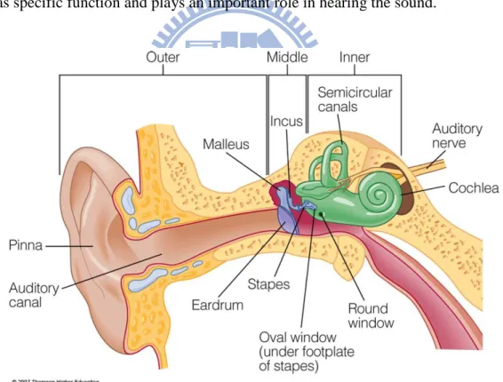
The physical processing of acoustic information occurs in three groups of structures, commonly known as the outer, middle, and inner ears as described in Figure 2-1. Each of them has specific function and plays an important role in hearing the sound.

Figure 2-1 Human’s hearing system

 The outer ear

The outer ear serves to collect the sound, assist in sound localization and function as a protective mechanism for the middle ear. The resonance of the canal favors the high pitches that are important to understand many consonants in the spoken word.

 The middle ear

The middle ear is an air-filled space located within the temporal bone of the skull. It consists of the eardrum and the ossicles (malleus、incus、stapes), linking the membrane to the oval window of the cochlea. Sound pushes the eardrum, thus vibrating the eardrum at the same frequency of the sound wave. The middle ear function as a bridge between the air-borne pressure wave and the fluid-borne traveling of the cochlea.

 The inner ear

The inner ear consists of cochlea, semicircular canals, and the auditory nerve. The inner ear is important for hearing and balance. The cochlea is the sensory end-organ of hearing which consists of fluid-filled membranous channels within a spiral canal that encircles a bony central core. Here the sound waves, transformed into mechanical energy by the middle ear, set the cochlea into motion in a manner consistent with their intensity and frequency. There are thousands of cells along the cochlea. The cells convert the mechanical motions into electrical signals and sent to the brain via auditory nerve.

2.1.2 Hearing Loss

There are two types of hearing loss: conductive hearing loss and sensorineural hearing loss. Conductive hearing loss happens when there is a problem conducting sound waves from the outer ear through eardrum and middle ear to the inner ear. The causes of the conductive hearing loss include earwax blocking the canal, middle ear inflections, or perforation of the eardrum. The conductive hearing loss can recover after some treatments. The earwax can be

removed, the eardrum can be reconstructed and the diseases in the middle ear usually can be cured.

Sensorineural hearing loss is the most common form of hearing loss. The sensorineural hearing loss results from damage to the inner ear. Hearing loss involves a multifaceted loss of hearing ability. The acoustic distortions faced by people with sensorineural hearing loss can summarize into four categories. [1]

 Decreased audibility

Hearing-impaired people do not hear some sounds at all. People with a severe or pro-found hearing loss may not hear any speech sounds, unless they are shouted at close range. People with a mild or moderate hearing loss are more likely to hear some sounds and not others. In particular, the softer phonemes, which are usually consonants, may not be heard.

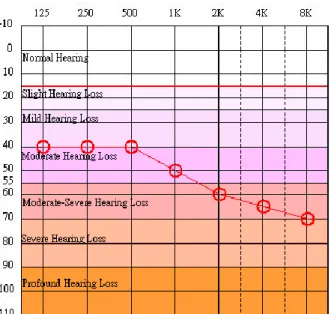
We recognized the sound by noting which frequencies contain the most energy. Hearing-impaired people have trouble understanding speech because essential parts of some phonemes are not audible. The hearing loss causes some frequencies components to be inaudible. Figure 2-2 is the audiogram of typical hearing-impaired person. The hearing-impaired person can’t hear clearly the sounds of the frequencies which are above 1000 Hz. For approximately 90% of hearing-impaired adults and for 75% of hearing-impaired children, the degree of impairment worsens from 500Hz to 4000Hz. Furthermore, the sound energy is dominated by low-frequency component.

Figure 2-2 Audiogram of typical hearing loss

In order to overcome these difficulties, a hearing aid needs to compensate the frequency-dependent audibility loss by amplifying the signal with various gains on each frequency. A filter bank is needed to decompose the signal into different frequency bands. Then the hearing aid has the capability to provide different amount of gain in different frequency regions.

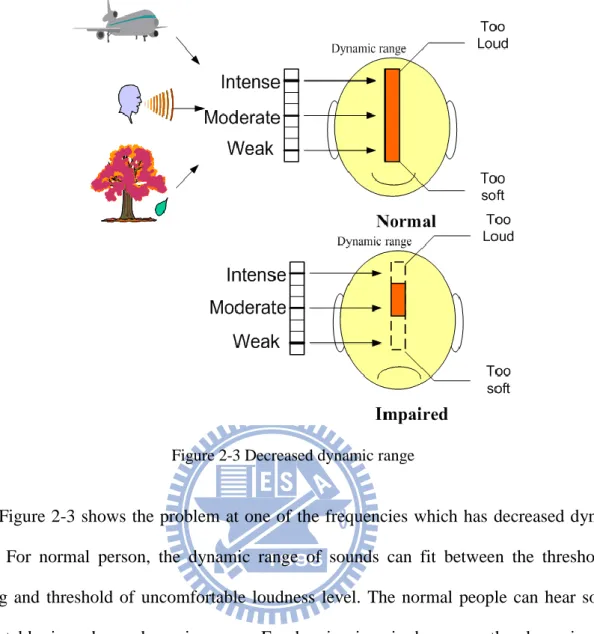
 Decreased dynamic range

Dynamic range is a term used frequently in numerous fields to describe the ratio between the smallest and largest possible values of a changeable quantity. The human ear has a dynamic range of about 130 dB between the threshold of just hearing and threshold of uncomfortable loudness level. In the above argument, soft sounds can be made audible by amplifying the sounds. Unfortunately, it is not appropriate to amplify everything for the same amount of gain. Because the dynamic range of a hearing-impaired ear is less than the dynamic range of the normal ear.

Figure 2-3 Decreased dynamic range

Figure 2-3 shows the problem at one of the frequencies which has decreased dynamic range. For normal person, the dynamic range of sounds can fit between the threshold of hearing and threshold of uncomfortable loudness level. The normal people can hear sounds comfortably in a large dynamic range. For hearing-impaired person, the dynamic range reduces. The weak sounds below the threshold of hearing and the intense sound exceed threshold of uncomfortable loudness level. They can’t hear weak to moderate sounds. If we only amplify the sound to make the weak sounds audible, the moderate to intense sound may exceed the uncomfortable loudness level and it is unacceptable for hearing-impaired people. For overcoming this difficult, hearing aids need to compress the input sounds. The hearing aid must provide more gains for soft sounds than intense sounds. The function reducing dynamic range of sounds is called dynamic range compression.

 SNR loss

less than a normal-hearing person in the same environment, even the hearing-impaired person is wearing hearing aid. In the other way, the hearing-impaired person needs a better signal-to-noise ratio (SNR) than does a normal-hearing person. Loss of clarity results in a loss of ability to understand speech, especially in noise. The noise reduction of the hearing aid can improve the signal-to-noise ratio and thus, improve speech intelligibility in the noisy listening environment.

 Frequency resolution loss

Another difficulty faced by people with sensorineural hearing loss is separating sounds of different frequencies. Different frequencies are represented most strongly at different place within the cochlea. When the cochlea gets damaged, it decreases the ability of the sensitivity to frequencies. If these frequencies are close enough, the cochlea will have a single broad region of activity rather than separate regions. The normal-hearing cochlea would separate the two broad regions. The impaired cochlea just recognizes a single broad region. For compensating the hearing loss, the speech enhancement function of the hearing aid improves some perceptual aspects of speech for the human listener.

2.2 Hearing aids & auditory compensation

2.2.1 Functions of advanced digital hearing aids

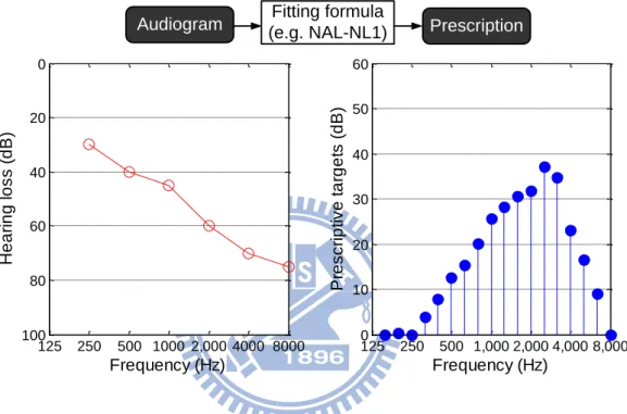
Hearing aids are hearing instruments that are designed to compensate the hearing loss and improve the speech intelligibility for hearing impaired people. As described in the Figure 2-4, a person’s hearing loss can be represented by an audiogram. The hearing thresholds in the audiogram describe the softest sounds that one can hear at the frequency. Then the prescriptive gains can be calculated from fitting formula to compensate the hearing loss and

maximize the speech intelligibility with respect to each audiogram. The most well-known fitting formula NAL-NL1 [2] calculates the amplification targets on 1/3-octave frequencies from 125 Hz to 8000 Hz defined in the ANSI S1.11 standard [3]. The main task of hearing aid is to selectively amplify the sounds such that processed sounds have a good match to one’s prescription.

Audiogram _{(e.g. NAL-NL1)}Fitting formula Prescription

125 250 500 1000 2,000 4000 8000 0 20 40 60 80 100 Frequency (Hz) H e a ri n g l o s s ( d B ) 125 250 500 1,000 2,000 4,000 8,000 0 10 20 30 40 50 60 Frequency (Hz) P re s c ri p ti v e t a rg e ts ( d B )

Figure 2-4 Audiogram & prescription

The block diagram of an advanced digital hearing aid is illustrated in Figure 2-5, which comprises four function blocks, i.e. the auditory compensation, echo cancellation, noise reduction and the speech enhancement. We focus on the auditory compensation algorithm which makes up for the perceptual distortion such as the raised hearing thresholds and the squeezed hearing dynamic ranges.

Band 1 Band 2 Band n … Gain 1 Gain 2 Gain n

Filter bank Compressor

Channel 1 Channel 2 Channel n + Echo concellation Noise reduction Speech enhancement Auditory compensation A/D D/A … …

Figure 2-5 Function of an advanced digital hearing aid

The auditory compensation system mainly contains two modules: a filter bank and a compressor. Filter bank decomposes the input signal into different frequency component and then the prescribed gains can be applied to each component to match the prescriptive targets. And the task of compressor is to dynamically reduce the gains to match the prescriptive targets at higher input level.

2.2.2 Delay requirement of hearing aids

An important concern in designing hearing aid is the overall delay. This time delay can cause disturbing effects to occur. For people who wear hearing aids, sounds are transmitted into the ear canal via two different paths. In the first path, signal transmits directly into ear canal with minimum delay via bone conduction. In the other path, the processed and delayed signal delivers to ear canal through hearing aids. These two paths have different time delays before perceived by the hearing aid user.

It is know that when the delay is about 10 milliseconds, the direct sound and the processed sound interact with each other and cause severe degradation to sound quality, known as comb filter effect. And when the delay becomes longer, the hearing impaired may notice an echo effect. And when even longer (more than 40 ms), the auditory information may

out of synchronization with the visual information and disturb lip reading. Besides, the effects of hearing aid delay are dependent on the severity of the hearing loss. As the hearing threshold worsens, the individual is able to hear less of the direct sound transmission and the delay is not as noticeable. The question is how much delay is acceptable for the majority of patients?

The delay introduced by the hearing aid has become more of an issue in the past 10 years. A summary of six recent papers related to the effects of delay in hearing aids is attached as follows. [3] ~ [8]

Table 2-1 Researches on the delay in hearing aids

Noticeable overall delay (ms) Objectionable overall delay (ms) Objectionable across-frequency delay (ms) Moore, 1999 [3] NA 20 NA Thornton, 2000 [4] 4 14 NA Moore, 2002 [5] NA 15 NA Moore, 2003 [6] NA NA 9 Kates, 2004 [7] 5 ~ 25 NA NA Moore, 2005 [8] NA 15 NA

Over the past 10 years, Stone and Moore have done many researches about tolerable hearing aid delay. In general, their findings suggest that disturbance increases monotonically with increasing delay, with delay times as low as 15 to 20 ms rated as disturbing for those with mild-to-moderate hearing losses. Another group of researchers working with actual commercial hearing aids found that delays larger than 10 ms may be objectionable to hearing aid user.

In summary, delays as short as 4 milliseconds that are constant across frequency are detectible for normal hearing people and 5 to 25 milliseconds are detectible for hearing impaired people depend on hearing loss. The overall delays in the range of 14 to 20 milliseconds can be judged as disturbing or objectionable.

2.3 Considerations for filter bank

 Matching prescription capability

As described in Section 2.2.1, the main task of hearing aid is to selectively compensate the hearing loss according to prescriptions such that make the sound audible and recognizable for hearing-impaired people. The auditory compensation system, especially the filter bank, has a great influence on the matching capability of a hearing aid, because the hearing aid is only able to adjust the gain on each sub-band signals. So, a filter bank with suitable spacing will be more flexible to adjust the magnitude response and have a better matching capability.

In general, a sound change of 3dB SPL is just noticeable for human ear. [10] To compensate the hearing loss properly, we can derive a necessary requirement that the maximum matching error of hearing aid’s frequency response to the prescriptive targets should keep smaller than 3dB.

 Digital signal processing delay (group delay)

As described in Section 2.2.2, the group delay is a crucial issue in hearing aids. The superposition of processed signal and the bypass signal may provoke strong comb filter effects for long signal processing group delay and degrade the sound quality.

Filter bank usually contributes the most group delay in the data path. But somehow it is the price that needs to pay to have a higher frequency resolution in the filter bank. And this can not be shortening according to the acoustic uncertainty principle. [11] It says that if we want to have a good resolution in frequency domain, more input samples need to be referenced in time domain and so introduce more group delays. That is, the narrower the channels are, the larger the group delay will have.

contribute from 2 to almost 5 ms group delay [12], we can derive the group delay specification for filter bank. The group delay of filter bank should not greater than 10ms.

 Signal processing complexity & power consumption

Due to the limited battery size in hearing aids, power consumption plays an important role. Algorithmic complexity is directly related to the power consumption so we must try our best to minimize the computation complexity. Filter bank usually contributes the most computational load. Therefore, signal processing algorithms have to be realized as efficient as possible.

2.4 Related works

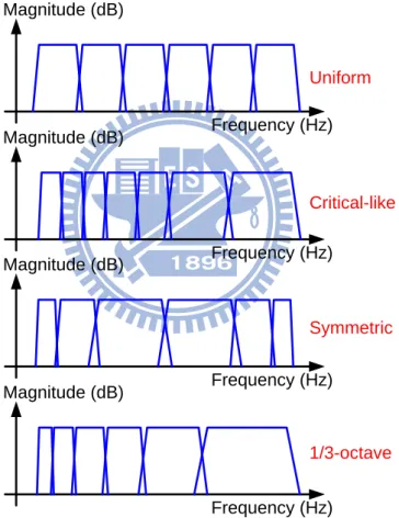
The auditory compensation, especially the filter bank, is an important function in hearing aids because it makes the sound audible for the hearing-impaired people. Famous prescriptive formula like NAL-NL1 or HSE give the amplification targets on 1/3-octave frequencies from 125Hz to 8000Hz. The filter bank should be designed to well match the prescriptions, so that the hearing loss can be compensated accurately and maximize the speech intelligibility. Furthermore, the overall signal processing delay and the power consumption is a critical issue for hearing aids as well as for the filter bank design. To the best of our knowledge, designing the filter bank for the digital hearing aids in the literature can be classified into two categories: uniform filter banks [13]~ [16] and non-uniform filter banks [17] ~ [20].

The uniform filter bank means that the bands are equally divided the frequencies from 0 to . A 16-band discrete Fourier transform (DFT) filter bank is designed in [13], while an 8-band filter bank with equal-spaced finite-impulse response (FIR) filters is implemented in [14]. [15] and [16] exploit the interpolation finite-impulse response (IFIR) techniques to realize a 7-band and a 8-band uniform filter bank respectively. The drawback of uniform filter

banks is that they do not match the non-uniform frequency characteristics in human auditory system. As a result, the uniform filter bank may face difficulties at matching the prescriptions for various types of hearing loss. Consequently, the using of non-uniform filter banks is more suitable.

As depicted in Figure 2-6, the common-used non-uniform filter banks can go a step further to classify into critical-band [17], symmetric-band [18][19], and 1/3-octave-band [20] filter banks. Frequency (Hz) Magnitude (dB) Frequency (Hz) Magnitude (dB) Frequency (Hz) Magnitude (dB) Frequency (Hz) Magnitude (dB) Uniform Critical-like Symmetric 1/3-octave

Figure 2-6 Different types of filter banks

In order to provide the frequency characteristics similar to that of the human auditory system, a critical-band filter bank is designed in [17]. The critical bands are divided according to psychoacoustics and have good match to human perception. However, the irregular property of the critical bands makes the implementation difficult. The design in [17], for

example, implements 16-band critical-like filter bank with rather high-order (110-tap) FIR filters, which has significant computation complexity. On the other hand, Lian and Wei proposed an 8-band and 16-band symmetric filter bank [18][19]. The symmetric filter bank is symmetric at /2 and has higher frequency resolution at both high and low frequencies. With the IFIR and frequency-response masking (FRM) techniques, the computational complexity is largely reduced. However, these symmetric banks have relatively small number of bands at middle frequencies and may not have sufficient resolutions for hearing loss compensation.

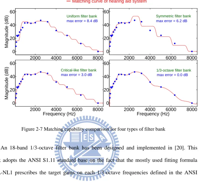
The preliminary results of matching capability for four types of filter bank are reported in Figure 2-7. Each type of filter bank is normalized to have 18 bands and designed at the sampling rate of 24 KHz. Then we evaluate the maximum matching error between the hearing aid’s frequency response and the 18 amplification targets prescribed by NAL-NL1. The uniform filter bank has equal-space bands from 0 to π. It has a lower frequency resolution in low frequencies so the matching error is large there. The maximum matching error is up to 8.4dB. The symmetric filter bank has a lower frequency resolution at middle frequencies. So, it has maximum matching error of 6.2dB at middle frequencies. The critical-like filter bank has a good match to the human hearing characteristics and the spacing is close to 1/3-octave filter bank at the middle and high frequencies. The bands are equally spaced at low frequencies, so it will have a larger error there. The maximum matching error is 3dB. Finally, by the use of 1/3-octave filter bank the hearing aid response can perfectly match the prescribed targets because the prescription formula calculates the prescriptions on 1/3-octave frequencies.

2000 4000 6000 8000 0 20 40 60 Frequency (Hz) Magnitud e (dB) 2000 4000 6000 8000 0 20 40 60 Frequency (Hz) Magnitud e (dB) 2000 4000 6000 8000 0 20 40 60 Frequency (Hz) Magnitud e (dB) 2000 4000 6000 8000 0 20 40 60 Frequency (Hz) Magnitud e (dB)

● 18 prescriptive targets from NAL-NL1 Matching curve of hearing aid system

Uniform filter bank Symmetric filter bank

Critical-like filter bank 1/3-octave filter bank

max error = 8.4 dB max error = 6.2 dB

max error = 3.0 dB max error = 0.0 dB

Figure 2-7 Matching capability comparison for four types of filter bank

An 18-band 1/3-octave filter bank has been designed and implemented in [20]. This work adopts the ANSI S1.11 standard base on the fact that the mostly used fitting formula NAL-NL1 prescribes the target gains on each 1/3-octave frequencies defined in the ANSI S1.11 standard. As a result, the hearing aid’s magnitude response can have the best capability to match any type of prescriptions by the use of ANSI S1.11 1/3-octave filter bank. The work also makes use of the multistage IFIR and multi-rate techniques to largely reduce the computational complexity (in terms of number of the multiplications per input sample). The complexity-effective architecture saves about 96% of multiplications comparing that with a straightforward FIR filter bank. However, the price this work pay is the long group delay which is up to 78ms and will largely limit the usage of this design. We observe that the unacceptable long group delay is due to the very sharp transition in lower frequency part of ANSI S1.11 1/3-octave bands. Even using the straightforward FIR or IIR to implement the filter bank, there still have group delay up to 27 ms and this can not be shortening further.

3 L

OW

-D

ELAY

F

ILTER

B

ANK

D

ESIGN

In this chapter, we propose a design method of 18-band 1/3-octave filter bank. The input sampling rate is 24 KHz to cover the whole frequency range that have prescribed amplification targets from NAL-NL1 fitting formula. Firstly, a quasi-ANSI S1.11 1/3-octave specification is developed to reduce the group delay. Secondly, we present a systematic design flow to design and optimize the FIR filter coefficients such that filter use minimized orders to meet the specification. Thirdly, a matching-error optimization method is proposed. Finally, the filter bank exploration results and verifications on various types of hearing loss will be demonstrated.

3.1 Quasi-ANSI S1.11 1/3-octave specification

The ANSI S1.11 standard is a specification for octave-band and fractional-octave-band analog and digital filters. This standard provides performance requirements for analog, sampled-data, and digital implementations of band-pass filters that comprise a filter set or spectrum analyzer for acoustical measurements. The extent of the pass-band region of a filter's relative attenuation characteristic is a constant percentage of the mid-band frequency for all filters.

ANSI S1.11 1/3-octave specification defines 43 bands in the 0 ~ 20 KHz frequency range. Each band is specified by its mid-band frequency fmand the bandwidth f . The mid-band frequency of nth band is defined as

r n

m n f

f ( )2( 30)/3  (3-1)

where f_r is the reference frequency and set to 1 KHz. For example, the mid-band frequency of the 22nd 1/3-octave band fm(22) is 160 Hz and the mid-band frequency of 39th band fm(39) is

8 KHz. We donate the lower and upper band-edge as f1 and f2 where

) 6 1 ( 1( ) ( ) 2    f n n f _m , and ) 6 1 ( 2

(

n

)



f

(

n

)



2

f

_m (3-2)

Then the bandwidth is defined between two band-edge frequencies

).

(

)

(

)

(

n

f

₂

n

f

₁

n

f







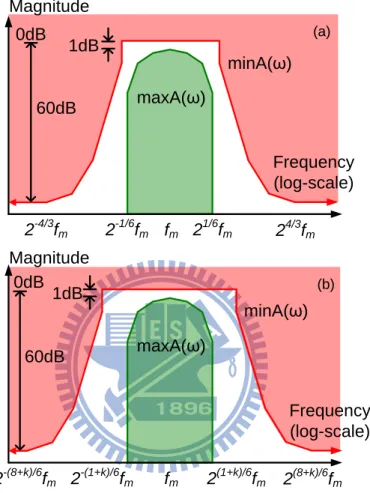
(3-3)

Magnitude 0dB 60dB Frequency (log-scale) fm 2 1/6 fm 2-1/6fm 2-4/3fm 24/3fm minA(ω) maxA(ω) 1dB (a)

Figure 3-1 Magnitude response limitation in ANSI S1.11 1/3-octave standard

Furthermore, Figure 3-1 (a) illustrates the magnitude specification for the nth 1/3-octave band, where maxA(ω) and minA(ω) describe the detail limits on the maximum and minimum attenuation of nth filter respectively. As shown in Figure 3-1, the pass-band ripple is allowed to be less than or equal to 1 dB, while the filter should have at least 60dB attenuation at frequencies smaller than fm

3 / 4

2 and at frequencies greater than24/3 f_m.

Based on the fact that the ANSI S1.11 1/3-octave filter bank is exponentially spaced in frequency domain, the frequency resolution will become two times higher every three bands. Bands are very narrow in low frequencies so we must use up to thousands of orders to design filter coefficients to meet the ANSI S1.11 1/3-octave standard. The group delay is a useful measure of time distortion, and is calculated by differentiating the phase response versus frequency. In other words, group delay is a measure of the slope of the filter’s phase response. A simpler way to calculate the group delay of linear phase FIR filter is that the group delay is equal to half of orders. The group delay in seconds can be calculate by equation (3-4)

rate sampling * 2 order delay group  _(3-4)

Parks-McClellan algorithm. But it still require 1488 orders in the lowest frequency band to meet the ANSI S1.11 1/3-octave filter bank standard. The sampling rate in [20] is 24 KHz. So we can calculate the group delay which is up 31ms, and is much larger then 10 ms. This fact also largely limits the applications of ANSI S1.11 1/3-octave filter bank in digital hearing aids. But ANSI S1.11 is still a good reference 1/3-octave filter bank specification because well-known hearing aid prescription formula NAL-NL1 also prescribes the amplification targets on each 1/3-octave frequencies defined in the ANSI S1.11 standard. As a result, we must slightly simplify the ANSI S1.11 1/3-octave filter bank specification at which the band’s group delay is larger then 10ms.

Remember that a useful formula derived experimentally by Kaiser [21] can be used to estimate the order of filter designed by Parks-McClellan algorithm.

 

W order p s     324 . 2 13 log 10 10   (3-5)

where δp andδs are the pass-band ripple and stop-band attenuation respectively and the W is the transition bandwidth. From equation (3-4) and (3-5) we can derive that the group delay of Parks-McClellan filter is linear proportionally to the transition bandwidth. The pass-band ripple and stop-band attenuation seem to be less sensitive to order by comparison.

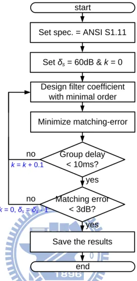
We propose a quasi-ANSI S1.11 1/3-octave filter design flow, which is outlined in Figure 3-2. The quasi-ANSI S1.11 1/3-octave filter has wider transition bandwidth then origin filter at low frequencies such that the group delay requirement is satisfied.

Minimize matching-error Design filter coefficient

with minimal order

no start Set δs = 60dB & k = 0 end Group delay < 10ms? yes

Set spec. = ANSI S1.11

Matching error < 3dB?

yes Save the results

k = k + 0.1

no

k = 0, δs = δs - 1

Figure 3-2 Quasi-ANSI S1.11 1/3-octave filter bank design flow

The development of quasi-ANSI S1.11 specification is conducted as follows. As depicted in Figure 3-3 (b), the magnitude response specification of maxA(ω) is kept unchanged. Then we stretch the minA(ω) specification by a factor k for the bands whose group delay are larger than 10 ms. The constraint on transition region will be released but the stop-band attenuation is still constrained to have more than 60dB and the pass-band ripple is still constrained to be less than 1dB. So, the limitation on the pass-band is without any degradation. The thing we do is to stretch the transition bandwidth specification such that the filter’s transition slope is flatter and reduce the group delay to below 10ms.

Then an exploration method will be described in Section 3.2. We propose an algorithm to explore the feasible solutions such that the filter meets the specification and the filter order is

minimized. A matching error optimization method is developed and described in Section 3.3. By finding the optimal insertion gains of each band, we can minimize the maximum matching error between the hearing aid response and the prescriptions.

0dB 60dB 1dB Frequency (log-scale) fm 2(8+k)/6fm Magnitude 0dB 60dB Frequency (log-scale) fm 2 1/6 fm 2-1/6fm 2-4/3fm 24/3fm minA(ω) maxA(ω) minA(ω) maxA(ω) 2(1+k)/6fm 2-(1+k)/6fm 2-(8+k)/6fm Magnitude 1dB (a) (b)

Figure 3-3 (a) Magnitude response limitation in ANSI S1.11 1/3-octave standard (b) Quasi-ANSI S1.11 1/3-octave specification

3.2 Filter coefficient design

To reduce the group delay as well as the computational complexity in filter, the orders of each filter should be determined as small as possible. We apply the widely-used Parks-McClellan algorithm to design the coefficients of each filter. Parks-McClellan algorithm is an optimum equiripple FIR design method [22]. The design parameters δp, δs, fs1,

ripple and stop-band attenuation respectively. fs1 and fs2 are stop-band bandage frequencies. fp1

and fp2 are pass-band bandage frequencies.

Magnitude 0dB Frequency δp δs fs1 fp1 fp2 fs2 TW1 TW2

Figure 3-4 Parameters for designing band-pass filter

Nevertheless, it is not straightforward to find the lowest-order filter such that the filter response satisfies the specification. So, we propose a filter coefficient design flow to design the filter as shown in Figure 3-5.

Explore feasible fs1 & fs2

Feasible fs1 & fs2 found? Estimate TW1 & TW2 no start TW1 x= 0.95 TW2 x= 0.95 Set δp = 1dB, δs = 60dB end yes Save TW1, TW2, fs1 & fs2

Figure 3-5 Filter coefficient design flow

According to the specification we set δp = 1dB and δs = 60dB. Then in order to reduce

by TW1 = fp1 – fs1 and TW2 = fs2 – fp2. The estimation of TW1 and TW2 can be conducted as

follows. We decompose the band-pass specification into low-pass and high-pass specification. Then design the low-pass filter (high-pass filter) that has maximum TW1 (TW2) and satisfies

the low-pass (high-pass) specification. Note that the maximized transition width leads to the minimized filter order. After we get the estimated transition width, we evaluate their feasibility. That is, we explore the possible values of fs1 and fs2 respectively to verify that

whether there exists a band-pass filter meets the specification. If the transition width TW1 and

TW2 are not feasible, it will be decreased by 5% each time alternately until the band-pass filter

meet the specification.

3.3 Minimize the matching-error

In hearing aid system, gain changes dynamically to satisfy different hearing loss people. ANSI S1.11 filter bank use the sharp transition to prevent the alias between neighbor bands. When fitting the hearing aid to match the prescriptions, an intuitive configuring method is to choose the prescribed gains as insertion gain of each sub-band. But the filter bank is not ideal, there are aliasing between bands. The insertion gain on one band will affect the others more or less depends on the amount of attenuation on the other bands. Because the quasi-ANSI S1.11 filter bank have flatter transition bandwidth in low frequencies, the aliasing is heavier between two neighbor bands, the insertion gains may affect neighbor frequencies. It will become more difficult to configure the hearing aid matching the prescriptive gains.

There have better choices for the insertion gains. We develop a configuration generator which can generate the configurations like insertion gains such that the hearing aid’s overall response can best match the prescriptions. The aliasing between bands are taken into consideration and compensated properly. By choosing the suitable insertion gains, the matching error can be minimized.

Firstly, we formula the matching error of mth prescribed gain as equation (3-6) | | log 20 18 1 ,       _ 



 n n m n m m P A G E (3-6)

where the amplitude of the mth prescribed gain is represented by Pm where m = 1, 2, 3, …, 18.

Similarly define the amplitude response of filter bank as An,m where represent the amplitude of

nth band at the frequency of mth prescribed gain. Let Gn denotes the amplitude of nth

insertion gain. Then



 18 1 , n n m n G

A represent the amplitude at the frequency of mth prescribed gains. So, we can derive the mth matching error Em to the mth prescribed gain.

Secondly, by using the minimization function called fmincon in MATLAB, we can find the optimal insertion gains Gn such that the maximum matching error of Em is minimal. The

syntax of fmincon is described in equation (3-7)

[G, error] = fmincon(objfun, xs, LB, UB) (3-7)

where objfun is the objective function and equal to max(Em) and Em is the matching error of

mth prescribed gain derived in equation (3-6). The initial condition value of insertion gains can be assigned by setting the xs. We set the initial value of insertion gains as prescribed gains. The LB and UB represent the lower and upper bound of insertion gains. Finally, the optimized insertion gains for each sub-band can be found and save to G. The error is save the maximum error to all prescribed gains.

3.4 Result & verifications

We evaluate the group delay and the maximum matching error with respect to different stretch factor k as reported in Table 3-1. With the increasing stretch factor k, the transition

bandwidth increase gradually and the group delay decreases from 27.3 ms to 9.4 ms. Notice that when the stretch factor goes from 1.2 to 1.4, the group delay is unchanged. This is because when the stretch factor is larger then 1.2, the stop-band frequency of the lowest-frequency band intersects the zero point. We only can stretch the transition bandwidth when the stop-band frequency is a positive value. Besides, the maximum matching error of prescribed targets increases from 0.8 dB to 7.1 dB. But after applying the matching-error optimization method, matching error only increase from 0dB to 2dB. Note that a feasible solution is found for stretch factor k larger than 0.8. The filter bank satisfy the group delay (smaller then 10 ms) and maximum error (smaller then 3dB) constraint.

Table 3-1 Group delay & matching error with respect to k

original with error reduction 0.0 27.3 0.8 0.0 0.2 21.6 1.1 0.0 0.4 17.0 1.5 0.8 0.6 13.4 2.4 1.4 0.8 10.0 3.3 1.5 1.0 9.8 4.2 1.5 1.2 9.4 5.7 1.9 1.4 9.4 7.1 2.0 Group delay (ms) Stretch factor k Matching error (dB)

The magnitude response of the quasi-ANSI S1.11 1/3-octave filter bank is depicted in Figure 3-6 and Figure 3-7. The bands in lower frequencies have a wider transition bandwidth to reduce the group delay. Besides, only the nine lowest-frequency bands have been modified, the other bands which are located at the frequencies larger then 1000Hz still satisfy the ANSI S1.11 1/3-octave standard.

2000 4000 6000 8000 10000 12000 -60 -40 -20 0 Frequency (Hz) Magnitud e (dB)

Figure 3-6 Magnitude response of quasi-ANSI S1.11 1/3-octave filter bank

500 1000 1500 2000 -60 -40 -20 0 Frequency (Hz) Magnitud e (dB) 500 1000 1500 2000 -60 -40 -20 0 Frequency (Hz) Magnitud e (dB)

(a)

(b)

Figure 3-7 Magnitude response comparison between (a) ANSI S1.11 1/3-octave filter bank (b) quasi-ANSI S1.11 1/3-octave filter bank

We use the quasi-ANSI S1.11 1/3-octave filter bank to match the prescriptions from NAL-NL1 of three different type of hearing loss as shown in Figure 3-8 ~ Figure 3-10. Firstly, the audiogram in Figure 3-8 is the most common type of hearing loss called presbycusis type

which is the hearing loss due to aging. The hearing loss will increase with the frequency. The maximum matching error of the 18 prescribed amplification target is 0.4dB. Secondly, the hearing loss in Figure 3-9 increases with the frequency decreases which is contrary to presbycusis type. Moreover, the hearing loss in Figure 3-10 is a severe hearing loss and is almost flat across all the frequencies. Because the difference of the adjacent prescribed gains is larger then the two cases before, this case is more difficult to match. The matching error is 1.5dB in this case and is still small then 3dB.

250 500 1000 2000 4000 8000 0 10 20 30 40 50 Frequency (Hz) M a g n itu d e ( d B ) matching curve prescribed targets 125 250 500 1000 2,000 4000 8000 0 20 40 60 80 100 120 Frequency (Hz) H e a ri n g l o s s ( d B ) 125 250 500 1,000 2,000 4,000 8,000 0 10 20 30 40 50 60 70 80 Frequency (Hz) P re s c ri p ti v e t a rg e ts ( d B ) Maximum matching error = 0.4dB

Figure 3-8 Matching result for hearing loss due to aging

250 500 1000 2000 4000 8000 0 10 20 30 40 50 Frequency (Hz) M a g n itu d e ( d B ) matching curve prescribed targets 125 250 500 1000 2,000 4000 8000 0 20 40 60 80 100 120 Frequency (Hz) H e a ri n g l o s s ( d B ) 125 250 500 1,000 2,000 4,000 8,000 0 10 20 30 40 50 60 70 80 Frequency (Hz) P re s c ri p ti v e t a rg e ts ( d B ) Maximum matching error = 0.4dB

250 500 1000 2000 4000 8000 0 10 20 30 40 50 Frequency (Hz) M a g n itu d e ( d B ) matching curve prescribed targets 125 250 500 1000 2,000 4000 8000 0 20 40 60 80 100 120 Frequency (Hz) H e a ri n g l o s s ( d B ) 125 250 500 1,000 2,000 4,000 8,000 0 10 20 30 40 50 60 70 80 Frequency (Hz) P re s c ri p ti v e t a rg e ts ( d B ) Maximum matching error = 1.5dB

Figure 3-10 Matching result for severe flat hearing loss

In order to evaluate the matching capability of the proposed filter bank, we are going to examine it using various hearing loss audiograms. The results are illustrated in Figure 3-11 ~ Figure 3-16. These audiograms are downloaded from the Independent Hearing Aid Information which is a public service by Hearing Alliance of America. [23] These audiograms are also adopted in [18] to verify the matching capability. But the work in [18] is trying to match the audiograms itself not the prescriptions. We think that we can compensate the hearing loss more properly by matching the prescriptions to the hearing loss. If we fitting our hearing aid to match the audiograms, it may have the amplification exceed actually what hearing loss people need. Moreover, matching the audiograms is easier due to less amplification targets. Even through it is more difficult to match the prescriptions, the matching results show that the proposed filter bank can have a much smaller matching error compared to the filter bank design in [18].

In the following, the hearing loss levels are defined as described in Figure 2-2 and summarized as follows.

 Normal hearing: 0 ~ 19 dB

 Moderate hearing loss: 40 ~ 59 dB

 Severe hearing loss: 60 ~ 89 dB

 Profound hearing loss: 90 + dB

Figure 3-11 shows an audiogram with mild hearing loss around frequency 4 KHz. Such kind of hearing loss results probably from diseases or career injury. People can not hear most consonants and will have severe trouble in noisy environments. The maximum matching error is 0.2 dB, while that in [18] is about 8 dB after optimization. Therefore the maximum matching error is considerably reduced.

125 250 500 1000 2,000 4000 8000 0 20 40 60 80 100 120 Frequency (Hz) H e a ri n g l o s s ( d B ) 125 250 500 1,000 2,000 4,000 8,000 0 10 20 30 40 50 60 70 80 Frequency (Hz) P re s c ri p ti v e t a rg e ts ( d B ) 250 500 1000 2000 4000 8000 0 10 20 30 40 50 Frequency (Hz) M a g n itu d e ( d B ) matching curve prescribed targets Maximum matching error = 0.2dB

Figure 3-11 Matching result for mild hearing loss at 4 KHz

Figure 3-12 shows an audiogram with mild hearing loss in the whole frequencies. People with such kind of hearing loss have difficulties in hearing most vowels and consonants and will have more trouble in noisy conditions. The maximum matching error is 0.2 dB, whereas that in [18] is about 3.5 dB after gain optimization. The matching accuracy is higher than that in [18].

250 500 1000 2000 4000 8000 0 10 20 30 40 50 Frequency (Hz) M a g n itu d e ( d B ) matching curve prescribed targets 125 250 500 1000 2,000 4000 8000 0 20 40 60 80 100 120 Frequency (Hz) H e a ri n g l o s s ( d B ) 125 250 500 1,000 2,000 4,000 8,000 0 10 20 30 40 50 60 70 80 Frequency (Hz) P re s c ri p ti v e t a rg e ts ( d B ) Maximum matching error = 0.2dB

Figure 3-12 Matching result for mild hearing loss in whole frequencies

Figure 3-13 shows an audiogram with mild to moderate hearing loss at low frequencies and mild hearing loss at high frequencies. The primary effect will be a loss of overall loudness because most vowels cannot be heard. Very close distance conversations may be necessary. The maximum matching error is 0.1 dB, whereas that in [18] is about 2.5 dB after gain optimization. 125 250 500 1000 2,000 4000 8000 0 20 40 60 80 100 120 Frequency (Hz) H e a ri n g l o s s ( d B ) 125 250 500 1,000 2,000 4,000 8,000 0 10 20 30 40 50 60 70 80 Frequency (Hz) P re s c ri p ti v e t a rg e ts ( d B ) 250 500 1000 2000 4000 8000 0 10 20 30 40 50 Frequency (Hz) M a g n itu d e ( d B ) matching curve prescribed targets Maximum matching error = 0.1dB

Figure 3-13 Matching result for mild to moderate hearing loss in low frequencies

has moderate to profound hearing loss at middle to high frequencies. As the frequency becomes higher, the hearing impaired has higher hearing loss. The sensitivity at low frequencies is relatively good to get some vowel information and know that someone is talking. However, the loss of too many consonants will make one unable to distinguish one word from another. The maximum error is 0.3 dB, whereas that in [18] is about 8 dB after optimization. The matching error is significantly reduced.

125 250 500 1000 2,000 4000 8000 0 20 40 60 80 100 120 Frequency (Hz) H e a ri n g l o s s ( d B ) 125 250 500 1,000 2,000 4,000 8,000 0 10 20 30 40 50 60 70 80 Frequency (Hz) P re s c ri p ti v e t a rg e ts ( d B ) 250 500 1000 2000 4000 8000 0 10 20 30 40 50 Frequency (Hz) M a g n itu d e ( d B ) matching curve prescribed targets Maximum matching error = 0.3dB

Figure 3-14 Matching result for hearing loss due to aging

Figure 3-15 shows a type of hearing loss which is common seen in older workers in noisy industries and has severe hearing loss in middle to high frequencies. It is generally due to the effects of too much noise for too many years on the inner ear and related structures. Note that in the lower frequencies, the hearing sensitivity is good enough to give some vowel information. However, the high hearing loss in high frequency leads to miss so many consonants and may have a large problem distinguishing one word from another. The maximum error is 0.6 dB, whereas that in [18] is about 8 dB after optimization. The matching error is significantly reduced.

125 250 500 1000 2,000 4000 8000 0 20 40 60 80 100 120 Frequency (Hz) H e a ri n g l o s s ( d B ) 125 250 500 1,000 2,000 4,000 8,000 0 10 20 30 40 50 60 70 80 Frequency (Hz) P re s c ri p ti v e t a rg e ts ( d B ) 250 500 1000 2000 4000 8000 0 10 20 30 40 50 Frequency (Hz) M a g n itu d e ( d B ) matching curve prescribed targets Maximum matching error = 0.6dB

Figure 3-15 Matching result for hearing loss

Figure 3-16 shows an audiogram with severe to profound hearing loss at all frequencies, where almost all hearing thresholds are around 90 dB. Because the hearing loss is severe to profound, the prescribed gains are very large and change largely between two gains. It is difficult to match all of the amplification targets. The maximum error is 2.5 dB. It is well known that people are not sensitive to a matching error below 3 dB, so the matching result is satisfactory. 250 500 1000 2000 4000 8000 0 10 20 30 40 50 60 70 80 Frequency (Hz) M a g n itu d e ( d B ) matching curve prescribed targets 125 250 500 1000 2,000 4000 8000 0 20 40 60 80 100 120 Frequency (Hz) H e a ri n g l o s s ( d B ) 125 250 500 1,000 2,000 4,000 8,000 0 10 20 30 40 50 60 70 80 Frequency (Hz) P re s c ri p ti v e t a rg e ts ( d B ) Maximum matching error = 2.5dB

4 I

MPLEMENTATION

R

ESULTS

We exploit the natural property of 1/3-octave filter bank to design a complexity-effective architecture by the use of multirate & interpolated finite-impulse response (IFIR) techniques. We fold our filter bank into an architecture using only one filter to reduce the complexity. To avoid the computation conflicts or stalls, the scheduling method is also provided to minimize the required storage elements. Besides, we apply some low-power techniques to reduce the power consumption.

4.1 Complexity-effective architecture design

FIR digital filters are well known to have some desirable properties like stability and linear phase response. The main drawback of it is the large mount of arithmetic operations needed in implementation, especially for the filters with narrow transition bandwidth. In order to cope with the computational complexity of sharp narrowband FIR filters, the interpolated finite-impulse response (IFIR) filter technique is introduced [24].

Magnitude (dB) Frequency (Hz) H(z) G(z) G(zL) I(z) fs1 fp1 fp2 fs2 L(fp1 - fs1) 2π/L fs2 (fp1 - fs1)

…

…

…

…

G(zL) I(z) H(z) fs1 fp1 fp2 fs2

Figure 4-1 IFIR implementation of H(z) (frequency domain)

Suppose the band-pass filter H(z) with the specification [δp, δs, fs1, fs2, fp1, fp2] as

described in Figure 3-4. The basic IFIR structure can be composed of an image suppression filter I(z) and a model filter G(z) where L is the interpolation factor. IFIR filter is to implement the filter H(z) as a cascade of two FIR sections which are I(z) and G(zL) as described in Figure 4-1. G(zL) is produced from G(z). The impulse response of G(zL) is formed by interpolating the impulse response of G(z) by a factor L and padded with zero. Figure 4-2 illustrates the

relationship between G(z), G(zL), I(z) and H(z) in time domain for a interpolation factor of 2. From the view of hardware implementation, G(zL) is formed by using L storage elements to replace the original single storage element in G(z). Besides, I(z) is a image suppressor. In frequency domain analysis, G(zL) has a periodic frequency response at high frequencies called image terms with period 2π/L. The task of I(z) is to suppress the unwanted image terms of basic pass-band filter at higher frequencies. In time domain analysis, the meaning of the cascaded I(z) and G(zL) is that I(z) try to “fill in” the expected value of impulse response to G(zL) in stead of “filling in” zero which will generates high frequency image, as described in

Figure 4-2.

Amplitude

n

n

n

n

G(z)

G(z

2

)

I(z)

H(z)

G(zL) I(z) H(z)

Figure 4-2 IFIR implementation of H(z) (time domain)

terms of multiplications per sample) of G(z) will decrease and the complexity of I(z) will increase. There exists an optimal interpolation factor L such that the complexity of H(z) is minimized. We can evaluate this value through some analytical derivation as follows. Suppose the band-pass filter H(z) with the specification [δp, δs, fs1, fs2, fp1, fp2] as described in Figure 3-4.

Rely on the order estimation formula of Kaiser [21], we can estimate the order of optimal equaripple FIR filter which is designed by using Park-McClellan algorithm.

 





W D W N ps p,s 324 . 2 13 log 10 ₁₀      (4-1)

Besides, by exploiting the symmetry property of linear phase FIR filter, the number of multiplications per input sample can be approximate by N/2. Hence, the total number of multiplications per sample of H(z) can be expressed as (4-2)





                     _                   2 2 1 1 2 , 2 , 2 2 1 2 2 # p s s p s p s p I G f f L D f f L D N N Mult      (4-2)

where Ng is the order of G(z) and Ni is the order of I(z). The terms L



fp1 fs1



and 2 2 2 p s f f L       _

are the minimum transition bandwidth of G(z) and I(z) respectively. The

pass-band ripple is estimated to be roughly half of the desired ripple specification. Finally, we can evaluate the complexity for all possible integer values of L to obtain the optimal interpolation factor for each filter.

With carefully selecting the interpolation factor L and choosing the best method to implement each band’s filter, there will be an optimum IFIR filter design with minimum hardware complexity. The price paid for these reductions is only a slight increase in the

number of delay elements as compared with direct implementation.

For example, we use the IFIR technique described above to design the lowest frequency band. Let the band-pass filter specification is as follows.

         dB dB Hz f Hz f Hz f Hz f s p s s p p 60 1 300 10 168 149 2 1 2 1   (4-3)

A conventional linear-phase Parks-McClellan linear phase FIR filter design requires orders up to 368. It requires 189 multiplications per input sample and 368 storage elements to buffer the input sample. After using the IFIR filter implementation method, it only requires 33 multiplications per input sample and the required storage elements slightly increase to 388. The exploration of the computational complexity (in terms of multiplications per sample) with respect to different L is shown in Figure 4-3. With the increasing of the interpolation factor L the computational complexity of G(z) will largely decrease at the beginning and the complexity of I(z) will increase gradually. Finally, we can implement the filter with optimal IFIR filter structure. That is, when the interpolation factor is equal to 10, the filter will have minimum hardware complexity. The detail value for each interpolation factor is listed in Table 4-1.

2

4

6

8

10

12

14

16

0

20

40

60

80

100

Interpolation factor L

N

u

m

b

e

r

o

f

m

u

ltip

lica

tio

n

s

p

e

r

sa

m

p

le

H(z) G(z) I(z) Optimal factor = 10 H(z) G(z) I(z)

Figure 4-3 Explore the optimal L for IFIR filter implementation

Table 4-1 Computational complexity (multiplications per sample) with different L

L 2 3 4 5 6 7 8 # mult. of G(z) 90 59 44 36 30 25 22 # mult. of I(z) 1 4 5 7 8 10 11 # mult. of H(z) 91 63 49 43 38 35 33 order of H(z) 362 362 362 374 376 370 374 L 9 10 11 12 13 14 15 # mult. of G(z) 20 18 16 15 14 13 12 # mult. of I(z) 13 14 16 20 24 27 30 # mult. of H(z) 33 32 32 35 38 40 42 order of H(z) 386 388 384 396 412 418 420

In addition to the IFIR implementation method, we also exploit the multirate processing technique. Multirate means multiple data rates and it offers many advantages, such as reduced computational complexity for a given task, reduced transmission rate, and reduced storage

requirement. Broadly speaking, if the filter is band-limit and its stop-band frequency is lower then /M, we can down-sample the filter by a factor of M to reduce the data rate. The M is called decimation rate. Ones the data rate is reduced, the computational complexity (multiplications per sample) are reduced. The filter can process the input sample once upon every M sample. By the theory of multirate systems [24], a synthesis bank with up-sampler and interpolation filter is necessary. The task of interpolation filter is to suppress the image terms in higher frequencies after the signal is up-sampled. So, the price needs to pay is the cost of the interpolation filter in synthesis bank. The interpolation filter will contribute extra computational complexity. This is a trade-off between analysis bank and synthesis bank. When the decimation factor M increase, we have a lower data rate and can save more computational complexity in the analysis bank. But when the decimation factor M increase, we need an interpolation filter with narrower transition bandwidth and so have larger computational complexity in the synthesis bank.

Considering the architecture shown in Figure 4-4 (a), the cascaded IA(z) and G(zL) is the

IFIR implementation architecture described before. Then by the noble identity of the theory of multirate systems, we can derive the architecture in Figure 4-4 (b). Because the data rate is down-sampled by a factor M, the filter G(z) can process the sample once for every M sample. More over, G(z) only need to buffer one sample from IA(z) for every M sample. As a result,