國⽴臺灣⼤學理學院應⽤數學科學研究所 碩⼠論⽂
Institute of Applied Mathematical Sciences College of Science
National Taiwan University Master Thesis
利⽤⾼度平⾏之演算法整合多重隨機奇異值分解並應
⽤於巨量資料分析
Highly Scalable Parallelism of Integrated Randomized Singular Value Decomposition with Big Data Applications
楊慕 Mu Yang
指導教授:王偉仲 博⼠
Advisor: Weichung Wang, Ph. D.
中華民國 106 年 7 ⽉
July, 2017
誌謝
在此論⽂完成之際,必須要感謝在我研究路程上幫助我的所有⼈,
沒有你們的幫助,我無法有現在的成果。
在研究過程中,給予我最多幫助的是我的指導教授 王偉仲博⼠,
從認識他以來,他不遺餘⼒地指導我的學習,帶給我許多收穫。他的 辦公室⼤⾨始終對我敞開,每當我的研究或寫作有新的進展或是遇到 瓶頸時,總是不厭其煩的與我討論並給予全⾯性的回應。在王⽼師的 帶領下,我獲得許多機會參與各個學術會議及參訪,得以與各領域的 專家交流,對我的研究有相當程度的幫助。此外,也⾮常感謝中央研 究院統計科學研究所的陳素雲博⼠與陳定⽴博⼠,他們的研究在這個 領域上奠下基⽯,我能夠做出此研究並寫出論⽂,可說是站在巨⼈的 肩膀上。
我衷⼼感謝我的同學張⼤衛,他熱情的參與和投⼊,極⼤地協助了 我的研究⼯作,與他的討論啟發了我很多想法。在寫作上他也給了我 很多意⾒,⼤⼤改善了論⽂的品質。此外,還要感謝東京⼤學情報基 盤中⼼提供 Reedbush-U/H 超級電腦系統,以及周世恩學⾧提供臉書資 料庫,幫助我完成這份論⽂的數值測試。也感謝我研究室的同伴們,
不僅在研究上給予我許多幫助,也提供我最歡樂的研究環境,並在我 遇到瓶頸給予我精神上的⽀持。
最後,感謝我的家⼈這些年來給予我的⽀持與關懷,讓我得以求學
⽣涯中無後顧之憂,專⼼於學習與研究。謹以本⽂獻給我敬愛的家⼈
與所有關⼼我的⼈,並將這份成果呈獻給你們。
Acknowledgements
I’m glad to express my sincere gratitude to my thesis advisor Dr. We- ichung Wang of the Institute of Applied Mathematical Sciences at National Taiwan University for his support of my study and research. The door to Prof.
Wang’s office was always open whenever I ran into a trouble spot or had a question about my research or writing.
I also like to show my gratitude to Dr. Su-Yun Huang and Dr. Ting-Li Chen at the Institute of Statistical Science of Academia Sinica. Without their insight and expertise, the research could not have been successfully con- ducted.
My sincere thanks also go to my colleague Dawei Chang for his passionate participation and input that greatly assisted the research. The discussion with him inspires me a lot. He also gave me many comments that greatly improved the manuscript.
I would also like to thank the Information Technology Center at the Uni- versity of Tokyo for providing Reedbush-U/H supercomputer systems, and Mr. Shih-En Chou for providing the Facebook datasets. I am glad to thank my fellow labmates for the stimulating discussions, and for all the fun we have had.
Last but not the least, I would like to thank my family for supporting me spiritually throughout my life.
摘要
低秩近似在⼤數據分析中佔了重要的地位,整合奇異值分解(Inte- grated Singular Value Decomposition,iSVD)是⼀種⽤於計算⼤矩陣的 低秩近似奇異值分解的演算法。iSVD 集成了從多個隨機⼦空間抽樣
⽽獲得的不同的低秩奇異值分解,並達到更⾼的精準度和更好的穩定 性。雖然多個隨機抽樣與合併的過程需要更⾼的計算成本,但由於這 些操作可以平⾏化,iSVD 仍然可以節省計算時間。我們在多核⼼計 算集群上平⾏此演算法,並對計算⽅法及資料結構進⾏了修改,以增 加可擴展性並減少資料傳輸。透過平⾏化,iSVD 可以找到巨⼤矩陣 的近似奇異值分解,達到相對於矩陣尺⼨和機器數量接近線性的可擴 展性,並透過使⽤ GPU 在抽樣的步驟達到四倍的加速。我們⽤ C++
實作此演算法,並應⽤了幾種提⾼可維護性、可擴展性和可⽤性的技 術。我們在使⽤混合 CPU-GPU 的超級電腦系統上使⽤ iSVD 求解⼀些
⼤規模的應⽤問題。
關鍵詞:奇異值分解,平⾏演算法,分散式演算法,隨機演算法,
圖形處理器,⼤數據分析
Abstract
Low-rank approximation plays an important role in big data analysis. In- tegrated Singular Value Decomposition (iSVD) is an algorithm for computing low-rank approximate singular value decomposition of large size matrices.
The iSVD integrates different low-rank SVDs obtained by multiple random subspace sketches and achieve higher accuracy and better stability. While iSVD takes higher computational costs due to multiple random sketches and the integration process, these operations can be parallelized to save compu- tational time. We parallelize iSVD for multicore clusters, and modify the algorithms and data structures to increase the scalability and reduce commu- nication. With parallelization, iSVD can find the approximate SVD of ma- trices with huge size, and achieve near-linear scalability with respect to the matrix size and the number of machines, and gained further 4X faster tim- ing performance on sketching by using GPU. We implement the algorithms in C++, with several techniques for high maintainability, extensibility, and usability. The iSVD is applied on some huge size application using hybrid CPU-GPU supercomputer systems.
Keywords. Singular value decomposition, Parallel algorithms, Distributed algorithms, Randomized algorithms, Graphics processing units, Big data anal- ysis
Contents
⼝試委員會審定書 iii
誌謝 v
Acknowledgements vii
摘要 ix
Abstract xi
1 Introduction 1
2 Algorithms 5
2.1 Integrated Singular Value Decomposition . . . 5
2.2 Stage I: Sketching . . . 6
2.3 Stage II: Orthogonalization . . . 7
2.4 Stage III: Integration . . . 8
2.5 Stage IV: Postprocessing . . . 11
3 Improvements of Integration 15 3.1 Optimization Problem . . . 15
3.2 Improvements of Kolmogorov-Nagumo Integration . . . 17
3.3 Improvements of Wen-Yin Integration . . . 19
3.4 Integration Using the Gramian of𝕼 . . . 22
4 Parallelism 27
4.1 Naïve Parallelism . . . 27
4.2 Block-Row Parallelism for Integration . . . 28
4.3 Block-Row Parallelism for Gramian Integration . . . 32
4.4 Block-Row Parallelism for Sketching, Orthogonalization, and Postpro- cessing . . . 34
4.5 Block-Column Parallelism . . . 38
4.6 GPU Acceleration . . . 41
5 Comparison of Algorithms 43 6 Implementation 45 6.1 C++ Implementation . . . 45
6.1.1 Object Oriented Programming . . . 45
6.1.2 C++11 Standard . . . 46
6.1.3 Template Meta-Programming . . . 46
6.1.4 Curiously Recurring Template Pattern . . . 46
6.1.5 Data Storage and Linear Algebra Wrappers . . . 47
6.2 Parallelism . . . 47
6.2.1 MPI . . . 47
6.2.2 OpenMP . . . 47
6.2.3 GPU . . . 47
6.3 Tools . . . 48
6.3.1 CMake . . . 48
6.3.2 Google Test . . . 48
6.4 Package Structure . . . 49
7 Numerical Results 51 7.1 Comparison of Parallelisms . . . 51
7.2 Scalability of Integration Algorithms . . . 53
7.3 Implementation and Big Data Applications . . . 55
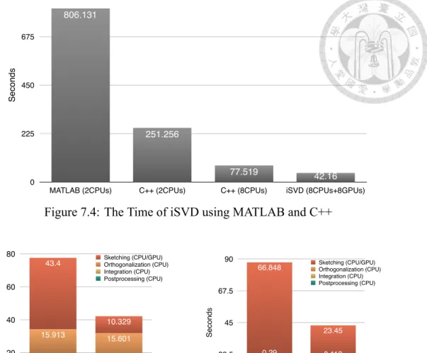
7.3.1 Comparison with MATLAB . . . 56
7.3.2 Facebook 100k . . . 56
7.3.3 1000 Genomes Project . . . 57
8 Conclusion 59 Bibliography 61 A Derivations 65 A.1 Derivation of Hierarchical Reduction Integration . . . 65
A.2 Derivation of Tall Skinny QR . . . 66
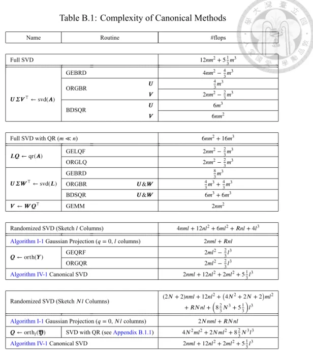
B Complexity 69 B.1 Canonical Methods . . . 70
B.1.1 𝖄 Orthogonalization . . . 71
B.2 Sequential Algorithms . . . 72
B.2.1 Stage I: Sketching . . . 72
B.2.2 Stage II: Orthogonalization . . . 72
B.2.3 Stage III: Integration . . . 73
B.2.4 Stage IV: Postprocessing . . . 76
B.3 Parallel Algorithms . . . 77
B.3.1 Stage I: Sketching (Parallelism) . . . 77
B.3.2 Stage II: Orthogonalization (Parallelism) . . . 78
B.3.3 Stage III: Integration (Parallelism) . . . 79
B.3.4 Stage IV: Postprocessing (Parallelism) . . . 84
List of Figures
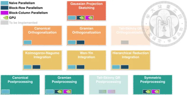
6.1 The Table of Implemented Algorithms . . . 48
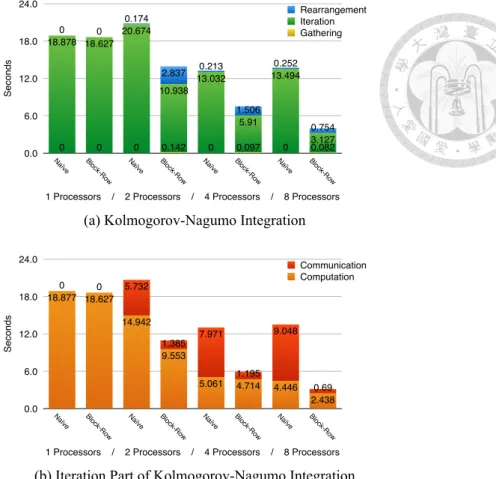
7.1 Comparison of Naïve and Block-Row Parallelism . . . 52
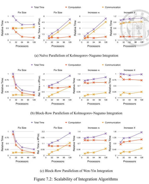
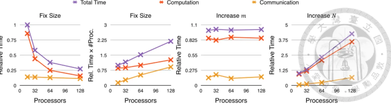
7.2 Scalability of Integration Algorithms . . . 53
7.4 The Time of iSVD using MATLAB and C++ . . . 56
7.5 The Time of iSVD using CPU and GPU . . . 56
List of Tables
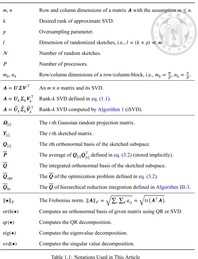
1.1 Notations Used in This Article . . . 3
3.1 Notations and Formulas Used in Optimization Integrations . . . 16
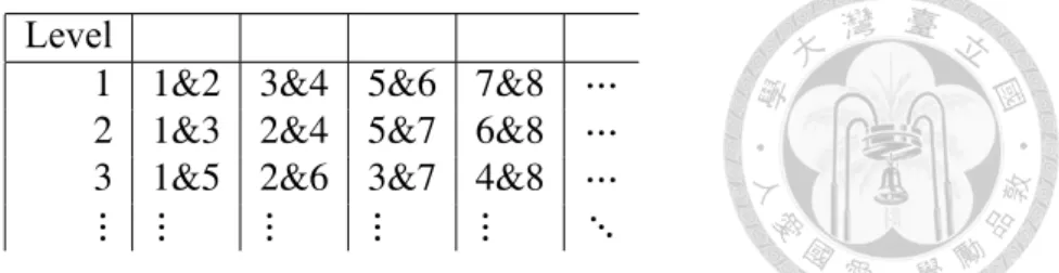
4.1 Communication Tree of Tall Skinny QR . . . 37
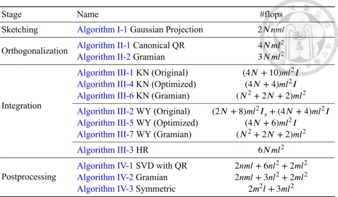
5.1 The Complexity of Sequential Algorithms . . . 44
5.2 The Complexity of Block-Row Algorithms . . . 44
5.3 The Complexity of Block-Column Algorithms . . . 44
B.1 Complexity of Canonical Methods . . . 70
B.2 Complexity of𝖄 Orthogonalization . . . 71
B.3 Complexity of Sketching . . . 72
B.4 Complexity of Orthogonalization . . . 72
B.5 Complexity of Integration . . . 73
B.8 Complexity of Postprocessing . . . 76
B.9 Complexity of Sketching (Naïve Parallelism) . . . 77
B.10 Complexity of Sketching (Block-Row Parallelism) . . . 77
B.11 Complexity of Sketching (Block-Column Parallelism) . . . 77
B.12 Complexity of Orthogonalization (Naïve Parallelism) . . . 78
B.13 Complexity of Orthogonalization (Block-Row Parallelism) . . . 78
B.14 Complexity of Integration (Naïve Parallelism) . . . 79
B.15 Complexity of Integration (Block-Row Parallelism) . . . 80
B.19 Complexity of Postprocessing (Block-Row Parallelism) . . . 84
B.21 Complexity of Postprocessing (Block-Column Parallelism) . . . 86
List of Algorithms
Main Algorithms
1 Integrated Singular Value Decomposition . . . 6
Sketching Algorithms I-1 Gaussian Projection Sketching . . . 7
I-2 Gaussian Projection Sketching (Block-Row Parallelism) . . . 35
I-3 Gaussian Projection Sketching (Block-Column Parallelism) . . . 39
Orthogonalization Algorithms II-1 Canonical Orthogonalization . . . 7
II-2 Gramian Orthogonalization . . . 7
II-3 Gramian Orthogonalization (Block-Row Parallelism) . . . 35
II-4 TSQR Orthogonalization (Block-Row Parallelism) . . . 37
Integration Algorithms III-1 Kolmogorov-Nagumo Integration . . . 9
III-2 Wen-Yin Integration . . . 10
III-3 Hierarchical Reduction Integration . . . 11
III-4 Kolmogorov-Nagumo Integration (Optimized) . . . 19
III-5 Wen-Yin Integration (Optimized) . . . 22
III-6 Kolmogorov-Nagumo Integration (Gramian) . . . 24
III-7 Wen-Yin Integration (Gramian) . . . 25
III-8 Kolmogorov-Nagumo Integration (Naïve Parallelism) . . . 28 III-9 Hierarchical Reduction Integration (Naïve Parallelism) . . . 28 III-10Kolmogorov-Nagumo Integration (Block-Row Parallelism) . . . 30 III-11Wen-Yin Integration (Block-Row Parallelism) . . . 31 III-12Hierarchical Reduction Integration (Block-Row Parallelism) . . . 32
Postprocessing Algorithms
IV-1 Canonical Postprocessing . . . 12 IV-2 Gramian Postprocessing . . . 12 IV-3 Symmetric Postprocessing . . . 13 IV-4 Gramian Postprocessing (Block-Row Parallelism) . . . 36 IV-5 Symmetric Postprocessing (Block-Row Parallelism) . . . 36 IV-6 TSQR Postprocessing (Block-Row Parallelism) . . . 38 IV-7 Gramian Postprocessing (Block-Column Parallelism) . . . 39 IV-8 TSQR Postprocessing (Block-Column Parallelism) . . . 40 IV-9 Symmetric Postprocessing (Block-Column Parallelism) . . . 41
Subroutines
S-1 Matrices Rearrangement (Block-Row Parallelism) . . . 33 S-2 Computing𝕭 = 𝕼⊤𝕼 (Block-Row Parallelism) . . . 33 S-3 Computing𝑩𝑐 = 𝕼⊤𝑸init (Block-Row Parallelism) . . . 33 S-4 Computing𝑸opt = 𝑸init𝑭 + 𝕼 ̃̃ 𝑬 (Block-Row Parallelism) . . . 33 S-5 Matrices Gathering (Block-Row Parallelism) . . . 34
Chapter 1 Introduction
Big data analysis is one of the important fields in nowadays. We often use low-rank ap- proximation for feature selection and dimension reduction. Singular value decomposition (SVD) is one of an essential tool for finding low-rank approximations. In this article, we consider the rank-𝑘 singular value decomposition
𝑨 = 𝑼 𝜮𝑽⊤ ≈ 𝑼𝑘𝜮𝑘𝑽𝑘⊤, (1.1)
where𝑼 𝜮𝑽⊤is the full SVD and𝑼𝑘𝜮𝑘𝑽𝑘⊤is the truncated rank-𝑘 SVD. However, tradi- tional algorithms may take about12𝑛𝑚2flops (assuming𝑚 < 𝑛) for computing the SVD of an𝑚 × 𝑛 matrix 𝑨, which lack scalability and leads to a computational problem when the matrix size is large. Randomized singular value decomposition (rSVD) [1,2] reduces the computational cost to4𝑛𝑚𝑘 flops. Furthermore, Chen et al. proposed an efficient algo- rithm, integrated singular value decomposition (iSVD) (Algorithm 1) [3], which integrates the results from multiple rSVDs and achieve higher accuracy.
In this article, we focus on the implementation and the application of iSVD on large- scale clusters. The development of supercomputer allows us to handle huge scale prob- lems. Multithread and multicore parallelization can speed up the computations. The com- putation is also benefited from GPU acceleration on hybrid CPU-GPU architecture. In these machine structures, data communication becomes an essential problem.
We modify the iSVD algorithms that reuse the matrices to reduce the computational
cost. For large-scale clusters, we propose new data structure for parallel algorithms to reduce data communication so that the communication cost is independent of the size of the problem. These algorithms are balanced and weak scalable. We compare the compu- tational and communication complexity of each algorithm, and recommend the suitable choice for different shapes of the input matrix. The iSVD is implemented in C++ with several techniques for high maintainability, extensibility, and usability. We test our im- plementation on the Reedbush supercomputer system of the University of Tokyo with use up to 128 nodes and apply it to some huge size applications.
This article is organized as follows. The algorithms are introduced inChapter 2. The improvements of the algorithms and the parallelism ideas are discussed inChapters 3to5.
Chapter 6describes the techniques of the implementation. Several numerical results are provided inChapter 7. The article ends with a discussion inChapter 8. The details of some formula are derived inAppendix A. The tables of the complexity of all the algorithms are listed inAppendix B.
For the notations, we use italic letters (e.g. 𝑚, 𝛽, 𝑁) for scalars, bold italic upper- case letters (e.g. 𝑨, 𝜴) for matrices, italic sans serif uppercase letters (e.g. 𝘎, 𝘟 ) for row/column-block submatrices, bold fraktur uppercase letters (e.g.𝕭, 𝕼) for the matrices that keep unchanged in the iteration, under-script bracketed numbers (e.g.𝑸[𝑖], 𝒀[𝑖]) for the matrices of the𝑖-th sketches, super-script parenthesized numbers (e.g. 𝘜(𝑗), Ω(𝑗)) for the𝑗-th block-row in the 𝑗-th processor, super-script angled numbers (e.g. 𝘈⟨𝑗⟩) for the 𝑗-th block-column in the 𝑗-th processor, under-script 𝑐 (e.g. 𝑸𝑐, 𝑿𝑐) for the matrices of the current iteration, and under-script plus sign (e.g.𝑩+, 𝑫+) for the matrices of the next iteration. Table 1.1lists the notations and the formulas used in this article.
𝑚, 𝑛 Row and column dimensions of a matrix𝑨 with the assumption 𝑚 ≤ 𝑛.
𝑘 Desired rank of approximate SVD.
𝑝 Oversampling parameter.
𝑙 Dimension of randomized sketches, i.e.,𝑙 = (𝑘 + 𝑝) ≪ 𝑚.
𝑁 Number of random sketches.
𝑃 Number of processors.
𝑚𝑏,𝑛𝑏 Row/column dimensions of a row/column-block, i.e.,𝑚𝑏 = 𝑃𝑚,𝑛𝑏 = 𝑃𝑛. 𝑨 = 𝑼 𝜮𝑽⊤ An𝑚 × 𝑛 matrix and its SVD.
𝑨 ≈ 𝑼𝑘𝜮𝑘𝑽𝑘⊤ Rank-𝑘 SVD defined ineq. (1.1).
𝑨 ≈ ̂𝑼𝑘𝜮̂𝑘𝑽̂𝑘⊤ Rank-𝑘 SVD computed byAlgorithm 1(iSVD).
𝜴[𝑖] The𝑖-th Gaussian random projection matrix.
𝒀[𝑖] The𝑖-th sketched matrix.
𝑸[𝑖] The𝑖th orthonormal basis of the sketched subspace.
𝑷 The average of𝑸[𝑖]𝑸⊤[𝑖]defined ineq. (3.2)(stored implicitly).
𝑸 The integrated orthonormal basis of the sketched subspace.
𝑸opt The𝑸 of the optimization problem defined ineq. (3.2).
𝑸hr The𝑸 of hierarchical reduction integration defined inAlgorithm III-3.
‖•‖𝐹 The Frobenius norm. ‖𝑨‖𝐹 = √∑𝑖∑𝑏𝑎𝑖𝑗 = √tr(𝑨⊤𝑨).
orth(•) Computes an orthonormal basis of given matrix using QR or SVD.
qr(•) Computes the QR decomposition.
eig(•) Computes the eigenvalue decomposition.
svd(•) Computes the singular value decomposition.
Table 1.1: Notations Used in This Article
Chapter 2 Algorithms
In this chapter, we briefly describe the Integrated Singular Value Decomposition algo- rithm, and the algorithms of each stage.
2.1 Integrated Singular Value Decomposition
Integrated Singular Value Decomposition (iSVD,Algorithm 1) [3] finds an approximate rank-𝑘 SVD
𝑨 ≈ ̂𝑼𝑘𝜮̂𝑘𝑽̂𝑘⊤. (2.1)
In the algorithm, we set𝑨 as the matrix with size 𝑚×𝑛, 𝑘 as the desired rank of approximate SVD,𝑝 as the oversampling parameter, 𝑙 = 𝑘 + 𝑝 as the dimension of the sketched column space, and𝑁 as the number of random sketches. We split iSVD into four stages.
• Stage I: Sketching. Sketches𝑁 rank-𝑙 column subspaces of the input matrix 𝑨. In other words, computes𝑚 × 𝑙 matrices 𝒀[𝑖]whose columns spans a column subspace of𝑨. A naïve way is multiplying 𝑨 by a random generated matrix 𝜴[𝑖].
• Stage II: Orthogonalization. Computes an approximate basis for the range of the input matrix𝑨 from those 𝒀[𝑖]; that is, find orthogonal matrices𝑸[𝑖]with
𝑨 ≈ 𝑸[𝑖]𝑸⊤[𝑖]𝑨.
With𝒀[𝑖], one may directly orthogonalize them to obtain𝑸[𝑖].
• Stage III: Integration. Integrates 𝑸 ← {𝑸[𝑖]}𝑁𝑖=1; that is, find an orthonormal basis𝑸 that best represent the 𝑸[𝑖].
• Stage IV: Postprocessing. Computes a rank-𝑘 approximate SVD ̂𝑼𝑘, ̂𝜮𝑘, ̂𝑽𝑘of𝑨 in the range of𝑸; i.e., find the SVD of
𝑸 𝑸⊤𝑨 = ̂𝑼𝑙𝜮̂𝑙𝑽̂𝑙⊤
and extract the largest𝑘 singular-pairs ̂𝑼𝑘, ̂𝜮𝑘, ̂𝑽𝑘.
Algorithm 1 Integrated Singular Value Decomposition [3]
Require: 𝑨 (real 𝑚 × 𝑛 matrix), 𝑘 (desired rank of approximate SVD), 𝑝 (oversampling parameter),𝑙 = 𝑘+𝑝 (dimension of the sketched column space), 𝑁 (number of random sketches).
Ensure: Approximate rank-𝑘 SVD of 𝑨 ≈ ̂𝑼𝑘𝜮̂𝑘𝑽̂𝑘⊤.
1: (Sketching.) Compute𝑚 × 𝑙 matrices 𝒀[𝑖] whose columns spans a column subspace of𝑨 for 𝑖 = 1, … , 𝑁.
2: (Orthogonalization.) Compute𝑸[𝑖] whose columns are an orthonormal basis of𝒀[𝑖]
for𝑖 = 1, … , 𝑁.
3: (Integration.) Integrate𝑸 ← {𝑸[𝑖]}𝑁𝑖=1.
4: (Postprocessing.) Compute a rank-𝑘 approximate SVD ̂𝑼𝑘𝜮̂𝑘𝑽̂𝑘⊤ of𝑨 in the range of𝑸.
2.2 Stage I: Sketching
We use the same sketching algorithm as rSVD.Algorithm I-1(Gaussian Projection Sketch- ing) multiples𝑨 by some random matrices using Gaussian normal distribution.
Algorithm I-1 Gaussian Projection Sketching
Require: 𝑨 (real 𝑚 × 𝑛 matrix), 𝑙 (dimension of the sketched column space), 𝑞 (exponent of the power method),𝑁 (number of random sketches).
Ensure: 𝒀[𝑖] (real 𝑚 × 𝑙 matrices) whose columns spans a column subspace of 𝑨 for 𝑖 = 1, … , 𝑁.
1: Generate𝑛 × 𝑙 random matrices 𝜴[𝑖] using Gaussian normal distribution.
2: Assign𝒀[𝑖] ← (𝑨𝑨⊤)𝑞𝑨𝜴[𝑖].
According to Halko et al. [1], while using this algorithm with𝑞 > 0, multiplying 𝑨 and𝑨⊤many times will cause rounding errors. They suggest orthogonalizing the columns between each multiplication of𝑨 and 𝑨⊤. In this article, we focus on the cases with𝑞 = 0 so that there is no need to be concerned about this situation.
2.3 Stage II: Orthogonalization
In general, we can simply find the orthonormal basis using canonical QR or SVD of𝒀[𝑖]
(Algorithm II-1). Additional, we may also compute the orthonormal basis using eigen- value decomposition of𝒀[𝑖]⊤𝒀[𝑖]— the Gramian of𝒀[𝑖](Algorithm II-2).
Algorithm II-1 Canonical Orthogonalization Require: 𝒀[𝑖](real𝑚 × 𝑙 matrices).
Ensure: 𝑸[𝑖](real𝑚 × 𝑙 matrices) whose columns are an orthonormal basis of 𝒀[𝑖].
1: Compute𝑸[𝑖]whose columns are an orthonormal basis of𝒀[𝑖] using QR or SVD.
In Canonical Orthogonalization, we can use both QR (𝒀[𝑖] = 𝑸[𝑖]𝑹[𝑖]) or SVD (𝒀[𝑖] = 𝑸[𝑖]𝑺[𝑖]𝑾[𝑖]⊤). Although these two𝑸[𝑖] might not be exactly the same, they both span the same space; that is, the product𝑸[𝑖]𝑸⊤[𝑖]are exactly equal in both decompositions.
Algorithm II-2 GramianOrthogonalization Require: 𝒀[𝑖](real𝑚 × 𝑙 matrices).
Ensure: 𝑸[𝑖](real𝑚 × 𝑙 matrices) whose columns are an orthonormal basis of 𝒀[𝑖].
1: Compute𝑾[𝑖]𝑺[𝑖]2 𝑾[𝑖]⊤← eig(𝒀[𝑖]⊤𝒀[𝑖]).
2: Assign𝑸[𝑖] ← 𝒀[𝑖]𝑾[𝑖]𝑺[𝑖]−1.
Instead of computing the QR decomposition of a 𝑚 × 𝑙 matrices 𝒀[𝑖] (Step 1 inAl- gorithm II-1), the Gramian Orthogonalization (Algorithm II-2) compute the eigenvalue decomposition of the𝑙 × 𝑙 matrices 𝒀[𝑖]⊤𝒀[𝑖]. Denoting the SVD as𝒀[𝑖] = 𝑸[𝑖]𝑺[𝑖]𝑾[𝑖]⊤, the eigenvalue decomposition of the Gramian matrix𝒀[𝑖]⊤𝒀[𝑖]can be written as
𝒀[𝑖]⊤𝒀[𝑖] = 𝑾[𝑖]𝑺[𝑖]𝑸⊤[𝑖]𝑸[𝑖]𝑺[𝑖]𝑾[𝑖]⊤ = 𝑾[𝑖]𝑺[𝑖]2 𝑾[𝑖]⊤. (2.2)
Note that𝑸⊤[𝑖]𝑸[𝑖] is an identity matrix since 𝑸[𝑖] is orthonormal. With the eigenvalue decomposition, we can form the orthonormal basis by solving the equation
𝑸[𝑖] = 𝒀[𝑖](𝑺[𝑖]𝑾[𝑖]⊤)
−1
. (2.3)
Since𝑾[𝑖]is orthogonal and𝑺[𝑖]is diagonal, the inverse can be computed by multiplying the𝑾[𝑖]and dividing the columns by the diagonal elements of𝑺[𝑖]; that is,
𝑸[𝑖] = 𝒀[𝑖]𝑾[𝑖]𝑺[𝑖]−1. (2.4)
As shown inChapter 5, the Gramain algorithm is faster.
2.4 Stage III: Integration
In the integration stage, we solve the optimization problem (seeSection 3.1for detail)
𝑸opt ∶= arg max
𝑸⊤𝑸=𝑰
𝑓 (𝑸) with 𝑓 (𝑸) = 1
2tr(𝑸⊤𝑷 𝑸) . (2.5)
There are two algorithms for this optimization problem.Algorithm III-1uses the Kolmogorov- Nagumo-type average [4] andAlgorithm III-2uses the line search proposed by Wen and Yin [5].
Algorithm III-1 Kolmogorov-Nagumo Integration [4]
Require: 𝑸[1], 𝑸[2], … , 𝑸[𝑁](real𝑚 × 𝑙 orthogonal matrices), 𝑸init (initial guess).
Ensure: Integrated orthogonal basis𝑸opt.
1: Initialize the current iterate𝑸𝑐 ← 𝑸init.
2: while (not convergent) do
3: Assign𝑿𝑐 ← (𝑰 − 𝑸𝑐𝑸⊤𝑐) 𝑷 𝑸𝑐.
4: Compute𝑪 ← (
𝑰
2 + (𝑰4 − 𝑿𝑐⊤𝑿𝑐)
1/2
)
1/2
.
5: Update𝑸𝑐 ← 𝑸𝑐𝑪 + 𝑿𝑐𝑪−1.
6: end while
7: Output𝑸opt ← 𝑸𝑐.
In Kolmogorov-Nagumo Integration, we stop the iteration if (𝑰 − 𝑸⊤+𝑸𝑐)is small enough. This condition measures the similarity of 𝑸+ and 𝑸𝑐. In the implementation, we use an equivalent condition‖𝑪‖2< 𝜖 for some tolerance 𝜖.
Algorithm III-2 Wen-Yin Integration [5]
Require: 𝑸[1], 𝑸[2], … , 𝑸[𝑁](real𝑚×𝑙 orthogonal matrices), 𝑸init(initial guess),𝜏0≥ 0 (initial step size), 𝛽 ∈ (0, 1) (scaling parameter for step size searching), 𝜎 ∈ (0, 1) (parameter for step size searching), 𝜂 ∈ (0, 1) (parameter for next step searching), 𝜏max, 𝜏min(maximum and minimum predicting step size).
Ensure: Integrated orthogonal basis𝑸opt.
1: Initialize𝑸𝑐 ← 𝑸init,𝜏𝑔 ← 𝜏0,𝜁 ← 1, 𝜙 ← 𝑓 (𝑸𝑐).
2: while (not convergent) do
3: Assign𝑮𝑐 ← 𝑷 𝑸𝑐.
4: Let𝜏 = 𝜏𝑔𝛽𝑡. Find the smallest integer𝑡 ≥ 0 satisfying the inequality
̃𝜙 ≥ 𝜙 + 𝜏𝜎12‖𝑴‖2𝐹 ,
where ̃𝜙 = 𝑓 (𝑸+), 𝑸+ = (𝑰 − 𝜏2𝑴)−1(𝑰 +𝜏2𝑴) 𝑸𝑐, and𝑴 = 𝑮𝑐𝑸⊤𝑐 −𝑸𝑐𝑮⊤𝑐.
5: Update𝜙 ← 𝜂𝜁 𝜙+ ̃𝜂𝜁 +1𝜙 and then𝜁 ← 𝜂𝜁 + 1.
6: Compute the differences𝜟1= 𝑸+− 𝑸𝑐and𝜟2= 𝑿+− 𝑿𝑐, where 𝑿𝑐 = (𝑰 − 𝑸𝑐𝑸⊤𝑐) 𝑷 𝑸𝑐
𝑿+ = (𝑰 − 𝑸+𝑸⊤+) 𝑷 𝑸+
7: Update𝜏𝑔 ← max (min (𝜏guess, 𝜏max) , 𝜏min), where
𝜏guess= tr(𝜟⊤1𝜟1)
|tr(𝜟⊤1𝜟2)|
or |tr(𝜟⊤1𝜟2)|
tr(𝜟⊤2𝜟2) .
8: Assign𝑸𝑐 ← 𝑸+.
9: end while
10: Output𝑸opt ← 𝑸𝑐.
In Wen-Yin Integration, we stop the iteration if 𝑿𝑐 small enough [5]. In the imple- mentation, we use an equivalent condition‖𝑿𝑐‖𝐹 < 𝜖 for some tolerance 𝜖. Note that
‖𝑿𝑐‖2𝐹 = 12‖𝑴‖2𝐹, which is already computed inStep 4.
Instead of solving the optimization problem, Chang proposed a divide and conquer algorithm (Algorithm III-3) [6]. It integrates every two𝑸[𝑖]recursively (seeAppendix A.1 for detail).
Algorithm III-3 Hierarchical Reduction Integration [6]
Require: 𝑸[1], 𝑸[2], … , 𝑸[𝑁](real𝑚 × 𝑙 orthogonal matrices).
Ensure: Integrated orthogonal basis𝑸hr.
1: Set ̃𝑁 ← 𝑁.
2: while ̃𝑁 > 1 do
3: Setℎ ← ⌊𝑁2̃⌋
4: for𝑡 = 1 to ℎ do
5: Compute𝑾 𝑺𝑻⊤ ← svd(𝑸⊤[𝑖]𝑸[𝑖+ℎ]).
6: Update𝑸[𝑖] ← (𝑸[𝑖]𝑾 + 𝑸[𝑖+ℎ]𝑻 ) (2(𝑰 + 𝑺))−1/2.
7: end for
8: Update ̃𝑁 ← ⌈𝑁̃2⌉.
9: end while
10: Output𝑸hr ← 𝑸[1].
As shown inChapter 5, the Hierarchical Reduction Integration much faster than solv- ing the optimization problem. It costs 𝑂(𝑁𝑚𝑙2) only, which is roughly the same the complexity of a single iteration in Kolmogorov-Nagumo Iteration and the Wen-Yin It- eration. However, according to Chang [6], the result is less accurate but still better than any one𝑸[𝑖]. He suggests using this algorithm as a preprocessing of finding𝑸init of the Kolmogorov-Nagumo Iteration and the Wen-Yin Iteration to reduce the number of itera- tion.
2.5 Stage IV: Postprocessing
There are several methods for postprocessing. Algorithm IV-1, the canonical method, forms the decomposition using SVD of𝑸⊤𝑨. Similar to the Gramian Orthogonalization (Algorithm II-2), Algorithm IV-2 compute the eigenvalue decomposition of 𝑸⊤𝑨𝑨⊤𝑸 (the Gramian of𝑨⊤𝑸) instead of computing SVD.
Algorithm IV-1 Canonical Postprocessing
Require: 𝑨 (real 𝑚 × 𝑛 matrix), 𝑸 (real 𝑚 × 𝑙 orthogonal matrix), 𝑘 (desired rank of approximate SVD).
Ensure: Approximate rank-𝑘 SVD of 𝑨 ≈ ̂𝑼𝑘𝜮̂𝑘𝑽̂𝑘⊤.
1: Compute ̂𝑾𝑙𝜮̂𝑙𝑽̂𝑙⊤ ← svd(𝑸⊤𝑨).
2: Extract the largest𝑘 singular pairs from ̂𝑾𝑙, ̂𝜮𝑙, ̂𝑽𝑙 to obtain ̂𝑾𝑘, ̂𝜮𝑘, ̂𝑽𝑘.
3: Assign ̂𝑼𝑘 ← 𝑸 ̂𝑾𝑘.
Since the size of the projected matrix𝑸 𝑸⊤𝑨 is equal to the input matrix 𝑨, computing the SVD of𝑸 𝑸⊤𝑨 is unwise. Canonical Postprocessing computes the SVD of the smaller matrix𝑸⊤𝑨 in order to reduce the computing complexity. Denoting the SVD as 𝑸⊤𝑨 = 𝑾̂𝑙𝜮̂𝑙𝑽̂𝑙⊤, the SVD of𝑸 𝑸⊤𝑨 can be written as
𝑸 𝑸⊤𝑨 = 𝑸(̂𝑾𝑙𝜮̂𝑙𝑽̂𝑙⊤) = (𝑸𝑾̂𝑙)𝜮̂𝑙𝑽̂𝑙⊤ = ̂𝑼𝑙𝜮̂𝑙𝑽̂𝑙⊤. (2.6)
Note that the product ̂𝑼𝑙 is a orthogonal matrix since𝑸 and ̂𝑾𝑙 are orthogonal.
Algorithm IV-2 Gramian Postprocessing
Require: 𝑨 (real 𝑚 × 𝑛 matrix), 𝑸 (real 𝑚 × 𝑙 orthogonal matrix), 𝑘 (desired rank of approximate SVD).
Ensure: Approximate rank-𝑘 SVD of 𝑨 ≈ ̂𝑼𝑘𝜮̂𝑘𝑽̂𝑘⊤.
1: Assign of𝒁 ← 𝑨⊤𝑸.
2: Compute ̂𝑾𝑙𝜮̂𝑙2𝑾̂𝑙⊤ ← eig(𝒁⊤𝒁).
3: Extract the largest𝑘 eigen-pairs from ̂𝑾𝑙, ̂𝜮𝑙 to obtain ̂𝑾𝑘, ̂𝜮𝑘.
4: Assign ̂𝑼𝑘 ← 𝑸 ̂𝑾𝑘.
5: Assign ̂𝑽𝑘 ← 𝒁 ̂𝑾𝑘𝜮̂𝑘−1.
For symmetric 𝑨, Halko, Martinsson and Tropp proposed an elegant algorithm [1]
(Algorithm IV-3) for this situation. The algorithm is much faster than the canonical method and keeps the symmetry of the result, with about twice error than the canonical algorithm.
Algorithm IV-3 Symmetric Postprocessing [1]
Require: 𝑨 (real symmetric 𝑚 × 𝑚 matrix), 𝑸 (real 𝑚 × 𝑙 orthogonal matrix), 𝑘 (desired rank of approximate SVD).
Ensure: Approximate rank-𝑘 eigenvalue decomposition of 𝑨 ≈ ̂𝑼𝑘𝜮̂𝑘𝑼̂𝑘⊤.
1: Compute ̂𝑾𝑙𝜮̂𝑙𝑾̂𝑙⊤ ← eig(𝑸⊤𝑨𝑸).
2: Extract the largest𝑘 eigen-pairs from ̂𝑾𝑙, ̂𝜮𝑙 to obtain ̂𝑾𝑘, ̂𝜮𝑘.
3: Assign ̂𝑼𝑘 ← 𝑸 ̂𝑾𝑘.
Chapter 3
Improvements of Integration
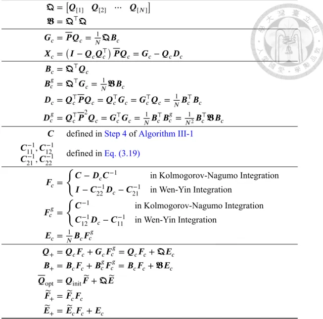
In this chapter, we optimize the Kolmogorov-Nagumo Integration (Algorithm III-1) and the Wen-Yin Integration (Algorithm III-2) for better performance, and propose algorithms based on the Gramian idea target for the case with many iterations. Table 3.1 lists the notations and the formulas used in this chapter. Here, we use bold italic uppercase letters (e.g.𝑨, 𝜴) for matrices, bold fraktur uppercase letters (e.g. 𝕭, 𝕼) for the matrices that keep unchanged in the iteration. Under-script𝑐 (e.g. 𝑸𝑐, 𝑿𝑐) are used for the matrices of the current iteration, and under-script plus sign (e.g.𝑩+, 𝑫+) are used for the matrices of the next iteration. Moreover, we use matrices with super-script𝑔 for the 𝑮𝑐 terms. For example, in the updating of𝑸+,𝑭𝑐 is the coefficient of𝑸𝑐, and𝑭𝑐𝑔 is the coefficient of 𝑮𝑐.
3.1 Optimization Problem
The integration stage finds an orthogonal matrix 𝑸 that best represent the orthonormal basis𝑸[1], 𝑸[2], … , 𝑸[𝑁]. Here, we define such best𝑸opt as
𝑸opt ∶= arg min
𝑸⊤𝑸=𝑰
1 𝑁
𝑁
∑𝑖=1‖𝑸[𝑖]𝑸⊤[𝑖]− 𝑸𝑸⊤‖
2
𝐹 . (3.1)
𝕼 = [𝑸[1] 𝑸[2] ⋯ 𝑸[𝑁]] 𝕭 = 𝕼⊤𝕼
𝑮𝑐= 𝑷 𝑸𝑐 = 𝑁1𝕼𝑩𝑐
𝑿𝑐= (𝑰 − 𝑸𝑐𝑸⊤𝑐) 𝑷 𝑸𝑐 = 𝑮𝑐− 𝑸𝑐𝑫𝑐 𝑩𝑐= 𝕼⊤𝑸𝑐
𝑩𝑐𝑔= 𝕼⊤𝑮𝑐 = 𝑁1𝕭𝑩𝑐
𝑫𝑐= 𝑸⊤𝑐𝑷 𝑸𝑐 = 𝑸⊤𝑐𝑮𝑐 = 𝑮⊤𝑐𝑸𝑐 = 𝑁1𝑩𝑐⊤𝑩𝑐 𝑫𝑐𝑔= 𝑸⊤𝑐𝑷2𝑸𝑐 = 𝑮⊤𝑐𝑮𝑐 = 𝑁1𝑩⊤𝑐𝑩𝑐𝑔 = 𝑁12𝑩𝑐⊤𝕭𝑩𝑐
𝑪 defined inStep 4ofAlgorithm III-1 𝑪11−1, 𝑪12−1
𝑪21−1, 𝑪22−1 defined inEq. (3.19) 𝑭𝑐=
{
𝑪 − 𝑫𝑐𝑪−1 in Kolmogorov-Nagumo Integration 𝑰 − 𝑪22−1𝑫𝑐− 𝑪21−1 in Wen-Yin Integration
𝑭𝑐𝑔= {
𝑪−1 in Kolmogorov-Nagumo Integration 𝑪12−1𝑫𝑐− 𝑪11−1 in Wen-Yin Integration
𝑬𝑐= 𝑁1𝑩𝑐𝑭𝑐𝑔
𝑸+= 𝑸𝑐𝑭𝑐+ 𝑮𝑐𝑭𝑐𝑔 = 𝑸𝑐𝑭𝑐+ 𝕼𝑬𝑐 𝑩+= 𝑩𝑐𝑭𝑐+ 𝑩𝑐𝑔𝑭𝑐𝑔 = 𝑩𝑐𝑭𝑐+ 𝕭𝑬𝑐 𝑸opt = 𝑸init𝑭 + 𝕼 ̃̃ 𝑬
𝑭̃+= ̃𝑭𝑐𝑭𝑐 𝑬̃+= ̃𝑬𝑐𝑭𝑐+ 𝑬𝑐
Table 3.1: Notations and Formulas Used in Optimization Integrations
The optimization problem is equivalent to a maximization problem
𝑸opt ∶= arg max
𝑸⊤𝑸=𝑰
1
2tr(𝑸⊤𝑷 𝑸) with 𝑷 ∶= 1 𝑁
𝑁
∑𝑖=1
𝑸[𝑖]𝑸⊤[𝑖]. (3.2)
Here, we define
𝑓 (𝑸) = 1
2tr(𝑸⊤𝑷 𝑸) (3.3)
as the objective function.
3.2 Improvements of Kolmogorov-Nagumo Integration
In the implementation, instead of explicitly forming𝑚 × 𝑚 matrices such as 𝑸𝑐𝑸⊤𝑐 (with 2𝑚2𝑙 flops), we compute 𝑙 × 𝑙 matrices such as 𝑸⊤[𝑖]𝑸𝑐 (with2𝑚𝑙2flops) to reduce com- putational cost and memory usage. For example,Step 3inAlgorithm III-1(Kolmogorov- Nagumo Integration) can be rewritten as
𝑿𝑐 = (𝐼 − 𝑸𝑐𝑸⊤𝑐) 𝑷 𝑸𝑐 = (𝐼 − 𝑸𝑐𝑸⊤𝑐)
⎛⎜
⎜⎝ 1 𝑁
𝑁
∑𝑖=1
𝑸[𝑖]𝑸⊤[𝑖]⎞
⎟⎟
⎠ 𝑸𝑐
= 1 𝑁
𝑁
∑𝑖=1
(𝐼 − 𝑸𝑐𝑸⊤𝑐) 𝑸[𝑖]𝑸⊤[𝑖]𝑸𝑐
= 1 𝑁
𝑁
∑𝑖=1
𝑸[𝑖]𝑸⊤[𝑖]𝑸𝑐− 1 𝑁
𝑁
∑𝑖=1
𝑸𝑐𝑸⊤𝑐𝑸[𝑖]𝑸⊤[𝑖]𝑸𝑐
= 1 𝑁
𝑁
∑𝑖=1
𝑸[𝑖](𝑸⊤[𝑖]𝑸𝑐) − 1 𝑁𝑸𝑐
𝑁
∑𝑖=1(𝑸⊤[𝑖]𝑸𝑐)
⊤
(𝑸⊤[𝑖]𝑸𝑐)
= 1 𝑁
𝑁
∑𝑖=1
𝑸[𝑖]𝑩[𝑖]− 1 𝑁𝑸𝑐
𝑁
∑𝑖=1
𝑩[𝑖]⊤𝑩[𝑖],
(3.4)
where𝑩[𝑖] = 𝑸⊤[𝑖]𝑸𝑐are𝑙×𝑙 matrices. Moreover, those matrix products can be accelerated by combining the matrices
ℵ[1]ℶ[1]+ ℵ[2]ℶ[2]+ ⋯ + ℵ[𝑁]ℶ[𝑁]= [ℵ[1] ℵ[2] ⋯ ℵ[𝑁]]
⎡⎢
⎢⎢
⎢⎢
⎢⎣ ℶ[1]
ℶ[2]
⋮ ℶ[𝑁]
⎤⎥
⎥⎥
⎥⎥
⎥⎦
. (3.5)
Therefore,eq. (3.4)can be rewritten as
𝑿𝑐 = 𝑮𝑐− 𝑸𝑐𝑫𝑐, (3.6)
where𝑮𝑐 = 𝑁1𝕼𝑩𝑐,𝑫𝑐 = 𝑁1𝑩𝑐⊤𝑩𝑐,
𝕼 = [𝑸[1] 𝑸[2] ⋯ 𝑸[𝑁]] and 𝑩𝑐 = [𝑩[1] 𝑩[2] ⋯ 𝑩[𝑁]] . (3.7)
Note that we may compute𝑩𝑐 as𝑩𝑐 = 𝕼⊤𝑸𝑐. Hence, the updating of 𝑸+ (Step 5in Algorithm III-1Kolmogorov-Nagumo Integration) can be written as
𝑸+ = 𝑸𝑐𝑪 + 𝑿𝑐𝑪−1 = 𝑸𝑐𝑪 + 𝑮𝑐𝑪−1− 𝑸𝑐𝑫𝑐𝑪−1 = 𝑸𝑐𝑭𝑐+ 𝑮𝑐𝑭𝑐𝑔, (3.8)
where
𝑭𝑐 = 𝑪 − 𝑫𝑐𝑪−1, 𝑭𝑐𝑔 = 𝑪−1. (3.9) Similarly, we can update𝑩+ = 𝕼⊤𝑸+ as
𝑩+ = 𝕼⊤𝑸+ = 𝕼⊤𝑸𝑐𝑭𝑐+ 𝕼⊤𝑮𝑐𝑭𝑐𝑔 = 𝑩𝑐𝑭𝑐+ 𝑩𝑐𝑔𝑭𝑐𝑔, (3.10)
where𝑩𝑐𝑔 = 𝕼⊤𝑮𝑐. Furthermore, instead of forming𝑿𝑐, we may compute𝜩 = 𝑿𝑐⊤𝑿𝑐 directly as
𝜩 = 𝑿𝑐⊤𝑿𝑐 = (𝑮⊤𝑐 − 𝑫𝑐𝑸⊤𝑐)(𝑮𝑐− 𝑸𝑐𝑫𝑐)
= 𝑮⊤𝑐𝑮𝑐− 𝑮⊤𝑐𝑸𝑐𝑫𝑐− 𝑫𝑐𝑸⊤𝑐𝑮𝑐+ 𝑫𝑐𝑸⊤𝑐𝑸𝑐𝑫𝑐
= 𝑮⊤𝑐𝑮𝑐− 𝑫𝑐𝑫𝑐− 𝑫𝑐𝑫𝑐+ 𝑫𝑐𝑫𝑐
= 𝑫𝑐𝑔− 𝑫𝑐2,
(3.11)
where𝑫𝑐𝑔 = 𝑮⊤𝑐𝑮𝑐 = 𝑁1𝑩𝑐⊤𝑩𝑐𝑔. Note that𝑸⊤𝑐𝑮𝑐 = 𝑮⊤𝑐𝑸𝑐 = 𝑫𝑐 and𝑸⊤𝑐𝑸𝑐 = 𝑰.
Algorithm III-4 Kolmogorov-Nagumo Integration (Optimized)
Require: 𝑸[1], 𝑸[2], … , 𝑸[𝑁](real𝑚 × 𝑙 orthogonal matrices), 𝑸init (initial guess).
Ensure: Integrated orthogonal basis𝑸opt.
1: Combine𝕼 = [𝑸[1] 𝑸[2] ⋯ 𝑸[𝑁]].
2: Initialize the current iterate𝑸𝑐 ← 𝑸init.
3: Assign𝑩𝑐 ← 𝕼⊤𝑸𝑐.
4: while (not convergent) do
5: Assign𝑮𝑐 ← 𝑁1𝕼𝑩𝑐,𝑩𝑐𝑔 ← 𝕼⊤𝑮𝑐,𝑫𝑐 ← 𝑁1𝑩𝑐⊤𝑩𝑐,𝑫𝑐𝑔 ← 𝑁1𝑩⊤𝑐𝑩𝑐𝑔.
6: Compute𝑪 ← (
𝑰
2 + (𝑰4 − 𝜩)1/2)
1/2
, where𝜩 = 𝑫𝑐𝑔− 𝑫𝑐2.
7: Assign𝑭𝑐 ← 𝑪 − 𝑫𝑐𝑪−1and𝑭𝑐𝑔 ← 𝑪−1.
8: Update𝑸𝑐 ← 𝑸𝑐𝑭𝑐+ 𝑮𝑐𝑭𝑐𝑔 and𝑩𝑐 ← 𝑩𝑐𝑭𝑐+ 𝑩𝑐𝑔𝑭𝑐𝑔.
9: end while
10: Output𝑸opt ← 𝑸𝑐.
3.3 Improvements of Wen-Yin Integration
Similar to the Optimized Kolmogorov-Nagumo Integration (Algorithm III-4), we combine the matrices𝕼 = [𝑸[1] 𝑸[2] ⋯ 𝑸[𝑁]] and define
𝑮𝑐 = 𝑷 𝑸𝑐 = 𝑁1𝕼𝑩𝑐, 𝑩𝑐 = 𝕼⊤𝑸𝑐,
𝑩𝑐𝑔= 𝕼⊤𝑮𝑐,
𝑫𝑐 = 𝑸⊤𝑐𝑷 𝑸𝑐 = 𝑸⊤𝑐𝑮𝑐 = 𝑮⊤𝑐𝑸𝑐 = 𝑁1𝑩𝑐⊤𝑩𝑐, 𝑫𝑐𝑔= 𝑸⊤𝑐𝑷2𝑸𝑐 = 𝑮⊤𝑐𝑮𝑐 = 𝑁1𝑩𝑐⊤𝑩𝑐𝑔.
(3.12)
We observed that𝑓 (𝑸𝑐) inStep 4ofAlgorithm III-2(Wen-Yin Integration) can be com- puted by
𝑓 (𝑸𝑐) = 12tr(𝑸⊤𝑐𝑷 𝑸𝑐) = 12tr(𝑁1𝑩𝑐⊤𝑩𝑐) = 2𝑁1 ‖𝑩𝑐‖2𝐹 . (3.13)
Moreover,‖𝑴‖2𝐹 can be written as
‖𝑴‖2𝐹 = tr(𝑴⊤𝑴) = tr((𝑸𝑐𝑮𝑐⊤− 𝑮𝑐𝑸⊤𝑐) (𝑮𝑐𝑸⊤𝑐 − 𝑸𝑐𝑮⊤𝑐))
= tr(𝑸𝑐𝑮⊤𝑐𝑮𝑐𝑸⊤𝑐 + 𝑮⊤𝑐𝑸⊤𝑐𝑸𝑐𝑮⊤𝑐 − 𝑸𝑐𝑮𝑐⊤𝑸𝑐𝑮⊤𝑐 − 𝑮𝑐𝑸⊤𝑐𝑮𝑐𝑸⊤𝑐)
= 2 tr(𝑮𝑐⊤𝑮𝑐) − 2 tr(𝑸⊤𝑐𝑮𝑐𝑸⊤𝑐𝑮𝑐) = 2 tr(𝑫𝑐𝑔) − 2 ‖𝑫𝑐‖2𝐹 .
(3.14)
To compute𝑸+, instead of explicitly forming𝑚 × 𝑚 matrix 𝑴 = 𝑮𝑐𝑸⊤𝑐 − 𝑸𝑐𝑮𝑐⊤, we construct two low-rank matrices [5]
𝑳 = [𝑮𝑐 𝑸𝑐] and 𝑹 = [𝑸𝑐 −𝑮𝑐] (3.15)
with𝑴 = 𝑳𝑹⊤. Using Woodbury matrix identity, the inverse can be rewritten as
(𝑰 −𝜏2𝑴)−1 = (𝑰 − 𝜏2𝑳𝑹⊤)
−1
= 𝑰 − 𝑳 (𝑹⊤𝑳 −2𝜏𝑰)−1𝑹⊤. (3.16)
Therefore,
𝑸+ = (𝑰 − 𝜏2𝑴)−1(𝑰 +𝜏2𝑴) 𝑸𝑐 =
(2 (𝑰 − 𝜏2𝑴)−1− 𝑰 )𝑸𝑐
= 𝑸𝑐− 𝑳 (12𝑹⊤𝑳 −1𝜏𝑰)−1𝑹⊤𝑸𝑐
= 𝑸𝑐− [𝑮𝑐 𝑸𝑐] 𝑪−1
⎡⎢
⎢⎣ 𝑸⊤𝑐
−𝑮⊤𝑐
⎤⎥
⎥⎦ 𝑸𝑐
= 𝑸𝑐− [𝑮𝑐 𝑸𝑐] 𝑪−1
⎡⎢
⎢⎣ 𝑰
−𝑫𝑐
⎤⎥
⎥⎦ ,
(3.17)
where
𝑪 = 1
2𝑹⊤𝑳 −1 𝜏𝑰 = 1
2
⎡⎢
⎢⎣ 𝑸⊤𝑐
−𝑮⊤𝑐
⎤⎥
⎥⎦
[𝑮𝑐 𝑸𝑐] − 1 𝜏𝑰
= 1 2
⎡⎢
⎢⎣
𝑸⊤𝑐𝑮𝑐 𝑸⊤𝑐𝑸𝑐
−𝑮⊤𝑐𝑮𝑐 −𝑮⊤𝑐𝑸𝑐
⎤⎥
⎥⎦
− 1 𝜏𝑰 = 1
2
⎡⎢
⎢⎣
𝑫𝑐− 2𝜏𝑰 𝑰
−𝑫𝑐𝑔 −𝑫𝑐− 𝜏2𝑰
⎤⎥
⎥⎦
(3.18)
is a2𝑙 × 2𝑙 matrix, which is much smaller than 𝑴. Denoting
𝑪−1 =
⎡⎢
⎢⎣
𝑪11−1 𝑪12−1 𝑪21−1 𝑪22−1
⎤⎥
⎥⎦
, (3.19)
eq. (3.17)becomes
𝑸+ = 𝑸𝑐− [𝑮𝑐 𝑸𝑐]
⎡⎢
⎢⎣
𝑪11−1 𝑪12−1 𝑪21−1 𝑪22−1
⎤⎥
⎥⎦
⎡⎢
⎢⎣ 𝑰
−𝑫𝑐
⎤⎥
⎥⎦
= 𝑸𝑐− 𝑮𝑐𝑪11−1+ 𝑮𝑐𝑪12−1𝑫𝑐− 𝑸𝑐𝑪21−1+ 𝑸𝑐𝑪22−1𝑫𝑐
= 𝑸𝑐(𝑪22−1𝑫𝑐− 𝑪21−1+ 𝑰) + 𝑮𝑐(𝑪12−1𝑫𝑐− 𝑪11−1)
= 𝑸𝑐𝑭𝑐+ 𝑮𝑐𝑭𝑐𝑔,
(3.20)
where
𝑭𝑐 = 𝑪22−1𝑫𝑐− 𝑪21−1+ 𝑰, 𝑭𝑐𝑔 = 𝑪12−1𝑫𝑐− 𝑪11−1. (3.21) Therefore, we can update𝑩+ = 𝕼⊤𝑸+as
𝑩+ = 𝕼⊤𝑸+ = 𝕼⊤𝑸𝑐𝑭𝑐+ 𝕼⊤𝑮𝑐𝑭𝑐𝑔 = 𝑩𝑐𝑭𝑐+ 𝑩𝑐𝑔𝑭𝑐𝑔. (3.22)