區域估測熱帶山地雲霧森林苔蘚附生植物生物量

(1)

國立臺灣大學理學院地理環境資源研究所碩士論文

Department of Geography College of Science National Taiwan University

Master Thesis

區域估測熱帶山地雲霧森林苔蘚附生植物生物量 Regional estimation of the biomass of epiphytic

bryophytes in a tropical montane cloud forest

賴冠宇 Guan-Yu Lai

指導教授：黃倬英博士 Advisor: Cho-ying Huang, Ph. D.

中華民國 108 年 7 月

July 2019

(2)

doi:10.6342/NTU201902408

(3)

誌謝

終於到了寫誌謝的時刻，能夠順利寫出論文真的是神的恩典！感謝神讓我在大一下學期因著對魔法森林般的棲蘭有強烈的好奇心，就一頭栽進黃倬英老師的研究室，真心覺得這是最適合我的研究室！首先，我要感謝指導教授黃倬英老師，

謝謝黃老師在我還是大學部學生的時候就用心栽培我，給我非常多出野外的機會，

逐漸培養我對棲蘭的愛；在碩班期間，謝謝老師協助我一步步釐清研究問題，更將許多國際期刊的英文寫作技巧傳授給我，且不厭其煩地協助我修改初稿。何其榮幸能成為老師指導的學生，感謝老師這六年來的指導與鼓勵！

謝謝國立臺灣師範大學的林登秋老師和林業試驗所的徐嘉君老師願意擔任論文口試委員，用心審查論文當中諸多的細節，並且給予我諸多寶貴的建議，讓後續論文修改能更加完善。謝謝森林系的關秉宗老師，一針見血點出我統計上的問題，

指點我R和統計分析上許多的疑難雜症，還有給予論文計畫書的建議，使得後續論文能進展順利。

謝謝朝夕相處每天都呼吸同一間空氣608的大家，從碩班申請和拓荒計畫剛開始執行就大力相挺的張雋、陪我出過最多次苔蘚調查也記錄最多棵樹的賸豐、讓棲蘭山屋變成高級西餐廳的鏡淵、給予我諸多ENVI和ArcGIS圖資和指導愷庭、時不時就揪打球團讓我可以好好紓壓一下的鴻錡、報帳行政一把罩有姊姊真好的婉瑜、超級認真遙測助教好搭檔欣儒、一起出過數不清例行的顯程、未來研究室新血宏祐、

時不時出現來關心大家的孝隆學長，以及給我許多統計建議的智昕學長。數不清到底一起出過幾次野外，雖然野外常常很狼狽很崩潰，但這些絕對都是很令人難忘的回憶。每兩個月一次的香料館，陪伴我度過兩年的碩班生涯！

謝謝所有曾經被我一起拉來拓荒計畫出野外的好朋友：大容、得笙、逸東、以理、昌典、唐詩、予佳、以恆以及大學部的學弟妹們，有你們一起出野外都會讓野外快樂一百倍！謝謝我的好朋友丞瑀、家禎，有妳們真好！謝謝北投禮拜堂的林立、阿貝、冠冠姐、黃義，常常關心我的論文進度，並為我守望代禱，做我的強力後盾。

謝謝阿詩總是為我加油打氣，用溫柔而堅定的語氣提醒我掌握進度，陪我一起禱告、聽我試講妳都聽不太懂的報告、與我討論統計分析。每一次的相聚都讓我充了飽飽電可以繼續努力下去，有你的支持真得很重要。

最後要謝謝我的家人，謝謝照顧我長大最疼我的阿嬤、每天用禱告為我守望甚至跟我一起出野外的媽媽、常請我吃大餐的姊姊、讓我帶木梯上棲蘭的爸爸、很關心我的陳碧霞阿姨，有你們的支持我才能完成學業，非常感謝！

賴冠宇謹誌

(4)

ii

摘要

附生苔蘚植物是中海拔熱帶山地雲霧森林最具代表性的物種之一，且在森林中的水循環、蒸發散扮演關鍵角色。其中，生物量是少數可間接估測附生苔蘚攔截霧水的參數，然而，附生苔蘚生物量調查至今依然缺乏兼具高效率、低成本且不具破壞性量化生物量的方式，區域尺度的估測更是困難。已知生物量與森林結構、物理環境和微氣候有高度相關性，透過現地調查以及遙測光達資料，我們可以間接估測區域尺度的附生苔蘚生物量。本研究分析區域尺度附生苔蘚生物量與46個生物物理、

地形以及氣候因子的關係，並評估在熱帶山地雲霧森林繪製區域尺度附生苔蘚生物量地圖的可行性。本研究樣區在臺灣東北部的棲蘭山 (24°35’N; 121°25’E, 16775 ha)，我們在六個林份跨海拔梯度 (1200-1950 m a.s.l.)，破壞性地蒐集131個100 cm² 附生苔蘚樣本，建立附生苔蘚厚度及生物量的異速生長迴歸模式。此外，我們設計一套新的高效率附生苔蘚生物量野外調查方法並使用所建立的迴歸模式，在另外 21個30 30公尺樣方估測樣區尺度附生苔蘚總生物量。最後使用偏最小平方迴歸分析影響附生苔蘚生物量空間分佈的顯著變量 (主成分)，並繪製區域尺度附生苔蘚生物量地圖。異速生長迴歸模式得指數為0.753有最佳結果 (r² = 0.72，p <0.001)，

樣區尺度估測平均附生苔蘚生物量 ( 標準偏差) 為188.7 100.3 kg ha^-1。偏最小平方迴歸結果顯示大樹密度、宿主胸高直徑、樹冠層高度、地上部生物量、海拔高度、剖面曲率、平面曲率、氣溫顯著影響附生苔蘚生物量的空間分佈。取前四個主成份共解釋94%的樣本變異，並繪製附生苔蘚生物量地圖。在區域尺度上估測平均附生苔蘚總生物量 ( 標準偏差) 為161.3 83.2 kg ha^-1，配合1 m空間解析度空載光達冠層高度模型與現地資料，估測棲蘭山的總附生苔蘚生物量為2808.6 Mg。本研究提出結合現地測量和空載光達資料的區域尺度繪圖方法，有助於評估附生苔蘚植物在熱帶山地雲霧森林水循環中的作用。

關鍵字：異速生長、臺灣扁柏、臺灣、遙測、光達、大尺度、偏最小平方迴歸

doi:10.6342/NTU201902408

(5)

Abstract

Epiphytic bryophytes are some of the key species characterizing mid-altitude tropical montane cloud forests (TMCF) and play a pivotal role in influencing the global hydrological cycle. For epiphytic bryophytes (EB), biomass is one of the only a few measurable parameters to assess the capacity of TMCFs to intercept fog. However, carrying out field EB measurements have known to be very technically challenging and time to carry out, which makes the regional quantification impractical. The abundance of EB is highly related to the forest structure, physical environment and microclimate.

Therefore, we may be able to indirectly map EB biomass at the regional scale by combining field observation and active remotely sensed light detection and ranging (lidar) spatial coverage. In this study, we investigated the relationship of the plot scale EB biomass and a comprehensive set of field and lidar derived biophysical, topographic and bioclimatic attributes and assessed the feasibility of regional mapping of EB biomass in a TMCF. The study was conducted in a 16773 ha TMCF of Chilan Mountain in the northeastern Taiwan. We destructively collected 131 100 cm² circular EB samples from six sites across an elevation gradient of 1200–1950 m a.s.l. to derive a general allometry of EB biomass using the central depth of each sample. Additionally, a new field instrument was designed specifically for the efficient estimation of EB biomass along tree stems, and the 30 30 m plot scale EB biomass (n = 21) was estimated with aids of previously measured in-situ field data and developed allometrics. The partial least squares regression was applied to investigate the relationship between the plot scale EB biomass and 46 field and/or lidar derived biophysical, topographic and bioclimatic attributes. The salient variables (principal components) were then selected to for regional mapping of EB biomass. The general allometric model had the best performance (r²= 0.72, p < 0.001)

(6)

iv

with the exponent of 0.753. Estimation of mean EB biomass ( standard deviation [sd]) at the plot-scale was 188.7 100.3 kg ha^-1. The partial least squares regression showed that big tree density, tree DBH, canopy height, aboveground biomass elevation, profile curvature, plan curvature and air temperature were significantly affecting spatial distribution of EB biomass. The first four principal components explaining 94% of data variation were used for regional EB biomass mapping. We estimated that the mean ( sd) EB biomass density was 161.3 83.2 kg ha^-1, and total EB biomass of the TMCF of Chilan Mountain is 2808.6 Mg. Our proposed synoptic sensing approach may be feasible for regional mapping of EB biomass, thereby advancing our understanding of the role of EB plays in the hydrological cycle of TMCFs.

Keywords: allometry, hinoki, lidar, large scale, partial least squares regression, synoptic sensing, Taiwan

doi:10.6342/NTU201902408

(7)

List of Figures

Figure 1 Study area.. ...5

Figure 2 Flow chart of the study.. ...9

Figure 3 A new instrument of epiphytic bryophytes biomass measurement.. ...12

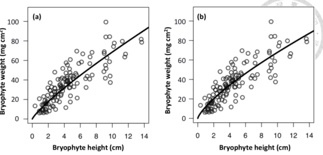
Figure 4 The general depth-biomass allometric regression model of epiphytic bryophytes. ...20

Figure 5 Standardized coefficients of 46 variables of partial least squares

regression ...25

Figure 6 Pearson correlation coefficient of components 1-4 with 46 variables in partial least squares regression.. ...26

Figure 7 Relationship between predicted TBB and measured TBB in partial least squares regression ...27

Figure 8 Predicted biomass of epiphytic bryophytes map on the Chilan

Mountain ...28

doi:10.6342/NTU201902408

(9)

List of Tables

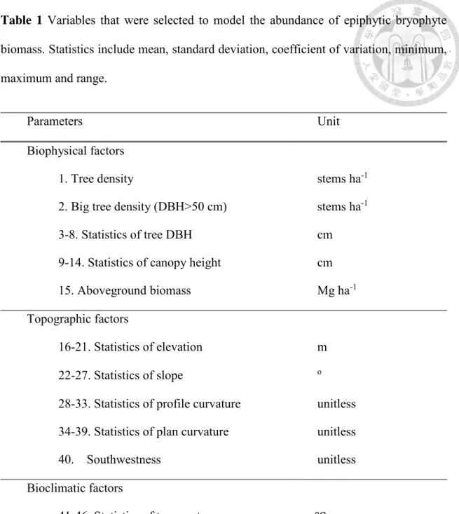
Table 1 Variables that were selected to model the abundance of epiphytic

bryophyte biomass ...17

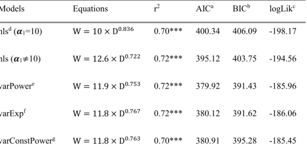
Table 2 Comparison of nonlinear regression results ...19

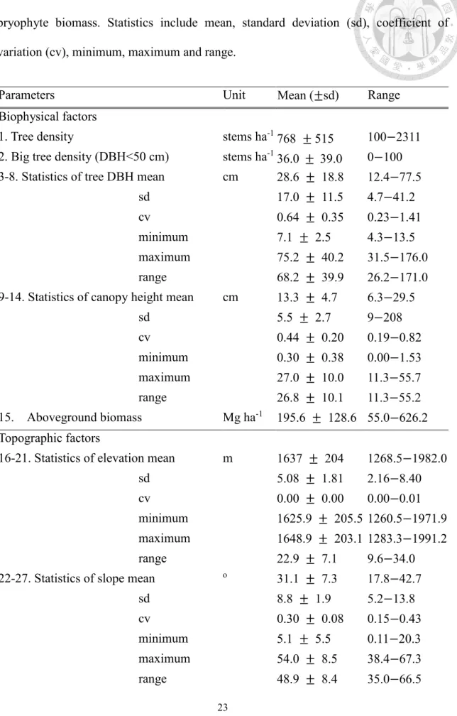
Table 3 Summary of variables that were selected to model the abundance of

epiphytic bryophyte biomass ...23

Table 4 Summary of relevant bryophytes biomass research. ...36

(10)

1

1. Introduction

Tropical montane cloud forests (TMCFs) are ecosystems experience frequent immersion of low altitude cloud (also known as “fog”, exchangeably used hereafter) with high humidity. TMCFs, by their names, are mostly distributed in the mountainous regions, and they play an areally unproportional role in the global terrestrial ecosystem functioning.

While covering only about 0.14% (~30M ha) of the Earth’s terrestrial surface (Bruijnzeel et al., 2011a) and 2.5% of tropical forests of the world (Bubb et al., 2004), they are the major water sources for lowland environments (mainly tropical forests). They are also responsible for one-third of the terrestrial net primary production and store approximately 40% of carbon in terrestrial vegetation (Bonan, 2008; Houghton, 2005; Saatchi et al., 2011) In addition, they are notable biodiversity hotspots of the biosphere (Luna-Vega et al., 2001). By intercepting parallel fog water, plants may obtain necessary water and nutrients for growth and maintain the health of the systems (Holwerda et al., 2010; Scholl et al., 2011; Stadtmüller, 1987). However, land use and cover change (Ray et al., 2006) and the prevailing global trend of elevated temperatures in the recent decades may alter regional climate and lift the presence of upslope fog (also known as cloud band) to higher elevation (Foster, 2001; Still et al., 1999).The change in bioclimate may directly modify the amount of cloud water and solar radiation yielded by TMCF and alter the microclimate, which may result in substantial impacts on the plants especially epiphytes (Benzing, 1998).

Epiphytes are some of the most representative plant species in TMCFs. (Barkman, 1958; Smith, 1982). They are rootless, and they maintain nutrients and water via photosynthesis or intercepting parallel fog water and vertical rainfall (Hofstede et al.,

doi:10.6342/NTU201902408

(11)

1993). In some TMCFs, high humidity harbors a large number of epiphytic bryophytes (EB). Epiphytic bryophytes are non-vascular terrestrial plants such as mosses, liverworts and hornworts. Most of the species lack stratum corneum preventing water from dispersing. They are very sensitive to the change in moisture due to their primitive physiological characteristics (Ah-Peng et al., 2017; Shi et al., 2017; Sillett et al., 2000).

They may also influence the global hydrological cycle by modifying parallel and vertical precipitation interceptions and evaporation (Chang et al., 2002; Porada et al., 2018;

Rhoades, 1995). Therefore, changes in the microclimate may have tremendous impacts on EB. In some systems, EB are keystone species for providing water and essential nutrients to maintain the health of TMCFs (Gradstein, 2008; Zotz & Bader, 2009).

However, quantification of the abundance of EB has been very challenging.

Biomass is one of the major metrics to indicate the abundance of plants (Bonham, 2013). For EB, biomass is also a key indirect parameter to assess the capacity of TMCFs to intercept fog (Zotz & Vollrath, 2003). The abundance of EB in TMCFs may be affected by microclimatic (e.g., humidity, temperature, luminosity) and host structural attributes (such as tree size, height, density) (Chen et al., 2010; Freiberg & Freiberg, 2000; Nöske et al., 2008; Peck et al., 1995). Field survey approaches such as destructively sampling with interpolation on the ground for low statured (Ah-Peng et al., 2017) or fallen trees (Chen et al., 2010), or uses of a ladder, a rope (Hsu et al., 2002; Nakanishi et al., 2016) a high tower or a crane (McCune et al., 1997; McCune et al., 2000) to reach tall trees were commonly implemented to measure EB biomass. However, field EB measurements have known to be very challenging to carry out, which makes the regional quantification impractical (Barker & Pinard, 2001; Moffett & Lowman, 1995).

(12)

3

Remote sensing has been widely utilized to map vegetation characteristics of different biomes (Crowther et al., 2015; DeFries, 2008; Vicente-Serrano et al., 2013).

Airborne light detection and ranging (hereafter lidar) has been widely used to delineate forest structural parameters at the high spatial resolution such as tree height, canopy depth and biomass (Asner et al., 2010; Lefsky et al., 2002; Saatchi et al., 2011). In addition, pulsed laser beams can penetrate the canopy layers to the ground level and delineate the beneath topography (Haugerud et al., 2003), which may be utilized to interpolate the forest microclimate (Jucker et al., 2018). Furthermore, the continuous coverage of canopy height (known as the canopy height model [CHM]) may be derived by subtracting the bottom (the digital elevation model, DEM) from the top (the digital surface model, DSM) of the spatial layers (Lefsky et al., 2005). Therefore, in this study, we derived comprehensive sets of bioclimatic, biophysical and topographic attributes by integrating field and lidar data (1) to investigate salient factors that govern the abundance of EB; (2) to develop a spatial explicit model to map EB biomass of a TMCF at the regional scale.

doi:10.6342/NTU201902408

(13)

2. Methods and Materials

2.1 Study area

The study focused on a 16,773 ha TMCF of Chilan Mountain (24^o98’N, 120^o97’E) in the northeastern Taiwan (see the definition of TMCF in Schulz et al. 2017) (Figure 1). The precipitation in summer and winter are mostly orographic precipitation and the typhoons and the northeastern monsoon, respectively. Annual precipitation and mean temperature of the site are 4,000 mm y^-1 and 12.7°C, respectively. The mean ( standard deviation [sd]) elevation of the site is 1680 343 m a.s.l., and mean slope ( sd) is 38.2° 13.4°

ranging from 0° to 88.7°. The rugged terrain faces regular moist wind from the Pacific Ocean resulting in frequent occurrence of upslope fog approximately 300+ days of a year and 38% of the time (Lai et al., 2006). The humid bioclimate harbors a substantial amount of EB. There were 49 and 24 species observed in mature old-growth and regenerated forests, respectively, by a preliminary inventory (Chang et al., 2002). The primary vegetation type of the TMCF is conifer forest, dominated by hinoki cypress (Chamaecyparis obtusa var. formosana) and Japanese cedar (Cryptomeria japonica).

(14)

5

Figure 1 Study area. (a, b) The study area was located in the northeast Taiwan (24^o98’N, 120^o97’E). Six forest stands were selected for EB biomass allometric model development (yellow dots), twenty-one 30 × 30 m inventory plots were selected for plot-scale EB estimation (red triangle) and four meteorological stations were installed for air temperature data collections (orange star) along the forest routes (the blue lines). (c) The dominant tree species are Taiwan hinoki cypress and Japanese cedar forest with tree age range from 30 to 100 years. (d) The dominant species of epiphytic bryophytes are Bazzania, accounting for 78% of the total EB coverage.

doi:10.6342/NTU201902408

(15)

2.2 Field EB biomass sampling and model development

Complete procedures and analyses of this study are summarized in Figure 2. The first step was to derive a general allometry for EB biomass, and six forest stands along the elevation gradient of 1200–1950 m a.s.l. were selected (Figure 1). In the summer (May- October) of 2017, the center depth of each EB of the same species (n = 131) within a 100 cm² circularly shaped frame found below 3 m from the ground was measured using a stainless ruler and destructively sampled. The samples were stored in sealed polyethylene-linear low density bags to keep moist and were placed in an ice box.

Samples were transported to a laboratory within eight hours after removing from host trees. Soils and tree barks attached to the samples were cleaned using tap water before drying them in a 70℃ biomass oven for at least 72 hours and weighed them using a three decimal point electronic balance (LIBROR EB-430H, Shimadzu, Japan). In this study, EB biomass was defined as the total sampled dry weight divided by the projected surface area of the sample (mg cm^-2). The depth of EB was used as a unique trait for each independent sample, and we developed EB biomass allometric equations which explored the relationship between the weight and the depth (Eq. 1):

W = 𝛼1 × 𝐷^𝛽¹, (1)

where W is the EB biomass per unit area (mg cm^-2), D is the EB depth (cm), and 𝛼1 and β1 are the coefficient and is exponent components, respectively. A power model was selected by referring to Chen et al. (2010). Continuous values ranging from 0.01 to 2.0 with an interval of 0.01 were selected for β1 to derive an optimized model of fitting the empirical data based on generalized least squares (GLS) to minimize the effect of the unequal variances effects which were commonly observed in ecological data. Three

(16)

7

variance covariate functions were used to involve regression of the fitted values and the residuals within the fitted model including exponential of a variance covariate (varExp), power of a variance covariate (varPower) and constant plus power of a variance covariate (varConsPower). All statistical analyses were conducted using the “nlme” (Pinheiro et al., 2013) package in R 3.5.0 (Team, 2013).

doi:10.6342/NTU201902408

(17)

(18)

9

Figure 2 Flow chart of the study. This study initiated the three steps to achieve the two goals. (1) To develop the relationship between EB depth and weight, six forest stands on Chilan Mountain were selected for field sampling and modeling; (2) to estimate total EB biomass (TBB) at the plot scale, twenty-one 30 × 30 m plots along the elevation gradient; (3) to investigate salient factors that govern the abundance of EB, the bioclimatic, biophysical and topographic variables were compiled for partial least squares regression analysis. Finally, we could estimate and map the total EB biomass over a vast region.

doi:10.6342/NTU201902408

(19)

2.3 The plot-scale EB biomass estimation

Twenty-one 30 × 30 m plots along the elevation gradient of 1260–1990 m a.s.l were selected for estimating total EB biomass (TBB) at the plot scale (Figure 1). Diameter at breast height (DBH) of 16 plots measured at 130 cm above the ground for each living tree (DBH 5 cm) within the plot was recorded in July of 2016. The same surveying protocol was applied on five more plots during January of 2019. During May-August of 2018 and January-February of 2019, we selected 10 trees evenly distributed along the DBH gradient of each plot (n = 210) to interpolate the plot scale EB biomass. Moreover, the basal diameter of each sampled tree was also measured, and the relationship between basal area and DBH was investigated.

A new field instrument was designed specifically for the estimation of EB biomass (Figure 3). From the ground surface to 3 m in each sampled tree stem height, the EB depths (including the absence of EB with the depth of 0 cm) were recorded every 30 cm in different orientations, and the data were averaged as the mean EB depth of the sampled stem surface area. We note that all trees in the plots were taller than 3 m. The sample trees with DBH larger than 20 cm were recorded in eight directions (north, northeast, east, southeast, south, southwest, west and northwest) otherwise in four initial four cardinal directions. The stem below 1.3 m from the ground was truncated cone shape and from 1.3 m to the top of the sampled height (3 m from the ground) was a cylinder. Therefore, the surface area (cm²) of stem below 3 m (“sampled stem area” hereafter) was calculated by referring to Eqs.2 and 3,

SA = 170 × π × 𝐷𝐵𝐻 + 𝜋 × ℓ × (^𝐵𝐷₂ +^𝐷𝐵𝐻₂ ), (2)

(20)

11

ℓ = √130²+ (^𝐵𝐷₂ −^𝐷𝐵𝐻₂ )² , (3)

where BD and DBH are basal diameter (cm) and diameter at breast height (cm), respectively. With the knowledge of the EB biomass allometry (Eq. 1) and the EB depth per unit area of each measured point below 3 m from the ground in each direction, we may be able to estimate the EB biomass per unit. Cover area (cm²) was calculated from sampled stem area by multiplying EB coverage. With the cover area of EB and the biomass per unit, we should be able to estimate the EB biomass within the sampled stem area. The EB biomass of the sampled stem area was then exterpolated to it of the entire individual tree by multiplying a coefficient of 0.45 × ln 𝐷𝐵𝐻 to convert EB biomass below 3 m from the ground to EB biomass of the entire individual tree by referring to the in-situ destructive measurement by scrapping EB from 10 harvested hinoki trees (Deng,

2006). Finally, EB biomass of the sampled stem area was then interpolated to it of the entire plot with the knowledge of DBH and DBH-BD of each tree and we could interpolate the total EB biomass (TBB) of the entire plot.

doi:10.6342/NTU201902408

(21)

Figure 3 A new instrument of epiphytic bryophytes biomass measurement. (a) Sling ropes were hang down at 3 m above the ground. (b) The EB depths including the absence of EB with the depth of 0 cm were recorded every 30 cm in different orientations and the sample trees with DBH larger than 20 cm were recorded in eight directions (north, northeast, east, southeast, south, southwest, west and northwest) otherwise in four initial four cardinal directions. The dendrometer was installed at 130 cm above the ground.

(22)

13

2.4 Airborne lidar

The airborne lidar data were acquired using Leica ALS60 (Leica Geosystems AG, Heerbrugg, Switzerland) and Optech ALTM Pegasus (Teledyne Optech, Toronto, Canada) systems in 2014 via a national scale geological inventory project administered by the Taiwan Central Geological Survey. The original point cloud data were preprocessed at the point cloud density of 1.5 points per square meter and resampled to a 1-m spatial resolution by the data provider. According to the data user manual (Hou et al., 2014), 40%

or greater overlap was required for each neighboring flight stripe. The lidar first return and ground points were interpolated using adaptive kriging (SCOP++, Department of Geodesy and Geoinformation, Vienna, Austria) to generate DEM and DSM, and consequently canopy height model (hereafter CHM). The accuracy of the lidar product was 22.5 cm as compared with measurements from a high precision GPS; the quality was visually assessed to verify potential erroneous point cloud data, such as extremely high or low values compared to values of the nearby features before data product distribution (Hou et al., 2014).

doi:10.6342/NTU201902408

(23)

2.5 Field meteorological data

Monthly air temperatures of the study site from January to December of 2018 were acquired (EM50 data logger, ICT international, Pullman, USA) by four open-sky meteorological stations (1151 m, 1514 m, 1650 m and 1811 m a.s.l.) (Figure 1). The data were originally recorded every two minutes and were averaged to the monthly resolution.

The lapse rate of monthly temperature along the elevation of the study region was estimated by comparing the concurrent data with the spatially corresponding elevations.

Monthly air temperatures of 21 sampling plots were interpolated by referring to the data from the nearest meteorological station and the estimated regional lapse rate.

(24)

15

2.6 Regional estimation of EB biomass

We compiled a set of plot scale biophysical, topographic and bioclimatic attributes to investigate the determinants that may influence the abundance of EB biomass in Chilan Mountain, and may facilitate regional mapping of EB biomass. There were total 41 variables defined (Table 1) and may be generalized as three broad categories: Biophysical, topographic and bioclimatic factors. For the biophysical factor category, the tree density and the big tree density were the total tree counts of living trees (DBH 5 cm) and the large ones (arbitrarily defined as DBH 50 cm by referring to our plot inventory data) within the field plots and were scaled to the hectare scale, respectively. Aboveground biomass (AGB) of hinoki and Japanese cypress (JC) were estimated using species specific allometrics (Duh et al., 2011; Huang et al., 2012):

ln 𝐴𝐺𝐵hinoki = −2.3723 + 2.3385 × ln(𝐷𝐵𝐻), (4)

ln 𝐴𝐺𝐵JC = −1.8460 + 2.1832 × ln(𝐷𝐵𝐻). (5)

Basic statistics (mean, sd, coefficient of variation [CV], max, min and range) of field measured tree DBH and lidar derived CHM were calculated using R 3.5.0 and ArcGIS v.

10.4 (Environmental Systems Research Institute, Inc., Redlands CA, USA), respectively.

Basic statistics of topography (elevation [m], slope [°], curvature [unitless]) were acquired/calculated from lidar DEM using ArcGIS. Curvature displays the shape of the slope and was calculated by computing the second derivative of the surface. The profile curvature affects the acceleration and deceleration of flow and the plan curvature influences convergence and divergence of flow. Aspect is not incremental (1° and 359°

are both north facing slopes), and a numerical metric southwestness (cos(aspect-255°))

doi:10.6342/NTU201902408

(25)

was computed to indicate the intensity of solar radiation (aridity; values of 1 and -1 for southwest and northeast aspects, respectively) of each plot in this region (Wang et al., 2016).

All attributes were standardized to investigate the salient attributes for the estimation of TBB in Chilan Mountain using partial least squares regression (hereafter PLSR) methods. The PLSR is presented as an iterative algorithm that decomposes the dependent variables x into the product of a set of orthogonal factors and specific loadings to confront multicollinearity and relatively few samples (Abdi, 2003). The root mean squared error of prediction (RMSEP) was used to quantify the amount of variation explained by the developed relationships and the accuracy of the PLSR by using cross-validated leave- one-out (LOO) segments. The decision on how many components was based on the approach “onesigma” to calculate the standard deviation of the cross-validated residuals that consisted of choosing the model with fewest components. The PLSR statistical analysis was conducted using the “pls” (Mevik & Wehrens, 2015) package in R. Finally, we selected the potential attributes to map the TBB at the regional scaleusing ArcGIS.

(26)

17

Table 1 Variables that were selected to model the abundance of epiphytic bryophyte biomass. Statistics include mean, standard deviation, coefficient of variation, minimum, maximum and range.

Parameters Unit

Biophysical factors

1. Tree density stems ha^-1

2. Big tree density (DBH>50 cm) stems ha^-1 3-8. Statistics of tree DBH cm 9-14. Statistics of canopy height cm 15. Aboveground biomass Mg ha^-1 Topographic factors

16-21. Statistics of elevation m 22-27. Statistics of slope ^o

28-33. Statistics of profile curvature unitless 34-39. Statistics of plan curvature unitless

40. Southwestness unitless

Bioclimatic factors

41-46. Statistics of temperature ℃

doi:10.6342/NTU201902408

(27)

3. Results

3.1 Epiphytic bryophytes biomass allometry

In the summer (May-October) of 2017, the 100 cm² circular shaped sample EB samples (n = 131) were collected in six forest stands of Chilan Mountain (Figure 1). The mean ( sd [minimum–maximum]) sampled EB depth and biomass were 4.5 2.9 cm (0.3–13.7 cm) and 36.0 20.3 (6.2–99.3) mg cm^-2, respectively. Significant positive correlations (p

< 0.005) were found among EB depth and weight according to the analysis (Table 2). The performance of allometric equation of the power of variance covariate function (r²= 0.72, AIC = 380, p<0.0001) was superior to other models with coefficient and exponent of 11.96 and 0.753, respectively (Figure 4) The standardized residuals were evenly distributed compared to which in equations without calibration (Figure S1).

(28)

19

Table 2 Comparison of nonlinear regression results. The performance of allometric equation of the power of variance covariate function was superior to other models with coefficient and exponent of 11.96 and 0.753. The AIC and BIC of the models calibrated by generalized least squares were lower than ones of the first two models without calibration.

Models Equations r² AIC^a BIC^b logLik^c

nls^d (𝜶1=10) W = 10 × D^0.836 0.70*** 400.34 406.09 -198.17 nls (𝜶1≠10) W = 12.6 × D^0.722 0.72*** 395.12 403.75 -194.56

varPower^e W = 11.9 × D^0.753 0.72*** 379.92 391.43 -185.96

varExp^f W = 11.8 × D^0.767 0.72*** 380.12 391.62 -186.06 varConstPower^g W = 11.8 × D^0.763 0.70*** 380.91 395.28 -185.45

a: Akaike information criterion; b: Bayesian information criterion; c: Log likelihood; d: Nonliear squared regression; e: Power of a variance covariate; f: exponential of a variance covariate; g: Constant power of a variance covariate; *** P value of model < 0.001

doi:10.6342/NTU201902408

(29)

Figure 4 The general depth-biomass allometric regression model of epiphytic bryophytes (Eq. 1) (a) The model was established by setting 𝛼1≠10 without calibration; (b) The best performance of allometric equation of the power of variance covariate function (r²= 0.72, AIC = 380, p<0.0001) was superior to other models with coefficient and exponent of 11.96 and 0.753.

(30)

21

3.2 The plot-scale EB biomass estimation

Diameter of breast height of 1451 trees were measured within 21 plots was recorded in July of 2016 and January of 2019. The mean ( sd [minimum–maximum]) DBH of total trees within twenty-one plots was 20.3 17.5 cm (5.0–176.0 cm (n = 1451, Figure 1)).

The EB investigation of 210 trees within twenty-one plots were investigated. The mean ( sd [minimum–maximum]) DBH and BD of sampled trees (n = 210) were 33.5 27.8 (7.6–128.7) and 48.5 33.8 (9.9–186.2) cm, respectively. The measured DBHs and basal diameters were very highly correlated (R²= 0.97, p < 0.0001) and the BD-DBH ratio was 1.37. With this information, we computed the sampled stem areas in the plots by referring to Eq. 2. The mean ( sd [minimum–maximum]) sampled stem area per tree was 3.4 2.7 (0.81–13.5) cm², and EB biomass for each tree within the plots was estimated (0.9 1.6 [0.00–9.1]) kg by the in-situ conversion coefficient (Deng, 2006). Finally, TBB of each plot can be interpolated, and the mean ( sd [minimum–maximum]) total EB biomass at the plot-scale (n = 21) was 188.7 100.3 (49.9–408.5) kg ha^-1.

doi:10.6342/NTU201902408

(31)

3.3 Regional EB estimation

A set of plot scale biophysical, topographic and bioclimatic attributes were compiled to investigate the determinants that may influence the abundance of EB biomass in Chilan Mountain (Table 3, Figure S2) using PLSR. For the TBB estimated within 1-4 components, the RMSEPs were ranging from 87.6 to 80.7 kg ha^-1 (Figure S3) and 50-94%

of the total TBB cumulative variance were explained. Overall, the biophysical and topographic attributes were positively related to TBB, and the bioclimatic attributes were overall negatively related to TBB (Figure 5). Considering the correlation of components 1-4 with 46 variables in PLSR, the elevation (mean, SD, maximum, minimum), profile curvature (SD), plan curvature (SD, range) and air temperature (mean, CV, maximum, minimum) were the salient variables explaining 50% variance of TBB in the first component (p < 0.001, Figure 6); the big tree density, tree DBH (SD, maximum, range), CHM (mean, SD) and aboveground biomass were the salient variables in the second and third components explaining 24% and 11% variance of TBB, respectively (p < 0.001, Figure 6). To assess the performance of the regression equations, the predicted TBB obtained from the PLSR equation were compared with the measured TBB acquired from field data (n = 21). The results showed that the predicted TBB was consistent with the measured TBB (R² = 0.94, p < 0.001) along the 1:1 line (Figure 7) and the PLSR model may be used to for regional TBB estimation in TMCF of Chilan Mountain. The model estimated that TBB of the study regional was 2808.6 Mg. The mean ( sd [minimum–

maximum]) regional EB estimation in Chilan Mountain was 161.3 83.2 (0-650.0) kg ha^-1(Figure 8).

(32)

23

Table 3 Summary of variables that were selected to model the abundance of epiphytic bryophyte biomass. Statistics include mean, standard deviation (sd), coefficient of variation (cv), minimum, maximum and range.

Parameters Unit Mean (±sd) Range

Biophysical factors

1. Tree density stems ha^-1 768 ± 515 100−2311 2. Big tree density (DBH<50 cm) stems ha^-1 36.0 ± 39.0 0−100 3-8. Statistics of tree DBH mean cm 28.6 ± 18.8 12.4−77.5 sd 17.0 ± 11.5 4.7−41.2 cv 0.64 ± 0.35 0.23−1.41 minimum 7.1 ± 2.5 4.3−13.5 maximum 75.2 ± 40.2 31.5−176.0 range 68.2 ± 39.9 26.2−171.0 9-14. Statistics of canopy height mean cm 13.3 ± 4.7 6.3−29.5 sd 5.5 ± 2.7 9−208 cv 0.44 ± 0.20 0.19−0.82 minimum 0.30 ± 0.38 0.00−1.53 maximum 27.0 ± 10.0 11.3−55.7 range 26.8 ± 10.1 11.3−55.2 15. Aboveground biomass Mg ha^-1 195.6 ± 128.6 55.0−626.2 Topographic factors

16-21. Statistics of elevation mean m 1637 ± 204 1268.5−1982.0 sd 5.08 ± 1.81 2.16−8.40 cv 0.00 ± 0.00 0.00−0.01 minimum 1625.9 ± 205.5 1260.5−1971.9 maximum 1648.9 ± 203.1 1283.3−1991.2 range 22.9 ± 7.1 9.6−34.0 22-27. Statistics of slope mean ^o 31.1 ± 7.3 17.8−42.7 sd 8.8 ± 1.9 5.2−13.8 cv 0.30 ± 0.08 0.15−0.43 minimum 5.1 ± 5.5 0.11−20.3 maximum 54.0 ± 8.5 38.4−67.3 range 48.9 ± 8.4 35.0−66.5

doi:10.6342/NTU201902408

(33)

28-33. Statistics of profile curvature mean unitless -0.06 ± 1.5 -2.8−2.9 sd 20.1 ± 4.1 13.8−31.0 cv -19.2 ± 49.9 -165.0−41.0 minimum -88.3 ± 33.7 -157.7−0.13 maximum 104.6 ± 36.6 60.6−215.4 range 192.9 ± 63.0 78.3−373.2 34-39. Statistics of plan curvature mean unitless -0.05 ± 1.2 -1.8−2.4 sd 20.3 ± 5.0 13.7−32.9 cv -7.3 ± 35.5 -76.5−52.8 minimum -97.0 ± 31.1 -152.3−-52.1 maximum -93.3 ± 37.1 46.4−172.4 range 190.2 ± 60.0 102.4−317.6 40. Southwestness unitless 0.05 ± 0.65 -1.0−1.0 Bioclimatic factors

41-46. Statistics of temperature mean ^oC 13.8 ± 0.9 12.2−15.4 sd 4.5 ± 0.1 4.4−4.8 cv 0.33 ± 0.02 0.30−0.36 minimum 6.4 ± 0.9 5.0−8.0 maximum 19.1 ± 1.0 17.1−20.8 range 12.6 ± 0.3 12.1−13.4

(34)

25

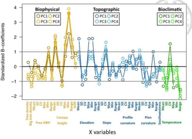
Figure 5 Standardized coefficients of 46 variables of partial least squares regression.

Overall, considering the first fourth component, the biophysical (brown circles) and topographic (blue circles) attributes were positively related to the total bryophytes biomass, and the bioclimatic attributes (green circles) were negatively related to the total bryophytes biomass.

doi:10.6342/NTU201902408

(35)

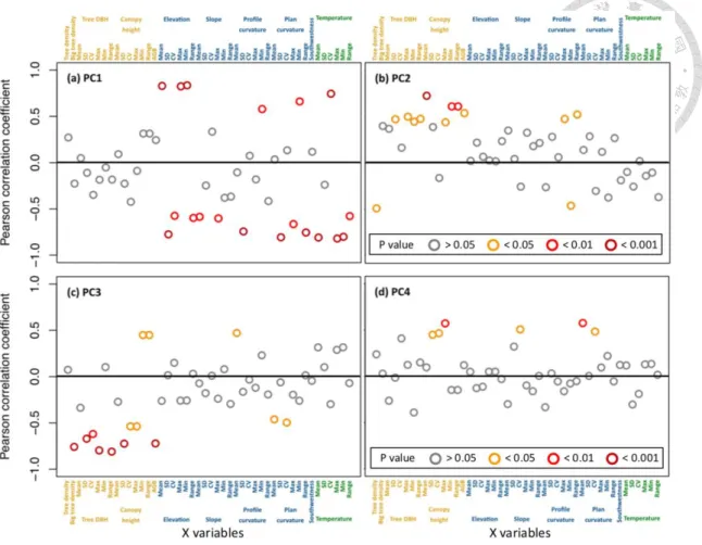
Figure 6 Pearson correlation coefficient of components 1-4 with 46 variables in partial least squares regression. In the first component, the elevation (mean, standard deviation [SD], minimum, maximum), profile curvature (SD), plan curvature (SD, range) and air temperature (mean, coefficient of variation [CV], minimum, maximum) were the salient variables. In the second component, the tree density, DBH (sd, minimum, maximum, range), canopy height (mean, minimum, maximum, range), aboveground biomass, profile curvature (minimum, maximum, range) were the salient variables. In the third component, big tree density, DBH (sd, cv, maximum, range), canopy height (sd, cv, minimum, maximum, range), aboveground biomass, profile curvature mean and plan curvature (mean and cv) were the salient variables. In the fourth component, canopy height (sd, cv, maximum), slope mean and plan curvature (mean, cv) were the salient variables.

(36)

27

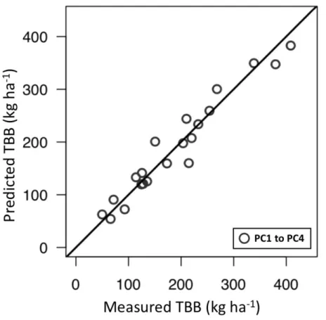
Figure 7 Relationship between predicted TBB and measured TBB in partial least squares regression. The first four principal components explaining 94% of data variation were used for regional EB biomass mapping.

doi:10.6342/NTU201902408

(37)

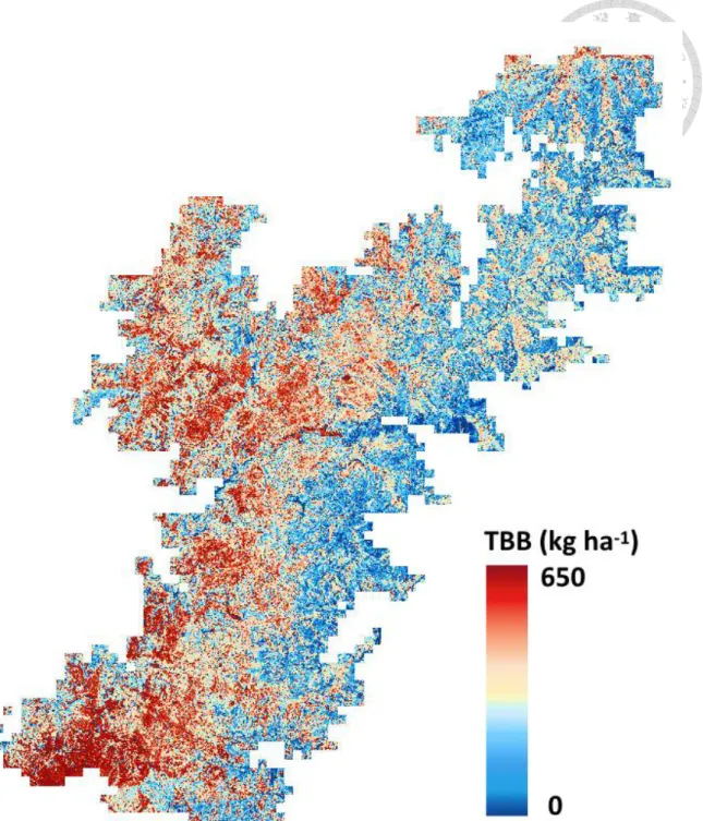
Figure 8 Predicted biomass of epiphytic bryophytes map on the Chilan Mountain. We estimated that the mean ( sd) EB biomass density was 161.3 83.2 kg ha^-1, and total EB biomass of the TMCF of Chilan Mountain is 2808.6 Mg by first four components in PLSR.

(38)

29

4. Discussion

Epiphytic bryophytes are some of the key species characterizing mid-altitude tropical montane cloud forests (Bruijnzeel et al., 2011b) and play a pivotal role in influencing the global hydrological cycle (Porada et al., 2018). Due to the morphology of the species, it is very difficult to quantify the abundance. In this study, we demonstrate that it may be possible for regional mapping EB biomass. However, challenges and uncertainties remain and need to be assessed. Our discussion will mainly focus on (1) EB depth-biomass allometry; (2) scaling of EB biomass from the patch to forest stand scales; (3) determinants governing the abundance of EB and (4) remotely sensed regional EB biomass estimation.

doi:10.6342/NTU201902408

(39)

4.1 Epiphytic bryophytes depth-biomass allometry

Plant allometry focuses on relationships between plant body size and biomass, production, population density or other dependent variables (Enquist et al., 1998; Enquist et al., 1999).

Stanton and Reeb (2016) pointed out that some characteristics of bryophytes may be allometrically scaled like vascular plants. However, it may not be applicable to all species.

In this study, in-situ general allometric equations were developed to estimate EB biomass using the central depth of sampled 100 cm² circular patch. The mean exponent of the power models of these five equations was 0.75 (3/4) ranging from 0.72 to 0.83 (Table 2), which agrees with the 3/4 power law (Kleiber, 1947) and is similar to the constant scaling exponents over a wide range of vascular plant size often with a quarter-powers in metabolic scaling theory (West et al., 1997, 1999). However, epiphytic bryophytes are non-vascular plants which compose of a simple stem has only a limited role in transporting moisture and nutrients through conducting tissues and they do not follow the vascular transport system as a self-similar, fractal-like branching network (Ligrone et al., 2000). Two major branching forms in bryophytes are sympodial with connected modules of same level and monopodial (Stanton & Reeb, 2016). For most vascular plants, the branching bifurcation is two (Enquist et al., 2007), and the height is 1/4 exponent of mass (West et al., 1999), which was different to our empirical observation. This verifies that the basic assumption of self-similar branching network of an organism plays a major role in governing the allometric relationship.

(40)

31

4.2 Scaling of EB biomass from the patch to forest stand scales

It is extremely challenging to non-destructively measure EB biomass, and a new field approach was invented in this study (Figure 3). This is crucial since it could take many years for EB to recover (Fenton et al., 2003). In addition, the approach was efficiently, which may permit fast sampling for a large region. This study focuses on the height below 3 m where the majority of EB are present (Trynoski & Glime, 1982). The sampled area may be further extended with aids of foldable ladder or tree climbing. With the availability of previously derived in-situ ratio of biomass of the sampled area and the total area of a tree, we may be able to estimate EB biomass at the individual tree and the plot scales. This sampling approach should be reliable and the models explained 72% of data variation (Figure 4). The performances were satisfactory since only a single variable (the central depth of a sample) was used to model biomass of EB with variable morphologies.

In this study, assumptions were made that the sample circular areal size of 100 cm² was appropriate and the central depth was representative, and these should be further investigated especially for the latter one. In some cases, plant depths within the circular shaped frame were not uniform mostly due to the variation in the abundance. In some rare cases, more than one species were present within the sampling, which were not visible on site. Hence, the use of central depth could be dubious and may induce model uncertainty. At the tree scale, the distribution of EB biomass on a tree was influenced by microclimate positions and directions. Therefore, we calculated the depth of EB in four and eight directions for small and large trees, respectively, which may reduce microclimate-induced biases (Figure S4). As we extrapolated EB biomass of an entire tree, an in-situ unfixed coefficient was applied to convert EB biomass of the sampled stem area to EB biomass of an entire tree. One potential research limit is that the tree

doi:10.6342/NTU201902408

(41)

scale EB biomass estimation, which was extrapolated from it of the sampled tem area and was interpolated to the plot scale, was not validated. This requires tree climbing or destructive harvesting to clear EB of entire trees. Unfortunately, there was no availability of the support of tree climbing. Logging in nature forests has been completely forbidden in Taiwan since 1991. Therefore, the latter option may not be possible due to the local regulation. In the future, we might be able to take the advantage of tropical cyclone- induced fallen logs and harvest EB biomass at the ground level.

(42)

33

4.3 Determinants governing the abundance of EB

In this study, we compiled a large set of biophysical, topographic and bioclimatic factors derived from field and airborne lidar data to investigate salient factors that govern the abundance of EB in TMCF of Chilan Mountain in northern Taiwan. For biophysical determinants, as expected, the parameters that were related to tree size (aboveground biomass, DBH and CHM) were positively related to TBB. The larger DBH of host tree provide more diverse micro-habitats for EB succession resulting from different bark structure, trunk chemical composition, humidity and luminosity (Chen et al., 2010). We note that data of a small portion (2 of the 21 [11%]) of the field plots (plot FR170 and Neighbor) with high biomass density (≥330 Mg ha^-1) deviated from the main pattern, and negative trends of TBB and aboveground biomass, DBH and CHM were observed (Figure S5). This suggests that there may be a threshold for the positive relationship between TBB and tree size at the upper end. Sites with extremely high carbon storage of this study region may be characterized as relatively lower and the higher luminosity resulting in a desiccative micro-habitat and harbored fewer TBB.

For topographic attributes, TBB generally increased with elevation in 50% of the surveyed plots. The finding agreed with Wolf (Wolf, 1993) with the estimation of bryophyte biomass across an elevation gradient in Andes. However, intuitively, lower elevations of the TMCFs within the cloud band should experience more daily upslope fog from moist wind from the Pacific Ocean, and may be able to harvest sufficient cloud water in the study region. The complex relationships among slope, profile curvature, plan curvature and TBB were difficult to decipher (Werner et al., 2012). The results indicated that the slope, profile curvature and plan curvature needed to be taken into account, which

doi:10.6342/NTU201902408

(43)

may be related to soil water contents, solar radiation, flow acceleration and erosion (Moore et al., 1991). The southwestness was also related to the intensity of solar radiation and the high frequency of the upslope fog (Błaś et al., 2002; Wang et al., 2016). Overall, southeast-ward wind during the day affected by terrain resulting in much frequent occurrence of upslope fog at southeast forest stands bring caused much moist microclimatic environment in Chilan Mountain. However, the southwestness was not a salient factor related to TBB. We inferred that the slight difference of southwestness within plots had little effect on TBB owing to the abundant rainfall in this region. In addition, the difference of southwestern may not be the main influence of luminosity due to the similar canopy closure in most plots except for the extreme DBH large stands.

For bioclimatic attributes, air temperature was a salient factor and negatively related to TBB. In fact, the results reflected that the elevation was linearly and negatively correlated with temperature. The abundant precipitation (rainfall and cloud water) (4000+

mm annually) of the study region may play a minor role in regulating the abundance of EB and water related bioclimatic attributes may be overlook. In the future, under-canopy solar radiation and fog occurrence (from a time-lapse video) data may be included for a more comprehensive analysis.

(44)

35

4.4 Remotely sensed regional EB biomass estimation

Regional estimation of EB biomass in TMCF is challenging and the spatial variation in abundance may be governed by biophysical, topographic and bioclimatic factors (Wolf, 1993). By investigating these salient factors, we developed a spatial explicit model to map regional EB biomass of a TMCF. Our regional EB biomass estimates of 188 100 (mean standard deviation kg ha^-1) ranging from 0 to 650 kg ha^-1(Figure 8) were similar to previously reported values (Table 4). We note that only the EB biomass was estimated in this study, and the bryophytes on the forest floor were not taken into account. The same field and airborne lidar approaches should be feasible for the estimation, and bryophytes of the entire regional could be assessed. Although airborne lidar has been heavily utilized for ecological research for more than two decades (Lefsky et al., 1999), high cost is still the main constraint for the data acquisition. With the potential of satellite high-resolution laser ranging from the Global Ecosystem Dynamics Survey (GEDI) that is available for the public (Dubayah et al., 2014), the proposed approach may become even more valuable.

doi:10.6342/NTU201902408

(45)

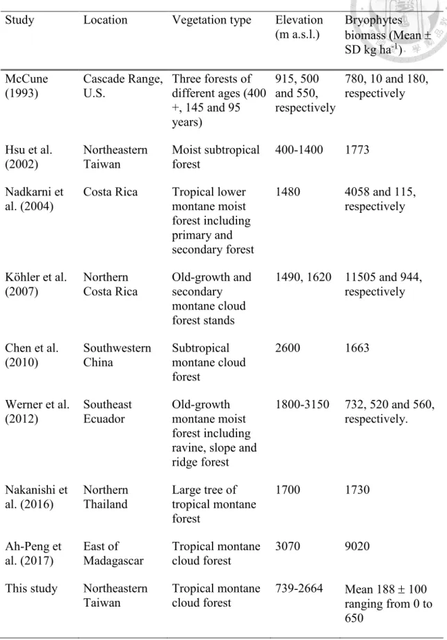
Table 4 Summary of relevant bryophytes biomass research.

Study Location Vegetation type Elevation (m a.s.l.)

Bryophytes biomass (Mean SD kg ha^-1) McCune

(1993) Cascade Range,

U.S. Three forests of different ages (400 +, 145 and 95 years)

915, 500 and 550, respectively

780, 10 and 180, respectively

Hsu et al.

(2002)

Northeastern Taiwan

Moist subtropical forest

400-1400 1773

Nadkarni et al. (2004)

Costa Rica Tropical lower montane moist forest including primary and secondary forest

1480 4058 and 115, respectively

Köhler et al.

(2007)

Northern Costa Rica

Old-growth and secondary montane cloud forest stands

1490, 1620 11505 and 944, respectively

Chen et al.

(2010)

Southwestern China

Subtropical montane cloud forest

2600 1663

Werner et al.

(2012)

Southeast Ecuador

Old-growth montane moist forest including ravine, slope and ridge forest

1800-3150 732, 520 and 560, respectively.

Nakanishi et al. (2016)

Northern Thailand

Large tree of tropical montane forest

1700 1730

Ah-Peng et al. (2017)

East of Madagascar

Tropical montane cloud forest

3070 9020

This study Northeastern

Taiwan Tropical montane

cloud forest 739-2664 Mean 188 100 ranging from 0 to 650

(46)

37

5. Conclusions

To our knowledge, this is the first study to map EB biomass over a vest region in TMCF.

We developed an in-situ general EB depth-biomass allometry and a new non-destructive sampling approach to estimate EB biomass. Combining a previously reported relationship between EB of sampled stem area and an entire tree, we may be able to estimate EB biomass of an entire plot with DBH measures. Based upon statistics and empirical evidences, airborne lidar derived canopy height and digital model may be salient variables to integrate a number of biophysical and topographic attributes for analysis, contributing significantly to our understanding of the salient factors that govern the abundance of EB.

The proposed synoptic sensing approach integrating field measurements of different scales and airborne lidar data may be useful for regional mapping of EB biomass, which might advance our understanding of the role of EB plays in the hydrological cycle of TMCFs.

doi:10.6342/NTU201902408

(47)

Acknowledgments

We appreciate field assistance provided by colleagues and friends especially Ching-Yuan Wang, Hung-Chi Liu, Hsin-Ju Li, Kai-ting Hu, Sheng-Fong Tsai, Zhang Jun. This work was supported by the Ministry of Science and Technology (MOST) (105-2633-M-002- 003-), National Taiwan University and the Research Center for Future Earth and the Ministry of Education of Taiwan (MOE).

(48)

39

Appendix A. Supplementary data

Supplementary data associated with this study was compiled can be found here.

Figure S1 Comparison of model standard residuals. (a) Model 1: W= 10 D^0.83626; (b) Model 2: W=12.61 D^0.722, Model 1 and Model 2 was not calibrated. The standard residuals of epiphytic bryophytes depth at 6 to 8 cm was reduced, while at 0 to 4 cm was larger. (c) Model 3: W=11.96 D^0.753; (d) Model 4: W= 11.78 D ^0.767. Model 3 and Model 4 was calibrated by the variogram of power and exponent respectively.

doi:10.6342/NTU201902408

(49)

Figure S2 Person coefficient correlation matrix for 46 variables

(50)

41

Figure S3 Number of components and root mean square error of prediction (RMSEP) of partial least squares regression. The first fourth components were selected for regional EB estimation (RMSEP = 80.7 kg ha^-1). The RMSEPs were ranging from 102.8 to 78.1 kg ha^-1

doi:10.6342/NTU201902408

(51)

(52)

43

doi:10.6342/NTU201902408

(53)

Figure S4 Epiphytic bryophytes biomass distribution of in eight direction within 21 plots.

(54)

45

doi:10.6342/NTU201902408

(55)

Figure S5 Tree size distribution of twenty-one field plots (Figure 1) with DBH larger than 5 cm (the x-axis).

(56)

47

Reference

Abdi, H. (2003). Partial least square regression (PLS regression). Encyclopedia for research methods for the social sciences, 6(4), 792-795.

Ah-Peng, C., Cardoso, A. W., Flores, O., West, A., Wilding, N., Strasberg, D., &

Hedderson, T. A. J. (2017). The role of epiphytic bryophytes in interception, storage, and the regulated release of atmospheric moisture in a tropical montane cloud forest. Journal of Hydrology, 548, 665-673.

Asner, G. P., Powell, G. V., Mascaro, J., Knapp, D. E., Clark, J. K., Jacobson, J., . . . Victoria, E. (2010). High-resolution forest carbon stocks and emissions in the Amazon. Proceedings of the national academy of sciences, 107(38), 16738- 16742.

Barker, M. G., & Pinard, M. A. (2001). Forest canopy research: sampling problems, and some solutions Tropical Forest Canopies: Ecology and Management (Vol. 153, pp. 23-38). Plant Ecology: Springer.

Barkman, J. J. (1958). Phytosociology and ecology of cryptogamic epiphytes.

Benzing, D. H. (1998). Vulnerabilities of tropical forests to climate change: the significance of resident epiphytes Potential impacts of climate change on tropical forest ecosystems (pp. 379-400): Springer.

Błaś, M., Sobik, M., Quiel, F., & Netzel, P. (2002). Temporal and spatial variations of fog in the Western Sudety Mts., Poland. Atmospheric Research, 64(1-4), 19-28.

Bonan, G. B. (2008). Forests and climate change: forcings, feedbacks, and the climate benefits of forests. science, 320(5882), 1444-1449.

Bonham, C. D. (2013). Measurements for terrestrial vegetation: John Wiley & Sons.

Bruijnzeel, L., Mulligan, M., & Scatena, F. N. (2011a). Hydrometeorology of tropical montane cloud forests: emerging patterns. Hydrological Processes, 25(3), 465- 498.

Bruijnzeel, L. A., Scatena, F. N., & Hamilton, L. S. (2011b). Tropical montane cloud forests: science for conservation and management: Cambridge University Press.

Bubb, P., May, I. A., Miles, L., & Sayer, J. (2004). Cloud forest agenda.

Chang, S.-C., Lai, I.-L., & Wu, J.-T. (2002). Estimation of fog deposition on epiphytic bryophytes in a subtropical montane forest ecosystem in northeastern Taiwan.

Atmospheric Research, 64(1), 159-167.

Chen, L., Liu, W.-y., & Wang, G.-s. (2010). Estimation of epiphytic biomass and nutrient pools in the subtropical montane cloud forest in the Ailao Mountains, south-western China. Ecological research, 25(2), 315-325.

Crowther, T. W., Glick, H. B., Covey, K. R., Bettigole, C., Maynard, D. S., Thomas, S.

M., . . . Amatulli, G. (2015). Mapping tree density at a global scale. Nature, 525(7568), 201.

DeFries, R. (2008). Terrestrial vegetation in the coupled human-earth system:

contributions of remote sensing. Annual Review of Environment and Resources, 33, 369-390.

Deng, Z.-H. (2006). The composition, distribution, and biomass of epiphytic bryophytes of a naturally regenerated Chamaecyparis obtusa var. formosana forest.

(Master Thesis), National Donghua University.

doi:10.6342/NTU201902408

(57)

Dubayah, R., Goetz, S., Blair, J., Fatoyinbo, T., Hansen, M., Healey, S., . . . Luthcke, S.

(2014). The global ecosystem dynamics investigation. Paper presented at the AGU Fall Meeting Abstracts.

Duh, C.-T., Chiu, C.-M., & Lin, K.-C. (2011). Estimate of Above-And Below-Ground Biomass of a Cryptomeria Japonica Plantation in Renluen Area of Taiwan.

Quarterly Journal of Chinese Forestry, 44(3), 401-411.

Enquist, B. J., Brown, J. H., & West, G. B. (1998). Allometric scaling of plant energetics and population density. Nature, 395(6698), 163.

Enquist, B. J., West, G. B., Charnov, E. L., & Brown, J. H. (1999). Allometric scaling of production and life-history variation in vascular plants. Nature, 401(6756), 907.

Fenton, N. J., Frego, K. A., & Sims, M. R. (2003). Changes in forest floor bryophyte (moss and liverwort) communities 4 years after forest harvest. Canadian journal of botany, 81(7), 714-731.

Foster, P. (2001). The potential negative impacts of global climate change on tropical montane cloud forests. Earth-Science Reviews, 55(1-2), 73-106.

doi:10.1016/s0012-8252(01)00056-3

Freiberg, M., & Freiberg, E. (2000). Epiphyte diversity and biomass in the canopy of lowland and montane forests in Ecuador. Journal of Tropical Ecology, 16(5), 673-688.

Gradstein, S. R. (2008). Epiphytes of tropical montane forests—impact of deforestation and climate change. Göttingen Centre for Biodiversity and Ecology. Biodiversity and Ecology Series, 2, 51-65.

Haugerud, R. A., Harding, D. J., Johnson, S. Y., Harless, J. L., Weaver, C. S., &

Sherrod, B. L. (2003). High-resolution lidar topography of the Puget Lowland, Washington. GSA Today, 13(6), 4-10.

Hofstede, R. G., Wolf, J. H., & Benzing, D. H. (1993). Epiphytic biomass and nutrient status of a Colombian upper montane rain forest. Selbyana, 37-45.

Holwerda, F., Bruijnzeel, L., Muñoz-Villers, L., Equihua, M., & Asbjornsen, H. (2010).

Rainfall and cloud water interception in mature and secondary lower montane cloud forests of central Veracruz, Mexico. Journal of Hydrology, 384(1-2), 84- 96.

Hou, C.-S., L.-Y., F., C. -L., C., H.-J., C., Y.-C., H., Hu, J.-C., & C.-W., L. (2014).

Airborne LiDAR DEM and Geohazards Applications. Journal of Photogrammetry and Remote Sensing, 18(2), 93–108.

Houghton, R. (2005). Aboveground forest biomass and the global carbon balance.

Global Change Biology, 11(6), 945-958.

Hsu, C.-C., Horng, F.-W., & Kuo, C.-M. (2002). Epiphyte biomass and nutrient capital of a moist subtropical forest in north-eastern Taiwan. Journal of Tropical Ecology, 18(5), 659-670.

Huang, C.-M., Duh C. -T, C., & S. -C, L., K. -C. (2012). Estimation of tree biomass and growth of Hiniji stand in Chilanshan area of North-eastern Taiwan. Quarterly Journal of Chinese Forestry, 45(2), 137-150.

Jucker, T., Hardwick, S. R., Both, S., Elias, D. M., Ewers, R. M., Milodowski, D.

T., . . . Coomes, D. A. (2018). Canopy structure and topography jointly constrain the microclimate of human‐modified tropical landscapes. Global Change

Biology, 24(11), 5243-5258.

(58)

49

Köhler, L., Tobón, C., Frumau, K. A., & Bruijnzeel, L. S. (2007). Biomass and water storage dynamics of epiphytes in old-growth and secondary montane cloud forest stands in Costa Rica. Plant ecology, 193(2), 171-184.

Kleiber, M. (1947). Body size and metabolic rate. Physiological reviews, 27(4), 511- 541.

Lai, I.-L., Chang, S.-C., Lin, P.-H., Chou, C.-H., & Wu, J.-T. (2006). Climatic characteristics of the subtropical mountainous cloud forest at the Yuanyang Lake long-term ecological research site, Taiwan. Taiwania, 51(4), 317-329.

Lefsky, M. A., Cohen, W., Acker, S., Parker, G. G., Spies, T., & Harding, D. (1999).

Lidar remote sensing of the canopy structure and biophysical properties of Douglas-fir western hemlock forests. Remote sensing of environment, 70(3), 339-361.

Lefsky, M. A., Cohen, W. B., Parker, G. G., & Harding, D. J. (2002). Lidar remote sensing for ecosystem studies: Lidar, an emerging remote sensing technology that directly measures the three-dimensional distribution of plant canopies, can accurately estimate vegetation structural attributes and should be of particular interest to forest, landscape, and global ecologists. BioScience, 52(1), 19-30.

Lefsky, M. A., Harding, D. J., Keller, M., Cohen, W. B., Carabajal, C. C., Del Bom Espirito‐Santo, F., . . . de Oliveira Jr, R. (2005). Estimates of forest canopy height and aboveground biomass using ICESat. Geophysical research letters, 32(22).

Ligrone, R., Duckett, J., & Renzaglia, K. (2000). Conducting tissues and phyletic relationships of bryophytes. Philosophical Transactions of the Royal Society of London. Series B: Biological Sciences, 355(1398), 795-813.

Luna-Vega, I., Morrone, J. J., Ayala, O. A., & Organista, D. E. (2001). Biogeographical affinities among Neotropical cloud forests. Plant Systematics and Evolution, 228(3-4), 229-239.

McCune, B. (1993). Gradients in epiphyte biomass in three Pseudotsuga-Tsuga forests of different ages in western Oregon and Washington. Bryologist, 405-411.

McCune, B., Amsberry, K., Camacho, F., Clery, S., Cole, C., Emerson, C., . . . Harris, R. (1997). Vertical profile of epiphytes in a Pacific Northwest old-growth forest.

Northwest Science, 71(2), 145-152.

McCune, B., Rosentreter, R., Ponzetti, J. M., & Shaw, D. C. (2000). Epiphyte habitats in an old conifer forest in western Washington, USA. The Bryologist, 103(3), 417-427.

Mevik, B.-H., & Wehrens, R. (2015). Introduction to the pls Package. Help Section of The “pls” package of RStudio Software, 1-23.

Moffett, M. W., & Lowman, M. D. (1995). Canopy access techniques. Forest canopies, 3-26.

Moore, I. D., Grayson, R., & Ladson, A. (1991). Digital terrain modelling: a review of hydrological, geomorphological, and biological applications. Hydrological Processes, 5(1), 3-30.

Nöske, N. M., Hilt, N., Werner, F. A., Brehm, G., Fiedler, K., Sipman, H. J., &

Gradstein, S. R. (2008). Disturbance effects on diversity of epiphytes and moths in a montane forest in Ecuador. Basic and Applied Ecology, 9(1), 4-12.

Nadkarni, N. M., Schaefer, D., Matelson, T. J., & Solano, R. (2004). Biomass and nutrient pools of canopy and terrestrial components in a primary and a

doi:10.6342/NTU201902408