行政院國家科學委員會專題研究計畫 成果報告
利用 SDRE 方法之微衛星姿態與位置最佳軌跡規劃研究 研究成果報告(精簡版)
計 畫 類 別 : 個別型
計 畫 編 號 : NSC 100-2221-E-011-061-
執 行 期 間 : 100 年 08 月 01 日至 101 年 07 月 31 日 執 行 單 位 : 國立臺灣科技大學自動化及控制研究所
計 畫 主 持 人 : 郭永麟
計畫參與人員: 碩士班研究生-兼任助理人員:劉世民 碩士班研究生-兼任助理人員:林子鑌
公 開 資 訊 : 本計畫可公開查詢
中 華 民 國 101 年 09 月 20 日
中 文 摘 要 : 本研究報告探討兩種以 SDRE 為基礎的積分式滑動模式控制 (sliding mode control, ISM)法則,而且將它們應用於人造 衛星姿態動力之混沌系統。SDRE 為 state-dependent
Riccait Equation (狀態相依之瑞卡提方程式)之縮寫,它具 有非線性系統之控制器設計的彈性,而積分式滑動模式控制 可以消除穩態誤差,未了得到兩種方法的優點,在本研究中 針對非線性系統提出兩個整合方法,且被稱做 SDRE-ISM 和 ISM-SDRE。數值範例顯示了 SDRE-ISM 可提供較小的性能指標 (performance index)值,而 ISM-SDRE 可提供較小的時間達 到穩態,此外當有亂數雜訊影響到系統時,以 ISM 為基礎的 方法可降低穩態誤差。
中文關鍵詞: 狀態相依之瑞卡提方程式、積分式滑動模式控制、人造衛星 姿態動力之混沌系統
英 文 摘 要 : This report investigates two SDRE-based integral sliding mode (ISM) controls, and they are applied to a chaotic spacecraft attitude dynamic system. The SDRE method is short for the State-Dependent Riccati Equation method, and it has the design flexibility for nonlinear control. The ISM control can eliminate the steady-state error. To gain the advantages of both methods, their combination methods, called SDRE- ISM and ISM-SDRE in this paper, are generalized for nonlinear systems. The numerical examples show that the SDRE-ISM method provides the smallest value of the performance index, and the ISM-SDRE provides the minimum time to reach the steady state. Besides, the ISM-based method can have the smaller steady-state errors when a random disturbance is included to the system.
英文關鍵詞: state-dependent Riccati equation (SDRE), integral sliding mode control, chaotic spacecraft attitude dynamic system
□期中進度報告 行政院國家科學委員會補助專題研究計畫
▉期末報告
利用 SDRE 方法之微衛星姿態與位置最佳軌跡規劃研究
計畫類別:▉個別型計畫 □整合型計畫
計畫編號:NSC 100 - 2221 - E - 011 - 061 - 執行期間: 100 年 8 月 1 日至 101 年 7 月 31 日 執行機構及系所:國立臺灣科技大學 自動化及控制研究所
計畫主持人:郭永麟 共同主持人:
計畫參與人員:劉世民、林子鑌
本計畫除繳交成果報告外,另含下列出國報告,共 0 份:
□移地研究心得報告
□出席國際學術會議心得報告
□國際合作研究計畫國外研究報告
處理方式:除列管計畫及下列情形者外,得立即公開查詢
□涉及專利或其他智慧財產權,□一年▉二年後可公開查詢 中 華 民 國 101 年 9 月 20 日
中文摘要
本研究報告探討兩種以 SDRE 為基礎的積分式滑動模式控制(sliding mode control, ISM)法則,而且將它們應用於人造衛星姿態動力之混沌系統。SDRE 為 state-dependent Riccait Equation (狀態相依之瑞卡提方程式)之縮寫,它具有非線性 系統之控制器設計的彈性,而積分式滑動模式控制可以消除穩態誤差,未了得到 兩種方法的優點,在本研究中針對非線性系統提出兩個整合方法,且被稱做 SDRE-ISM 和 ISM-SDRE。數值範例顯示了 SDRE-ISM 可提供較小的性能指標 (performance index)值,而 ISM-SDRE 可提供較小的時間達到穩態,此外當有亂 數雜訊影響到系統時,以 ISM 為基礎的方法可降低穩態誤差。
關鍵字:狀態相依之瑞卡提方程式、積分式滑動模式控制、人造衛星姿態動力之 混沌系統
Abstract
This report investigates two SDRE-based integral sliding mode (ISM) controls, and they are applied to a chaotic spacecraft attitude dynamic system. The SDRE method is short for the State-Dependent Riccati Equation method, and it has the design flexibility for nonlinear control. The ISM control can eliminate the steady-state error. To gain the advantages of both methods, their combination methods, called SDRE-ISM and ISM-SDRE in this paper, are generalized for nonlinear systems. The numerical examples show that the SDRE-ISM method provides the smallest value of the performance index, and the ISM-SDRE provides the minimum time to reach the steady state. Besides, the ISM-based method can have the smaller steady-state errors when a random disturbance is included to the system.
Keywords: state-dependent Riccati equation (SDRE), integral sliding mode control, chaotic spacecraft attitude dynamic system
Acknowledgements
The study was sponsored with a grant, NSC-100-2221-E-011-061, from National Science Council, Taiwan.
Contents
中文摘要 ... I Abstract...II Acknowledgements ... III Contents ... IV
1. Introduction ... 1
2. Chaotic attitude dynamics of spacecraft ... 2
3. SDRE-based integral sliding mode (ISM) control ... 4
3.1. SDRE control... 4
3.2. ISM control... 5
3.3. ISM-SDRE control... 5
3.4. SDRE-ISM control... 7
4. Numerical simulations ... 8
5. Conclusions ...13
References...14
附件一:國科會補助專題研究計畫成果報告自評表 ...16
附件二: 論文發表情形 ...17
1. Introduction
Chaotic phenomena widely exist in physical systems such as lasers, oscillators, radars, etc., and there are numerous approaches developed to deal with the control of chaotic systems. Ott, Grebogi, and Yorke proposed a feedback chaos control techniques, which is called the OGY approach and is based on the fact that there is an infinite number of unstable periodic orbits embedded within a chaotic attractor [1].
After that, Numerous amounts of the researches applied various nonlinear control methods, such as feedback linearization, sliding-mode approach, Lyapunov-based control technique, LMI based nonlinear technique, nonlinear H, linear time-delay feedback control, to the control of chaotic systems [2-6]. For spacecraft attitude dynamics, its chaotic behavior exists in some models of spacecraft such as spinning satellites in a circular orbit, gyrostat satellites in the gravitational field, and tethered satellites. Thus, a considerable amount of effort was devoted to chaotic attitude control during the past few decades. Kong et al. investigated the dynamics of spacecraft attitude motion, and a controller with position and velocities feedback was utilized to suppress the chaos and control system to the given fixed point and periodic orbit [7]. Kemih et al. applied impulsive control to a six-dimensional system which describes the attitude dynamics of a satellite subjected to deterministic external perturbations which induce chaotic motion when no control is affected [8]. Inarrea studied the pitch motion of an asymmetric magnetic spacecraft influenced by a gravity gradient torque, and a linear time-delay feedback method was applied to remove the chaotic character of initially irregular attitude motions [9]. Sadaoui et al. presented a systematic design procedure to synchronize two identical chaotic satellites systems based on a predictive control [10]. Mohammadbagheri et al. proposed the model predictive control method to stabilize the Lorenz-type chaotic attitude of a satellite and to suppress the chaos and regulate the state trajectory of this system [11].
The main advantage of the sliding mode control (SMC) is effectively to compensate the errors due to external disturbances. Young et al. studied the sliding surface design by using the LQR approach [12], and Utkin investigated the optimal sliding surface design of time-varying systems [13]. After that, there are numerous researchers devoted to this field. For linear systems, Xu et al. studied the optimal SMC for linear systems by combining the LQR and the integral sliding mode (ISM) control [14]. Dong et al. designed an optimal sliding surface based on the successive approximation approach for linear time-delay systems [15]. Pang et al. designed optimal sliding mode output tracking controllers for uncertain linear systems with the reference signals given by exosystem outputs [16]. For nonlinear systems, the State-Dependent Riccati Equation (SDRE) strategy, first proposed by Pearson [17], can be incorporated. The method expresses a nonlinear state equation as a linear-like
state equation, where the coefficient matrices are functions of the states. Thus, a linear quadratic regulator (LQR) problem can be formulated, and a sub-optimal solution is found by solving an algebraic state-dependent Riccati equation. Salamci et al.
designed a controller based on the SMC and SDRE for a nonlinear missile system, which tracks a given acceleration command [18]. Pukdeboon et al. studid optimal sliding mode control laws using the ISM for some spacecraft attitude tracking problems [19]. Ikeda proposed an active steering method using adaptive sliding mode control based on the SDRE for the four-wheel-steering vehicle [20].
The SDRE has the design flexibility for nonlinear control, and the ISM can eliminate the steady state error. To gain the advantages of both methods, a limited number of papers were ever integrated them, but they were not generalized for all nonlinear systems. Besides, the integrated methods have not applied to chaotic systems. This paper first briefly introduced the SDRE and ISM methods, and then two integrated methods are presented, which are the SDRE-based ISM methods. There are total four control methods applied to a chaotic attitude dynamics of spacecraft, and their control performances are compared This paper is organized as follows. Section 2 presents the chaotic attitude dynamics of spacecraft. Section 3 presents the SDRE, ISM, SDRE-ISM, and ISM-SDRE controls. The last two controls are the integrated methods. Section 4 demonstrates numerical simulations, and Section 5 concludes significant results.
2. Chaotic attitude dynamics of spacecraft
The attitude of spacecraft is expressed as a set of 3-2-1 Euler angles (,,), and then the spacecraft attitude kinematics equations are given as
z y x
sec cos sec
sin 0
sin cos
0
tan cos tan
sin 1
(1)
where , x and y are angular velocities along the x-, y- and z-axes fixed on z the space, respectively.
Based on Euler equations, the attitude dynamics of spacecraft can be written as
z z y x y x z z
y y x z x z y y
x x z y z y x x
C D I
I I
C D I
I I
C D I
I I
) (
) (
) (
(2)
where I , x Iy and I are the moments of inertia; z D , x Dy and D are the z
disturbance torques; C , x Cy and C are the control torques. z
To demonstrate the chaotic attitude motion of spacecraft, Reference [21]
considered the disturbance torques as
sin cos
sin cos
sin cos 4
. 0 0
6
0 35 . 0 0
2 / 6 0 2 . 1
z y x
z y x
D D D
(N-m) (3)
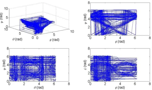
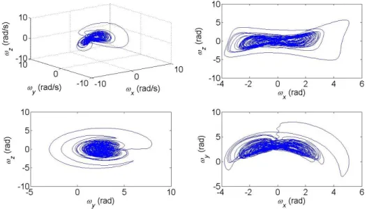
Besides, there is no control torques applied to the attitude system, and the moments of inertia are (Ix,Iy,Iz)(3,2,1) kg-m2. Figs. 1-2 show the phase portraits of the chaotic attitude motion with the initial conditions (,,)(0,0,0) and
) 3 , 1 . 4 , 2 ( ) , ,
(x y z rad/sec. In this system, the Lyapunov exponents are given as [21]
( , , , x, y, z)(0.3629, 0.1313, 0.0174, 0.0077, 0.0721, 0.7509)
Therefore, the system is chaotic because the Lyapunov exponents are both positive and negative.
Fig. 1. Phase portraits of Euler angles
Fig. 2. Phase portrait of angular velocities
3. SDRE-based integral sliding mode (ISM) control
There are four controllers studied in this section. The SDRE control and the ISM control are introduced first, and then two SDRE-based ISM controllers are presented.
The following section will perform the applications of the four controllers, which will show their performance comparisons.
3.1. SDRE control
A nonlinear and observable system is written as )
( ) ( ) ( )
(t f x g x u t
x , x(0)x0 (4)
where x(t) and u(t) are the state and input vectors, respectively.
To perform a regulation problem, an infinite-time performance index is written as
dt t u x R t u t x x Q x x t
u x
J [ T( ) ( ) ( ) T( ) ( ) ( )]
2 )) 1 ( ,
( 0
0 (5)where Q(t)0 and R(t)0 are state-dependent weighting matrices.
To apply the LQR, Eq. (4) can be factorized in a linear-like structure as )
( ) ( ) ( )
(t A x x B x u t
x (6)
where f(x) A(x)x and g(x)B(x). There is an infinite number of forms to factorize f(x) as A )(x x, so this property increases the flexibility of the SDRE.
Solving Eqs. (5) and (6) by following the formulation of the LQR leads to x
x P x B x R x x K t
u( ) ( ) 1( ) T( ) ( ) (7)
where P( x) is the symmetric and positive-definite solution of the algebraic
State-Dependent Riccati Equation as
0 ) ( ) ( ) ( ) ( ) ( ) ( ) ( ) ( ) ( )
(x A x A x P x P x B x R1 x B x P x Q x
P T T (8)
3.2. ISM control
An integral sliding surface is written as )) 0 ( ( )
( ))
( ( )
( 0
0 0
0 x t s dt s x
s t
s
t (9)where s0(x(t)) is a specified sliding surface, and is a parameter. It is obvious that s(0)0.
One defines s 0 Cx, where C is a constant matrix, and differentiating Eq. (9) and substituting into Eq. (4) leads to
)]
( [
)) ( ( )
(t Cg x 1 Cx Cf x
u (10)
A sliding mode control is designed to keep the system on the sliding surface or inside a boundary layer around the sliding surface such that s , where is a positive constant number. Thus, the control in Eq. (10) is rewritten as
) ( )]
( [
)) ( ( )
(t Cg x 1 Cx Cf x M s
u (11)
where M 0 is a constant number such that M d , in which d is a disturbance, and is a positive number; (s) is a saturation function as
1 / 1 )
(
s s ,
s s s
if if if
(12)
A Lyapunov function is defined as 2 0
1
s s
V T (13)
Then, its time derivative is obtained as 0 ) ( )
)(
(
s s sCg x M d Cg x s
V T (14)
where C is designed to satisfy Cg(x)0, and M is chosen such M supd . Thus, based on Eqs. (13) and (14), the control shown in Eq. (11) guarantees that the state asymptotically converges to zero as time goes to infinity.
3.3. ISM-SDRE control
Reference [14] presented an optimal sliding mode control for linear systems.
This section will generalize the approach for nonlinear systems. This generalized approach is to perform the ISM control first, and then the SDRE control is applied to
find the optimal sliding surface. Thus, this generalized approach is called the ISM-SDRE control
A sliding surface is defined as
) 0 ( ) ( ) ( )) 0 ( ( ) ( ) ( )
(t s0 x y t s0 x Cx t y t Cx
s (15)
where
tv dt t
y( ) 0 () (16)
or
) ( ) (t v t
y with y(0)0 (17)
Define a new state vector as t T
y t x t
z( )[ ( ) ( )] (18)
Differentiating Eq. (15) and substituting into Eq. (6) lead to ]
) ( ) ( [ )) ( ( )
(t CB x 1 v t CA x x
u (19)
To keep the system on the sliding surface or inside a boundary layer around the sliding surface, the control is rewritten as
M x x CA t v x CB t
u( )( ( ))1[ ( ) ( ) ] (20)
Since the system will stay inside the boundary layer from s(0)0, the control can be further expressed as
) ( ) ( ) ( ) ( / ] ) ( ) ( [ )) ( ( )
(t CB x 1 v t CA x x Ms a x z t b x v t
u (21)
where
CB CA M M
x
a( ) ( )1 , b(x)(CB)1, M M/ (22) Substituting Eq. (21) into (6) and combining (17) lead to a new set of state equations as
) ( ) ( ) ( ) ( )
(t G z z t H z v t
z (23)
where
0 0
) ( )
( ) ( )) ( )(
( ) ( ) [ (
1
C B x M
M x B x CA x CB x B x z A
G (24)
T T
TB x I
x CB z
H( )[( ( )) ( ) ] (25)
in which I is an identity matrix.
Eq. (23) is transformed from (6) by imposing the sliding surface shown in (15), and v(t) can be treated as an input in (23). Based on Eq. (23), the performance index shown in (6) should be also transformed as
dt t v x N t v t v x H t z t z x M x z t
v x
J [ T( ) ( ) ( ) 2 T( ) ( ) ( ) T( ) ( ) ( )]
2 )) 1 ( ,
( 0
0 (26)where
) ( ) ( ) ( ) ( )
(x T Q x T a x R x a x
M T T (27)
) ( ) ( ) ( )
(x a x R x b x
H T (28)
) ( ) ( ) ( )
(x b x R x b x
N T (29)
in which T is a constant matrix such that x Tz.
The optimal solution regarding to the transformed regulation problem related to (26) and (23) is given as
z x H x S x H x N z z L t
v( ) ( ) ( )1[ ( )T ( ) T( )] (30) where S(x) is the solution of the generalized algebraic state-dependent Riccati equation as
0 ) ( )]
( ) ( ) ( )[
( )]
( ) ( ) ( [ ) ( ) ( ) ( )
( 1
S x G x GT x S x P x B x H x N x HT x S x HT s M x (31) A Lyapunov function is defined and is the same as Eq. (13), and its time derivative is obtained as
0 ) ( )
)(
(
s s sCB x M d CB x s
V T (32)
where C is designed such that CB(x)0 for any instant of time, and M is chosen such M supd . Then, the control shown in Eq. (21) guarantees that the state asymptotically converges to zero as time goes to infinity.
3.4. SDRE-ISM control
To distinguish the SDRE-ISM control from the SDRE-ISM controller presented in the previous subsection, this approach is to find an SDRE solution first and then to perform the ISM method. Reference [19] has presented this approach for the quaternion-based attitude dynamics. This subsection will generalize this approach for general nonlinear systems expressed in Eq. (4).
One performs the SDRE method first, and the optimal solution for Eqs. (5) and (6) is written as
x x P x B x R x x K t
u( ) ( ) 1( ) T( ) ( ) (33)
where P( x) is the solution of the algebraic State-Dependent Riccati Equation as Eq.
(8).
A sliding surface is defined and is the same as Eq. (15). Differentiating Eq. (15) leads to
] ) ( ) ( [ )
(t C f x g x u
y with y(0)Cx(0) (34)
To keep the system on the sliding surface or inside a boundary layer around the sliding surface, the control is modified as
M t u t
u( ) ( ) (35)
A Lyapunov function is defined and is the same as Eq. (13), and its time derivative is the same as (14). Thus, the control shown in Eq. (35) guarantees that the state asymptotically converges to zero as time goes to infinity.
4. Numerical simulations
The four controllers presented in previous section are applied to the chaotic attitude motion of spacecraft mentioned in Section 2, and the system equations Eqs.
(1), (2) and (3) form a set of state equation as )
( ) ( ) ( ) ( ) ( )
(t f x g x u t h x d t
x (36)
where
x y z
Tt
x( ) (37)
z y x y x
y x z z x
x z y z y
z y
z y
z y
x
I I I
I I I
I I x I
f
/ ) (
/ ) (
/ ) (
sec cos sec
sin
sin cos
tan cos tan
sin
) (
(38)
Ix Iy Iz
TX h x
g( ) ( ) 0 0 0 1/ 1/ 1/ (39)
sin cos 4
. 0 6
sin cos 35
. 0
sin cos )
2 / 6 ( 12 0 0 0
) (
s x
d
z x
y
z x
(40)
For the SDRE method, implementation of the four controllers, the nonlinear function is factorized as f(x) A(x)x, where
3 3
3 3
1 sin tan cos tan
0 0 cos sin
0 sin sec cos sec
( ) 0 ( ) / 0
0 0 0 ( ) /
( ) / 0 0
z y z x
x z x y
y x y z
A x I I I
I I I
I I I
(41)
Besides, the weighting matrices are selected as Q 100 diag(1,1,1,1,1, ) and R 1. For the ISM method, the parameters of the siding surface
) 0 ( )
(t Cx 0Cxdt Cx
s
t are selected C
I33 I33
and 1 . And, thematrix CB x ( ) diag(1/ 3,1 / 2,1) , which implies that the states converge to zeros, 0 according to the derivation of the control law shown in previous section. Furthermore, the parameters of the controllers are selected as M 10 and 0.1
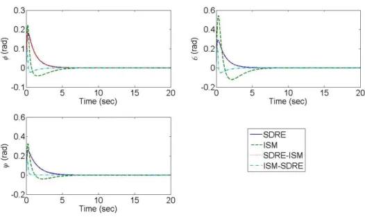
Figs. 3-5 show the time response of the Euler angles, the angular velocities, and the control signals for the chaotic attitude control. The results show that all controllers can drive the states back to zeros. Table 1 shows the performance comparisons of the four controls for the chaotic attitude control. The results show that the ISM-SDRE control has the smallest norm of the states, but it has the largest norm of the control signals. Also, the SDRE-ISM has the smallest performance index. Examining the time to reach the steady state, the ISM-SDRE provides the minimal time. (One requires that the norm of the states should be less than 0.001.)
Fig. 3. Times responses of Euler angles for chaotic attitude control
Fig. 4. Time response of angular velocities for chaotic attitude control
Fig. 5. Time responses of control signals for chaotic attitude control Table 1. Performance comparisons for chaotic attitude control Controllers Norm of
states x
Norm of control signals C
Performance index J
Time to steady state* t ss
SDRE 1.2041 26.9873 4.3665e+2 7.5152
ISM 1.7257 25.3189 4.6942e+2 9.3873
SDRE-ISM 1.2178 26.9301 4.3483e+2 7.4673
ISM-SDRE 1.1723 43.7666 1.0265e+3 6.4409
*The time to reach the steady state satisfies x 103.
The numerical simulations are performed with the initial conditions as
) 2 . 0 , 2 . 0 , 2 . 0 ( ) , ,
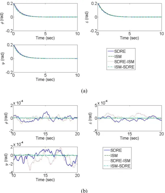
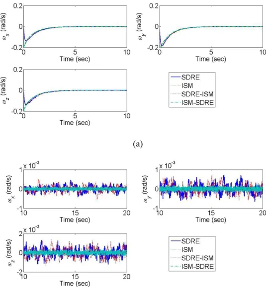
( rads and (x,y,z)(0,0,0) rad/sec. Besides, in order to show the capabilities of the ISM control, the Gaussian random noises with zero mean and a standard deviation set to 1 are considered as the disturbance torques. Figs. 6-8 show the time response of the Euler angles, the angular velocities, and the control signals for the attitude control with the random disturbance torques. The results show that all controllers can drive the states back to zeros. Examining the steady state in the figures, the ISM and ISM-SDRE controls provides smaller variations of the Euler angles and the angular velocities to compare with the SDRE and SDRE-ISM controls.
However, the ISM and ISM-SDRE controls generate larger control signals at the steady state. These results can be also examined from Table 2.
(a)
(b)
Fig. 6. Times responses of Euler angles for attitude control with random disturbance torques (a) from 0 to 10 sec. (b) from 10 to 20 sec.
(a)
(b)
Fig. 7. Time response of angular velocities for attitude control with random disturbance torques (a) from 0 to 10 sec. (b) from 10 to 20 sec.
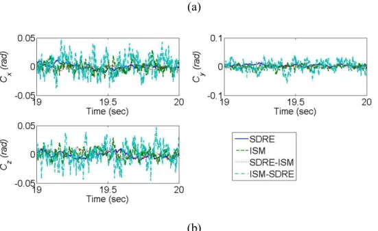
(a)
(b)
Fig. 8. Time responses of control signals for attitude control with random disturbance torques (a) from 0 to 1 sec. (b) from 19 to 20 sec.
Table 2. Performance comparisons at steady state for attitude control with random disturbance torques
Controllers Maximum Euler angle (rad)
Maximum angular velocity (rad/s)
Maximum control signal (N-m)
SDRE 2.019e-4 1.574e-3 2.389e-2
ISM 2.456e-5 3.711e-4 5.007e-2
SDRE-ISM 2.974e-4 1.614e-3 2.525e-2
ISM-SDRE 1.776e-5 5.905e-4 9.516e-2
5. Conclusions
This paper presents four types of controllers, which are the SDRE, ISM, SDRE-ISM, and ISM-SDRE methods, and they are applied to the chaotic attitude motion of spacecraft. The SDRE can be treated as a modified LQR method, because a nonlinear system is factorized as state-space equations with a linear-like structure.
Thus, a Riccatti equation becomes a state-dependent equation, and this provides a suboptimal solution. The ISM method is broadly applied to nonlinear systems with disturbances, and it can reduce steady-state errors. To gain the advantages of the SDRE and ISM, this paper first briefly introduces them, and then two controllers based on their combinations are presented, which are the SDRE-ISM and ISM-SDRE methods. The difference of the two methods is the order of applying both methods.
The numerical examples demonstrate that the SDRE-ISM method provides the smallest value of the performance index, and the ISM-SDRE provides the minimum time to reach the steady state. For the system with the random disturbance torques, the ISM and ISM-SDRE can have the smaller steady-state Euler angles and angular
velocities.
References
[1] E. Ott, C. Grebogi, and J. A. Yorke, Controlling chaos, Phys. Rev. Lett. 64, 1196-1199, 1990.
[2] H. T. Yu, Y. K. Wong, W. L. Chan, K. M. Tsang, and J. Wang, Feedback linearization control of chaos synchronization in coupled map-based neurons under external electrical stimulation, International Journal of Control, Automation and Systems, Vol. 9, No., 5, pp. 867-874, 2011.
[3] C. C. Wang, N. S. Pai, H. T. Yau, Chaos control in AFM system using sliding mode control by backstepping design, Communications in Nonlinear Science and Numerical Simulation, Vol. 15, No. 3, pp. 741-751, 2010.
[4] H. Nijmeijer and H. Berghuis, On Lyapunov Control of the Duffing Equation, IEEE Transactions on Circuits and Systems – I: Fundamental Theory and Applications, Vol. 42, No. 8, pp. 473-477, 1995.
[5] S. Kuntanapreeda, Chaos synchronization of unified chaotic systems via LMI, Physics Letters A, Vol. 373, No. 32, pp. 2837-2840, 2009.
[6] C. K. Ahn, B. K. Kwon, Bo Kyu and Y. S. Lee, Adaptive H synchronization for chaotic systems with unknown parameters and time-delay, Advanced Science Letters, Vol. 3, No. 4, pp. 531-536, 2010.
[7] L. Y. Kong, F. Q. Zhou and J. Zou, The control of chaotic attitude motion of a perturbed spacecraft, the Proceedings of the 25th Chinese Control Conference, Harbin, China, pp. 166-170, 2006.
[8] K. Kemih, A. Kemiha and M. Ghanes, Chaotic attitude control of satellite using impulsive control, Chaos, Solitons and Fractals, Vol. 42, 735-744, 2009.
[9] M. Inarrea, Chaos and its control in the pitch motion of an asymmetric magnetic spacecraft in polar elliptic orbit, Chaos, Solitons and Fractals, Vol. 40, pp.
1637-1652, 2009.
[10] D. Sadaoui, A. Boukabou, N. Merabtine, and M. Benslama, Predictive synchronization of chaotic satellites systems, Expert Systems with Applications Vol. 38, pp. 9041-9045, 2011.
[11] A. Mohammadbagheri and M. Yaghoobi, Lorenz-type chaotic attitude control of satellite through predictive control, the Proceedings of the third International Conference on Computational Intelligence, Modeling and Simulation, Langkawi, Malaysia, pp. 147-152, 2011.
[12] K. K. Young, P. Kokotovic and V. Utkin, A singular perturbation analysis of high-gain feedback systems, IEEE Transactions on Automatic Control, Vol. 22, No. 6 pp. 931-938, 1977.