JOURNAL OF COMPUTING IN CIVIL ENGINEERING / JANUARY 1999 / 1
MS
㛭CMAC N
EURAL
N
ETWORK
L
EARNING
M
ODEL IN
S
TRUCTURAL
E
NGINEERING
By Shih-Lin Hung
1and J. C. Jan
2ABSTRACT: The present American Institute of Steel Construction specifications use the alignment charts and approximate formulas conveniently to determine some coefficients in design, such as moment gradient coefficient Cb for beams of I-shaped section and effective length factor K of columns. In these methods, the coefficients are unconservative when the boundary conditions are different from the development of specifications. The governing equations, numerical approaches, on the K and Cb coefficients provide more accurate results. The approaches, however, are not readily available for structural engineers to use in design. Applying neural network computing toward structural engineering problems has received increasing interest, with particular emphasis placed on supervised neural networks. The cerebellar model articulation controller (CMAC), one of the super-vised neural network learning models, is mostly used in the domain of control. In this work, we use a newly developed Macro Structure CMAC (MS㛭CMAC) neural network learning model to aid steel structure design. The topology of the novel learning model is constructed by a number of time inversion CMACs as a tree structure. The learning performance of the MS㛭CMAC is first compared with a stand-alone time inversion CMAC using one structural engineering example. That comparison indicates not only superior prediction but also fast learning propriety for the MS㛭CMAC neural network learning model. In addition, the MS㛭CMAC neural network learning model is applied to two steel design problems. It is shown that the MS㛭CMAC not only can learn structural design problems within a reasonable central processing unit time but also can estimate more accurate coefficients than that estimated through alignment charts and approximate formulas in American Institute of Steel Construction specifications.
INTRODUCTION
Learning is one of the important features of artificial neural networks. Several neural networks learning algorithms have been developed and explored in a number of different do-mains. In the application of structural engineering, most re-search works were based on the supervised back-propagation neural network (BPN) (Rumelhart et al. 1986) due to its sim-plicity. Vanluchene and Sun (1990) presented a research using the back-propagation learning algorithm in structural design problems. Several other researches, based on BPN learning algorithm, have applied neural network computing models in structural engineering and related engineering problems [Gha-boussi et al. (1991), Hajela and Berke (1991), Elkordy et al. (1994), Goh (1995), Kasperkiewicz et al. (1995), Mukherjee and Desphande (1995), and others].
BPN learning models, however, always take a long time in learning process. Several approaches for improving the learn-ing performance of a BPN learnlearn-ing algorithm have been achieved and reported in recent literature. One approach is to develop more effective learning algorithms with the objective of reducing the learning time. For instance, Adeli and Hung (1994) developed an adaptive conjugate gradient neural net-work (Ad-CGN) learning algorithm and applied it to structural engineering. Based on a limited memory BFGS quasi-Newton second-order method (Nocedal 1990), a more effective adap-tive L-BFGS learning algorithm was developed by Hung and Lin (1994). Another approach is to develop a parallel algo-rithm on multiprocesser computers with the objective of re-ducing the overall computing time. For instance, Adeli and Hung (1993) presented a concurrent Ad-CGN learning algo-rithm to a large-scale pattern recognition problem. Significant
1
Assoc. Prof., Dept. of Civ. Engrg., Nat. Chiao Tung Univ., 1001 Ta Hsueh Rd., Hsinchu Taiwan 300, R.O.C.
2PhD Candidate, Dept. of Civ. Engrg., Nat. Chiao Tung Univ., 1001
Ta Hsueh Rd., Hsinchu Taiwan 300, R.O.C.
Note. Discussion open until June 1, 1999. To extend the closing date one month, a written request must be filed with the ASCE Manager of Journals. The manuscript for this paper was submitted for review and possible publication on March 6, 1998. This paper is part of the Journal
of Computing in Civil Engineering, Vol. 13, No. 1, January, 1999.
䉷ASCE, ISSN 0877-3801/99/0001-0001–0011/$8.00 ⫹ $.50 per page.
Paper No. 17857.
improvement for the BPN algorithm in computing time was reported in their work. The third approach is the development of hybrid neural network learning algorithms. Hung and Adeli (1994) presented a parallel hybrid genetic/neural network learning algorithm, integrating a genetic algorithm with the Ad-CGN learning algorithm, in engineering and pattern rec-ognition problems. They reported a superior convergence property of the parallel hybrid neural network learning algo-rithm as compared with a BPN learning algoalgo-rithm. Further-more, Gunaratnam and Gero (1994) discussed the effect of representation of input/output pairs for training instances on the learning performance of the BPN learning algorithm in the problems of structural design.
Unsupervised learning models are the other major neural network learning techniques and have been applied to several domains, mostly in the problems of classification. In structural engineering problems, Adeli and Park (1995) compared the learning performance of counterpropagation neural networks (CPN) and BPN. The CPN learning model is a combination of supervised and unsupervised mapping neural network learn-ing models. Kasperkiewicz et al. (1995) used a fuzzy neural network to predict the strength of high performance concrete. The fuzzy neural network, called fuzzy-ARTMAP, is a map-ping neural network of combining Kohonen learning and Grossberg learning algorithms (Hecht-Nielsen 1987). Re-cently, Hung and Jan (1997) presented an integrated fuzzy neural network learning model by integrating a novel unsu-pervised fuzzy neural network reasoning model with a super-vised learning model in the domain of structural engineering. The unsupervised fuzzy neural network reasoning model was developed on the basis of a single-layer laterally connected neural network with an unsupervised competing algorithm. The integrated fuzzy neural network learning model demon-strated its superior learning performance in complicated struc-tural design problems with a reasonable computational time.
A cerebellar model articulation controller (CMAC) neural network, one of the supervised neural networks learning mod-els, is mostly used in the domain of control. The merits of a CMAC neural network are not only its fast convergence in the learning phase but also its capability of mapping complicated nonlinear functions (Albus 1975a). However, the performance of a well-trained CMAC neural network in verification phases
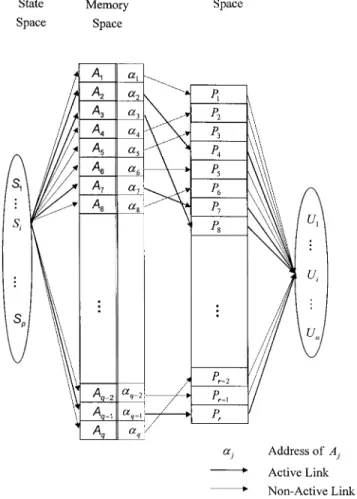
FIG. 1. Simple CMAC Neural Network in Four Spaces with Three Corresponding Mappings
is extremely dependent upon some predefined working param-eters, such as the size of association memory and physical memory used. To improve the performance of CMAC neural network learning models, Albus (1975b) proposed a time in-version technique to refine computations in a simple CMAC. Recently, Lin and Chiang (1997) studied the simple CMAC convergence properties with mathematical formulations and concluded that the iterative learning in a simple CMAC neural network always converges.
In this work, we present a newly developed Macro Structure CMAC (MS㛭CMAC) neural network learning model based on a time inversion CMAC learning algorithm in the domain of structural engineering. The topology of the novel learning model is constructed by a number of time inversion CMACs as a tree structure. The MS㛭CMAC learning model is first compared with a stand-alone time inversion CMAC using an engineering design example, the concrete beam design prob-lem, from recent literature (Vanluchene and Sun 1990; Gun-aratnam and Gero 1994). In addition, the MS㛭CMAC neural network is applied to two steel structural design problems. The first example is taken from the literature (Adeli and Park 1995). It is the prediction of the moment-gradient coefficient
Cb for doubly and singly symmetric steel beams. The second example that is a new problem is the prediction of effective length factor K of columns in unbraced frames. The two ex-amples are also used to train a supervised L-BFGS learning model for the sake of comparison.
SIMPLE AND TIME INVERSION CMAC NEURAL NETWORKS
Simple CMAC Neural Network
A simple CMAC learning algorithm is primarily imple-mented with three sequential mappings in four multidimen-sional spaces: (1) Input state space S; (2) association memory space A; (3) physical memory space P; and (4) output space
U. The three sequential mappings are S→A, A →P, and P
→U, respectively. A simple CMAC neural network learning
model with three mappings in four spaces is schematically depicted in Fig. 1. A set of p training instances is given, and each instance consists of n patterns in input and m data in output. The corresponding four spaces are, herein, defined as follows:
• S is a set of p vectors and each vector contains n com-ponents.
• A is a pseudotable and is physically assigned storage space as the elements of the table are indicated. The term
␣k, in Fig. 1, is an integer number that denotes the kth element in A.
• P is a matrix with m⫻ r elements. The value r denotes the size of physical memory P and it is varying in differ-ent learning problems. The term Pl is the lth row vector in P.
• The output U is a set of p vectors and each vector contains
m components.
Assume that Siis any given training instance, denoted as a vector in S, and Ui d is the corresponding output vector. The learning phase in a simple CMAC is performed by means of three sequential mappings in the following steps. The first mapping is between input space S and association memory space A. In this step, the vector Siis mapped to an association vector Gi in space A by means of a predefined function S㛭
A(Si). The vector Gicontains g components. The entity g is a predefined integer number, called generalization size (Albus 1975a). In this work, the function S㛭A(Si) is defined as a func-tion of Hamming distance (Albus 1975a). A situafunc-tion, in which
the Hamming distance between two vectors Si and Sj is less than g, indicates that parts of their association vectors Giand
Gjare overlapped. Otherwise, if these two instances markedly differ from each other, the elements in both association vectors
Giand Gj are distinct.
Succeeding the first mapping, the next mapping is between association memory space A and physical memory space P. In a simple CMAC neural network, the size of space A is gen-erally much larger than the size of physical memory (hardware of a computer) P. Hence, this mapping is from a large space into a small storage space. Herein, the technique of hash-cod-ing is adopted to perform the mapphash-cod-ing. A hash function, A㛭
P(Gi), is used to map any vector Giin A to an active physical memory vector i with g components in space P. The entity
is the jth element of vectori . i
j
The third mapping is between physical memory space P and output space U. In a simple CMAC neural network, a function of linear combinations of the physically addressed memory in
P is used in this mapping. Therefore, the output vector is
cal-culated by summarizing the physically addressed memory in
P as
g
i
U =i
冘
Pa (1) a =1Being the same as other supervised learning models, the computed output Ui is then compared with the desired output
Ui d. If the difference between the computed and desired out-puts is larger than a predefined threshold, then the physical memoryPi in (1) is updated as a (k⫹1) (k) i i Pa = Pa⫹ (Ui d⫺ U ), a = 1 to gi (2) g
JOURNAL OF COMPUTING IN CIVIL ENGINEERING / JANUARY 1999 / 3
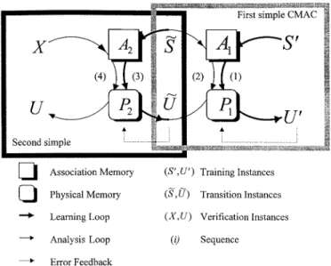
FIG. 2. Time inversion CMAC Neural Network with Two Con-nected Simple CMACs
where the superscript (k⫹ 1) is used to indicate the (k ⫹ 1)th learning step; and the quantity = predefined learning ratio. In this work, is set as a real number in the interval of [0, 1] instead of 1.0 in Albus’s work. The learning phase is ter-minated as the predefined stopping criterion is met.
Time Inversion CMAC Neural Network
A simple CMAC neural network has the property of fast convergence in learning phase (Albus 1975a). However, the prediction performance of a well-trained CMAC neural net-work in verification phases is extremely dependent upon some predefined working parameters, such as the size of association memory A and physical memory P used. To improve the per-formance of CMAC neural network learning models, Albus (1975b) proposed a time inversion technique to refine com-putations in a simple CMAC.
For instance, a set of instances, S⬘(x⬘, y⬘, z⬘, u⬘, v⬘, w⬘), with six decision variables in input and the corresponding output
U⬘ are given. An unsolved instance, X(x, y, z, u, v, w), is used
as a verification instance. Then, the problem can be solved by a time inversion CMAC with two connected simple CMACs as shown in Fig. 2. The computations of the time inversion CMAC neural network can be summarized as the following steps:
• Step 1. S⬘(x⬘, y⬘, z⬘, u⬘, v⬘, w⬘) and U⬘ are used to train the first simple CMAC of the time inversion CMAC ac-cording to the aforementioned three sequential mappings,
S →A, A→P, and P →U.
• Step 2. The outputU˜ corresponding toS(x˜ ⬘,y⬘, z⬘, u, v, w) is computed using the first trained simple CMAC using
(1). Herein, the instances[S(x˜ ⬘,y⬘, z⬘, u, v,w)U ]˜ are called transition instance.
• Step 3. S(x˜ ⬘,y⬘, z⬘, u, v, w) and U˜ are used as training instances to train the second simple CMAC of the time inversion CMAC.
• Step 4. Finally, the output U corresponding to X(x, y, z,
u, v, w) is computed through the second simple CMAC.
The aforementioned four steps are denoted as Sequences (1) and (2) in the first CMAC and Sequences (3) and (4) in the second CMAC in Fig. 2, respectively.
MS㛭CMAC NEURAL NETWORK LEARNING MODEL
This work presents a novel MS㛭CMAC neural network learning model. The learning algorithm associated with the
proposed model is based on the concept of dimensional re-duction. Hence, connecting a number of time inversion CMACs as a tree structure allows us to construct the topology of the MS㛭CMAC. Hereinafter, the learning algorithm of an MS㛭CMAC neural network is explicated with a simple ex-ample with three decision variables x, y, and z. The following combinations of three decision variables are considered as training instances:
x = {x , x , x }1 2 3
y = {y , y , y }1 2 3
z = {z , z , z }1 2 3 Thus, this example contains a total of 27 (33
) distinct training instances. A vector X(xu, yu, zu) is the input of any verification instance.
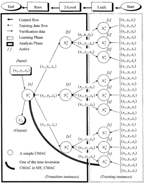
The problem can be solved using an MS㛭CMAC neural network with a three-level tree structure schematically de-picted in Fig. 3. Each node of the tree denotes a simple CMAC neural network. The link between any two connected nodes indicates the data flow. Cumulatively, the tree contains 12 links.
After the topology of the MS㛭CMAC neural network is de-rived, the training instances are divided into nine groups and presented to the leaves. Simultaneously, the verification in-stance is presented to the root. Each node in the level two and the leaves is only fed a transition instance during the verifi-cation phase. Restated, this case contains 12 transition in-stances. After the output of each transition instance is com-puted through a corresponding node, the transition instances are used in the training phase of the node’s parent. In each node, only one input pattern is considered as a key-mapping variable. The input pattern is referred to herein as an active parameter. Notably, the active parameter differs according to each level. Herein, these parameters are x, y, and z in root, level two, and leaf, respectively.
The computations, then, of the MS㛭CMAC neural network can be implemented in three stages. First, consider the decision variable z as the active parameter. Nine transition instances can be generated. Each transition instance is computed by means of a simple CMAC trained by three of the training instances. Hence, the original three-dimensional (3D) problem is reduced to a two-dimensional (2D) problem.
Next, another variable (i.e., y) is considered as the active parameter in this stage. Three new transition instances can be generated by means of the aforementioned nine transition stances using three simple CMACs. Each new transition in-stance is computed by a simple CMAC trained by three tran-sition instances generated in the first stage. Therefore, in this work, the 2D problem is altered to a one-dimensional (1D) problem only.
In the final stage, the output of the verification instance x can be computed by a simple CMAC (i.e., trained using the three transition instances generated in the second stage). In-stead of using 27 training instances to map a verification in-stance in a 3D domain, the verification inin-stance is mapped using three transition instances in a 1D space.
Computational performance in an MS㛭CMAC neural net-work depends on the number of given training instances. As-sume that the decision variables x, y, and z have N distinguish-able values; there are N3
distinguishable possible training instances. To resolve this problem, an amount of N3 associa-tion memory A spaces is required by using a simple CMAC neural network at least. However, only 13N (N ⫹ 3N ⫹ 9N) association memory A spaces are used in an MS㛭CMAC neu-ral network. Obviously, the amount of association memory spaces used for solving the problem is significantly reduced in the MS㛭CMAC neural network. Consequently, the
FIG. 3. Topology of Three-Level MS㛭CMAC Neural Network sponding computational time can be substantially reduced in
a certain order.
More detailed notations about the MS㛭CMAC neural net-work are characterized in the following. In general, the number of levels in an MS㛭CMAC tree structure is set equal to the number of decision variables in an input. Each training in-stance is represented as S⬘(s⬘ , s⬘ ,1, t1 2, t2 . . . , s⬘ )n, tn in an input, where si, t⬘i = {s⬘ 兩ti, ti i = 1 to pi}, 1 ⱕ i ⱕ n. The term pi is a predefined constant. Then, the topology of the tree of MS㛭 CMAC can be defined as follows:
• The hth node in ith level of tree is denoted as i
N .h • The number of nodes in ith level can be set as
1 if i = 1 i⫺1
p¯ =i
再
(3)pj if i > 1
写
j =1• There are pi children (nodes) for node where 1 ⱕ i i
N ,h
ⱕ n ⫺ 1 and 1 ⱕ h ⱕ p¯l.
• Cumulatively, the tree contains p¯nleaves (nodes) that are denoted as where 1ⱕ c ⱕ p¯n.
n
N ,c
If a new instance X(s , s ,1, u 2, u . . . , s )n, u is given, then the corresponding output Uu can be obtained using the MS㛭 CMAC neural network learning model according to the fol-lowing steps:
• Step 1: Use instance X as a verification instance in 1
N1 node. The training instances ofNn are selected from the
c
given training instance set. Subscript ti (i = 1 to n⫺ 1) ofS⬘(s⬘ , s⬘ ,1, t1 2, t2 . . . , s⬘ )n, tn is computed as follows:
t = {1, 2, . . . , p }n n
c = cn for i = 1 to n ⫺ 1
pn⫺i if cn⫺i⫹1mod pn⫺i= 0
tn⫺i=
再
c mod p else (4a)n⫺i⫹1 n⫺i
Cn⫺i= (Cn⫺i⫹1⫺ t )/pn⫺i n⫺i⫹ 1 (4b) • Step 2: Generate transition instances in the tree. The input
in the transition instance of l is defined as follows:
Nb ˜S = S*T ⫹ XUl l (5a) Il⫺1 0 T =l
冋 册
(5b) 0 0 n⫻n 0 0 U =l冋 册
(5c) 0 In⫺l⫹1 n⫻nwhere Ij= j⫻ j identify matrix; S* = any training instance of nodeN ;l X = verification instance of MS㛭CMAC
neu-b
ral network; and ˜S= verification instance of node l
N .b • Step 3: Perform the learning and verification phases of
all simple CMACs from leaves to root. Herein, a binary
JOURNAL OF COMPUTING IN CIVIL ENGINEERING / JANUARY 1999 / 5
TABLE 1. Binary Valuable Table with g = 4 Si (1) ␣1 (2) ␣2 (3) ␣3 (4) ␣4 (5) ␣5 (6) ␣6 (7) ␣7 (8) ␣8 (9) ␣9 (10) ␣10 (11) ␣11 (12) ␣12 (13) 1 1 1 1 1 0 0 0 0 0 0 0 0 2 0 1 1 1 1 0 0 0 0 0 0 0 3 0 0 1 1 1 1 0 0 0 0 0 0 4 0 0 0 1 1 1 1 0 0 0 0 0 5 0 0 0 0 1 1 1 1 0 0 0 0 6 0 0 0 0 0 1 1 1 1 0 0 0 7 0 0 0 0 0 0 1 1 1 1 0 0 8 0 0 0 0 0 0 0 1 1 1 1 0 9 0 0 0 0 0 0 0 0 1 1 1 1
FIG. 4. Learning Results for 1D Example with Different␥ Val-ues
variable table proposed by Albus (1975a) is used in the mapping S→A of any simple CMAC in the MS㛭CMAC
neural network learning model. For instances, Table 1 lists a binary variable table with g = 4. Hence, the function
S㛭A(S*) used in node l is shown as follows:
Nb
* * *
␣* = S㛭A(S*) = {␣ 兩␣ = s ⫹ i, i = 1 to g}i i l (6) wheres*l denotes the lth element of S*. The subsequent mapping of A → P for any simple CMAC in the MS㛭
CMAC neural network learning model is set as follows:
* * *
* = A㛭P(␣*) = { 兩 = ␣ , j = 1 to g}j j j (7) Herein, the process of training in leaves is called the learn-ing phase of an MS㛭CMAC neural network. The other pro-cesses are then called the verification phase of an MS㛭CMAC neural network. Notably, although the learning phase can run in off-line, the verification phase should be run in on-line.
In simple and time inversion CMAC neural networks, the size of A is always hundreds or thousands times larger than the size of P. However, the ratio of the size of A over P equals 1 in an MS㛭CMAC neural network learning model. Further-more, the jth row vector of physically memory Pj computed by (1) for a simple or time inversion CMAC neural network is a step function of j and listed as follows:
W1 if 1ⱕ j < x1
W2 if x1ⱕ j < x2
P =j
再
⭈⭈ ⭈⭈⭈ ⭈
Wa if xa⫺1ⱕ j ⱕ r
where Wi represents a scale vector, i = 1 to a. The basis of computation in (1) is then a linear approach. To strengthen the precision in computational ability in an MS㛭CMAC neural network, a novel quadratic approach is proposed herein. The
jth row vector of physically memory Pjis then augmented as:
j 1 W1⫹
冉 冊
⫺ (W2⫺ W ) ⫻ ␥1 if 1ⱕ j < x1 x1 2 j⫺ xi⫺1 1 P =j Wi⫹冉
⫺冊
(Wi⫹1⫺ W ) ⫻ ␥ if xi⫺1 i⫺1ⱕ j < xi xi⫺ xi⫺1 2 j⫺ xa⫺1 1 Wa⫹冉
⫺冊
(Wa⫺1⫺ W ) ⫻ ␥a if xa⫺1ⱕ j ⱕ r r⫺ xa⫺1 2 (8) where␥ = real number in the interval of [0, 1]. For instance, a 1D function y(x) with five given points, denoted as solid circles in Fig. 4, is given. Fig. 4 also displays three mapped functions with three different values of ␥ based on the five given points by means of an MS㛭CMAC neural network.COMPARISON OF TIME INVERSION CMAC AND
MS㛭CMAC NEURAL NETWORK
The example of design of concrete beams was first solved by a back-propagation neural network with five parameters Mu,
b/d,, fy, andf⬘c in inputs and one data d in output (Vanluchene and Sun 1990). Where Mu is the ultimate bending moment; b and d are the width and depth of a rectangular section, re-spectively; is the reinforcement ratio; fyis the yielding stress of reinforcement; andf⬘c is the compress strength of concrete. The relation between input and output can be expressed as follows:
fy 2
M = bd fu ⬘(1 ⫺ 0.59); =c (9a,b) f⬘c
Gunaratnam and Gero (1994) solved the example by using the technique of dimensionless analysis to improve the per-formance of a back-propagation neural network. Adeli and Park (1995) used the same dimensionless data set as training instances of a CPN. For the sake of comparison of the learning performances of a time inversion CMAC and an MS㛭CMAC neural network learning models, a large example of 7,540 training instances, with the aforementioned five patterns in in-puts and one data in outin-puts, was created. The instances were divided into two sets: 2,940 training instances and 4,620 ver-ification instances. The verver-ification instances are, then, equally divided into two groups, Test 1 and Test 2.
The input data corresponding to the five parameters of train-ing instances are set as follows: Mu is changed from 226 to 474.6 kN⭈m with increments of 22.6 kN⭈m; b/d is changed from 0.5 to 0.8 with increments of 0.05; is changed from 0.012 to 0.028 with increments of 0.004; fy is changed from 2,800 to 4,200 kg/cm2 with increments of 700 kg/cm2 ; and is changed from 210 to 350 kg/cm2 with increments of 70 f⬘c
kg/cm2. For verification instances in Test 1, M
u is changed from 237.3 to 463.3 kN⭈m with increments of 22.6 kN⭈m, and the other four variables in input are the same as training instances. For verification instances in Test 2, Mu is changed from 237.3 to 463.3 kN⭈m with increments of 22.6 kN⭈m;
b/d is changed from 0.525 to 0.775 with increments of 0.05;
and the other variables in input are the same as training in-stances. Note that the inputs of instances are linearly trans-formed from real numbers into integer numbers of interval [1, 90], as the approach of the binary value table was employed. Consequently, the combinations of the five parameters in in-puts for training and verification instances are set as follows:
s :Mu {1, 9, 17, 25, 33, 41, 49, 57, 65, 73, 81, 89} (training) {5, 13, 21, 29, 37, 45, 53, 61, 69, 76, 84} (Test 1 and Test 2)
s :b/d {1, 14, 27, 40, 53, 66, 79} (training and Test 1) {7, 20, 33, 46, 59, 72} (Test 2)
FIG. 5. MS㛭CMAC Neural Network for Moment Gradient Coefficient Example
s: {1, 21, 41, 61, 81} (training, Test 1, and Test 2)
s :fy {1, 41, 81} (training, Test 1, and Test 2)
s :fc⬘ {1, 41, 81} (training, Test 1, and Test 2)
First, the example is solved by a time inversion CMAC neural network with two connected simple CMACs. Working parameters were set as follows: The maximum learning itera-tion is set as 50, generalizaitera-tion size g is set as 50, and the size of physical memory P is set as 14,700. The instances in Test 1 were used as the transition instances in first connected simple CMAC. The instances in Test 2 were, then, used as verification instances in the second connected simple CMAC. It took about 274 s of computing time on a DEC 3000 workstation. The average percentage errors in prediction of the verification in-stances are 2.19 to Test 1 and 3.13 to Test 2.
Then, the example was solved using a five-level MS㛭 CMAC neural network learning model. The active parameters for Levels 5 to 1 were set as Mu, b/d,, fy, andf⬘,c respectively. The generalization size g was set as 50, 50, 50, 40, and 40 in Levels 5 to 1, respectively. The term␥ is set as 0.5 in all five levels. The outputs of instances in Test 1 were calculated from nodes in Level 5, and the outputs of instances in Test 2 were calculated from nodes in Level 2. Accordingly, the average percentage errors in prediction verification instances are 0.64 for Test 1 and 1.28 for Test 2. It took only 24 s of computing time on a DEC 3000 workstation. In sum, the comparing re-sults indicate not only a superprediction performance in veri-fication instances but also a substantial decrease in computing time for the MS㛭CMAC neural network learning model as compared with a time inversion CMAC neural network.
APPLICATIONS
Two steel structural design examples were used to assess the performance of the MS㛭CMAC neural network learning model. The two examples are the estimation of moment gra-dient coefficient in steel beams and the determination of ef-fective length of columns in unbraced frames, respectively. The computations for these two examples are complicated in structural engineering. Moreover, the two examples are gen-erally solved by conventional numerical computing ap-proaches.
Moment Gradient Coefficient Cbfor Monosymmetric
Steel Beams Subjected to End Moments
In the American Institute of Steel Construction’s Load
Re-sistance Factor Design (LRFD) specifications (Manual 1994),
the maximum buckling moment Mc r in monosymmetric steel beam subjected to a gradient distributed moment can be ap-proximately calculated by the following equations:
2
Mc r= C M ;b u m C = 1.75b ⫹ 1.05 ⫹ 0.3 ⱕ 2.3 (10a,b) where Cb = real number called moment gradient coefficient;
Mu m= buckling moment in monosymmetric steel beam sub-jected to a uniformed moment; and = M1/M2 = ratio of two end moments, in which M1 is the smaller end moment.
A more conservative method to calculate Cbis suggested by Kitipornchai (1985), and it is expressed as
2 ␥c ¯2 x¯ x¯ C =b
冋
冑
1⫹ 4(1 ⫺ )k ⫹冉 冊
k ⫹ k册
(11) h h where x/h = 0.9(2 ⫺ 1)[1 ⫺ (Iy/Ix) 2 ]; ¯k = = beam parameter; = coefficientmonosym-2 2 2
EI h /4GJLy
兹
metric from inverted T-shape ( = 0) to T-shape ( = 1.0) shown in Fig. 5; and ␥c = monodimensional elastic critical buckling moment. The␥ccan be determined by the Rayleigh-Ritz method using the nine-term Fourier sine series to express deflection and rotation shape (Kitipornchai 1985). It is a find-ing that the lowest positive root problem of a power series of order 18 in term of␥cwith,¯k, and is a coefficient. In this work, the term ␥c was solved by the Rayleigh-Ritz method using MALAB 4.0 on a personal computer.
A three-level MS㛭CMAC neural network is used to predict the moment gradient coefficient Cb. The parameters in input are , ¯k, and . The value of Iy/Ix is set as 0.075 in all in-stances. The following combinations of the three input param-eters are considered as training instances:
: {⫺1.0, ⫺0.8, ⫺0.6, ⫺0.4, ⫺0.2, 0, 0.2, 0.4, 0.6, 0.8, 1.0}
:
¯k {0.5, 1.0, 1.5, 2.0}
: {0, 0.07, 0.2, 0.4, 0.6, 0.8, 0.93, 1.0}
These combinations are then transformed to integer numbers as follows:
s: {1, 11, 21, 31, 41, 51, 61, 71, 81, 91, 101}
¯
s :k {1, 21, 41, 61}
s: {1, 8, 21, 41, 61, 81, 94, 101}
The following combinations of the three input parameters are considered as verification instances:
: {⫺1.0, ⫺0.8, ⫺0.6, ⫺0.4, ⫺0.2, 0, 0.2, 0.4, 0.6, 0.8, 1.0}
JOURNAL OF COMPUTING IN CIVIL ENGINEERING / JANUARY 1999 / 7
¯k: {0.75, 1.25, 1.75}
: {0.1, 0.3, 0.5, 0.7, 0.9}
These combinations are then transformed as integer numbers as follows:
s: {1, 11, 21, 31, 41, 51, 61, 71, 81, 91, 101}
¯
s :k {11, 31, 51}
s: {11, 31, 51, 71, 91}
Thus, there are a total of 517 instances created and divided into two sets: 352 training instances and 165 verification in-stances. The active parameters for Levels 3 to 1 in the three-level MS㛭CMAC neural network were , ¯k, and , respec-tively. Working parameters were set as follows: ␥ was set as 1.0, 0.5, and 0 in Levels 3 to 1, respectively, and the gener-alization size g was set as 100, 60, and 20, respectively.
The computing results are shown in Figs. 6(a – c), respec-tively. The average percentage error for 165 verification in-stances is 0.56. The two largest percentage errors in verifica-tion instances are 4.94 (as¯k= 0.75, = 0.9, and  = 1.0) and 4.92 (as ¯k= 1.75, = 0.1, and  = 0.4). Notably, the results are within the acceptable limits in an engineering design com-putation. Note that the MS㛭CMAC neural network learning model has excellent prediction performance, with the average error of 0.22%, as 0.1 < < 0.9. Notwithstanding, the com-puting results for high monosymmetric I-beams ( ⱖ 0.9 or
ⱕ 0.1) with  > 0 and k¯ = 0.75 or k¯ = 1.75, are poor as comparing with other verification instances. However, the is-sue can be improved as the number of training instances in-creased.
Effective Length Factor K of Columns in Unbraced Frames
The inelastic buckling strength of an element subjected to axial loading can be calculated by the following equation:
2 Et
Fc r= 2 (12)
(KL/r)
where Et = tangent modulus of elasticity at critical strength; r is the radius of gyration; and KL is the effective length of columns. In LRFD specifications (Manual 1994), the value of
K can be evaluated by an alignment chart. Recently, Duan and
Chen (1989), as well as Kishi et al. (1997) found that the effective length of columns determined using the alignment chart would be too conservative or not safe with different boundary conditions.
Herein, a subassemblage model of an unbraced frame based on the alignment chart approach is established. The model is composed of Column c2 with two ends A and B, two restrained columns (c1 and c3), and four restrained beams. Column c1 and two of the beams are rigidly connected to the end A. Meanwhile, Column c3 and the two other beams are rigidly connected to the end B. Herein, the far ends of c1 and c3 are rigidly or fixed connected. The general governing equations for the K factor of Column c2 can be derived as (Kishi et al. 1997)
a11 a12 a13
det a
冏
21 a22 a23冏
= 0 (13a) a31 a32 a33and the entries ai j, i = 1 to 3 and j = 1 to 3 are defined as 2 6 si j a11= si i⫹ ⫺ GAc1 ; a12= GAc 2 i js (13b,c) G⬘A si i si j a13=⫺(s ⫹ s ) 1 ⫺ Gi i i j
冉
Ac1冊
(13d ) si i 2 6 si j a21= GBc 2 i js ; a22= si i⫹ ⫺ GBc 3 (13e, f ) G⬘B si i si j a23=⫺(s ⫹ s ) 1 ⫺ Gi i i j冉
Bc 3冊
(13g) si i 2 a31= a32= si i ⫹ s ; a = (/K) ⫺ 2(s ⫹ s )i j 33 i i i j (13h,i ) where (EI/L)c (EI/L)c冘
A冘
B G⬘ =A ; G⬘ =B (14a,b) ␣ (EI/L)u f b ␣ (EI/L)u f b冘
A冘
B (EI/L)c i (EI/L)c iGAci= ; GBci= (15a,b)
(EI/L)c (EI/L)c
冘
A冘
B 2 sin ⫺冉 冊
cos K K K K s =i i (16a) 2⫺ 2 cos ⫺ sin K K K 2 ⫺ sin冉 冊
K K K s =i j (16b) 2⫺ 2 cos ⫺ sin K K KIn the previous equations, subscripts A and B in G⬘ indicate the columns and beams connected at the Ath and Bth nodal points, respectively. Subscripts b and c denote beam and umn, respectively. Subscript ci (i = 1 or 2 or 3) indicates col-umn number.
In this example, two boundary conditions are examined. They are both far ends of c1 and c3 fixed (K1) and rigid con-nected (K2). Table 2 lists the values of GAciand GBci. There are two input parameters(G⬘, G⬘)A B and two output data (K1, K2) in each instance. The following combinations of two input pa-rameters are considered as training instances:
{1, 2, 3, 4, 5, 6, 7, 8, 9, 10}
G⬘, G⬘:A B
The parameters are then linearly transferred to integers in the interval of [1, 91] as follows:
{1, 11, 21, 31, 41, 51, 61, 71, 81, 91}
s ,G⬘A s :G⬘B
The following combinations of two input parameters are con-sidered as verification instances:
{1.5, 2.5, 3.5, 4.5, 5.5, 6.5, 7.5, 8.5, 9.5}
G⬘, G⬘:A B
The corresponding combinations of the two parameters in transformed integer numbers are then set as follows:
{6, 16, 26, 36, 46, 56, 66, 76, 86}
s ,G⬘A s :G⬘B
Thus there are a total of 181 instances created using MALAB 4.0 on a personal computer and divided as 100 training in-stances and 81 verification inin-stances. Note that the K-factor is set as 10 when the value of computed K exceeds 10 in this work. A two-level MS㛭CMAC neural network was used to solve this example. The active parameters areG⬘A in leaf and in root. The generalization size g was set as 50 in leaf and
G⬘B
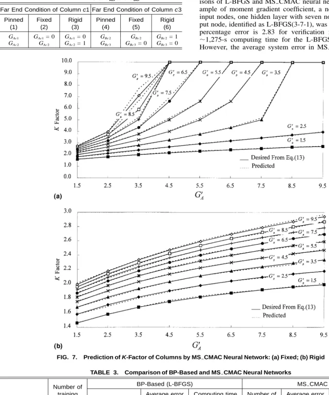
root, respectively, and the term ␥ was set as 0.6 in Levels 2 and 1. The learning results are shown in Figs. 7(a and b).
The average percentage errors in K1 and K2 are 0.67 and
FIG. 6. Prediction of Moment Gradient Coefficient by MS㛭CMAC Neural Network for: (a)k¯= 0.75; (b)k¯= 1.25; (c)k¯= 1.75
JOURNAL OF COMPUTING IN CIVIL ENGINEERING / JANUARY 1999 / 9
TABLE 3. Comparison of BP-Based and MS㛭CMAC Neural Networks
Examples (1) Number of training instances (2) BP-Based (L-BFGS) Topology (3) Average error (%) (4) Computing time (s) (5) MS㛭CMAC Number of branch (6) Average error (%) (7) Computing time (s) (8) Cb[Eq. (11)] 352 L-BFGS(3-7-1) 2.83 1,275 R a-11-5 0.56 21 K-factor (rigid) 100 L-BFGS(2-5-1) 0.52 48 Ra -10 0.37 3 K-factor (fixed) 100 L-BFGS(2-5-3-1) 0.89 102 — 0.67 — Note: BP = back-propagation. aR = root.
FIG. 7. Prediction of K-Factor of Columns by MS㛭CMAC Neural Network: (a) Fixed; (b) Rigid TABLE 2. Values of GAciand GBci
Far End Condition of Column c1 Pinned (1) Fixed (2) Rigid (3)
Far End Condition of Column c3 Pinned (4) Fixed (5) Rigid (6) GAc1 GAc1= 0 GAc1= 0 GBc 2 GBc 2 GBc 2= 1 GAc 2 GAc 2 GAc 2= 1 GBc 3 GBc 3= 0 GBc 3= 0 0.37, respectively. Kishi et al. (1997) reported that the errors of K-factor determined using the LRFD specification (Manual 1994) alignment chart were ⫺2.6 to ⫺56.6% for fixed-fixed boundary,⫺1.2 to ⫺17.6% for fixed-rigid boundary, and 8.2 to 14.4% for pinned-pinned boundary. Herein, the learning re-sults confirm that the MS㛭CMAC neural network learning model has excellent prediction performance for K-factors of
columns in unbraced frames. In addition, the prediction results are within the acceptable limits in an engineering design com-putation.
Comparison of L-BFGS and MS㛭CMAC Neural
Networks
Herein, the two examples were then solved using L-BFGS supervised neural networks. Table 3 summarizes the compar-isons of L-BFGS and MS㛭CMAC neural networks. In the ex-ample of moment gradient coefficient, a network with three input nodes, one hidden layer with seven nodes, and one out-put node, identified as L-BFGS(3-7-1), was used. The average percentage error is 2.83 for verification instances. It took
⬃1,275-s computing time for the L-BFGS neural network.
However, the average system error in MS㛭CMAC is 0.56%
for verification instances. It took only 21-s computing time for the MS㛭CMAC neural network. Notably, the problem is taken from the literature (Adeli and Park 1995). The training and verification instances, however, are entirely distinct to their work. Hence, no computational comparison is made between the MS㛭CMAC and CPN neural networks.
In the example of estimate K-factor, a network with two input nodes, one hidden layer with five nodes, and one output node (2-5-1) was used in the cases of rigid-rigid boundary. In addition, a network with two input nodes, two hidden layers with five and three nodes, and one output node (2-5-3-1) was used in the cases of fixed-fixed boundary. The average percentage errors for verification instances with two different boundaries are 0.52 and 0.89, respectively. It took about 48 and 102 s, respectively, for L-BFGS neural networks in two boundary conditions. However, the average percentage errors were 0.37 and 0.67 for verification instances, respectively, and the computing time in MS㛭CMAC neural network is only 3 s.
CONCLUSIONS
This work presents a novel supervised neural network learn-ing mode, MS㛭CMAC learning model, by connecting a large number of time inversion CMAC as a topology of tree struc-ture. The MS㛭CMAC neural network learning model proposed herein applied to engineering design problems. Two structural engineering problems are addressed to assess the learning per-formance of the MS㛭CMAC neural network learning model. Based on the results in this work, we can conclude the follow-ing:
1. The MS㛭CMAC neural network learning model can be used to solve structural engineering problems that are generally solved by numerical computing approaches within a reasonable central processing unit time. These numerical approaches, however, are not readily available for structural engineers to use. Moreover, the computing results in the MS㛭CMAC neural network learning model are more precise than that estimated through approximate charts in LRFD specifications.
2. The prediction performance of the MS㛭CMAC neural network learning model is superior to that of L-BFGS supervised neural networks for verification instances. Moreover, more additional learning cycles are often re-quired to train the neural network when a new instance is added into the training sets for L-BFGS supervised learning models. However, the issue of additional learn-ing cycles for trainlearn-ing is circumvented in the MS㛭CMAC neural network learning model. Only the associated physical memory corresponding to the new training in-stance needs to be updated.
3. For a time inversion CMAC neural network, the sizes of
A and P must be large enough for performing good
prediction in verification phase. The size of A is always hundreds or thousands times larger than the size of P. However, in the MS㛭CMAC neural network learning model, the size of A is significantly reduced and the ratio of the size of A over P is equal to 1. As a result, the MS㛭CMAC neural network learning model can converge quickly to an accepted solution in a few iterations.
4. A time inversion CMAC neural network uses a linear interpolation approximation to calculate the adjustments for updating the physical memory. Hence, for a nonlinear problem, the performance of verification is poor in a time inversion CMAC neural network. A novel approach for calculating the adjustment in updating physical memory
is presented in this work. Instead of the linear interpo-lation approximation, a quadratic interpointerpo-lation approxi-mation (trapezium schema) is utilized in the MS㛭CMAC neural network learning model. Significant improvement in the learning performance for verification instances is achieved in the MS㛭CMAC neural network learning model.
ACKNOWLEDGMENTS
The writers would like to thank the National Science Council of the Republic of China for financially supporting this research under Contract No. NSC 87-2211-E-009-029.
APPENDIX. REFERENCES
Adeli, H., and Hung, S. L. (1993). ‘‘A concurrent adaptive conjugate gradient learning algorithm on MIMD shared memory machines.’’ J.
Supercomp. Appl., 7(2), 155 – 166.
Adeli, H., and Hung, S. L. (1994). ‘‘An adaptive conjugate gradient learn-ing algorithm for effective trainlearn-ing of multilayer neural networks.’’
Appl. Mathematics and Computation, 62(1), 81 – 102.
Adeli, H., and Park, H. S. (1995). ‘‘Counterpropagation neural networks in structural engineering.’’ J. Struct. Engrg., ASCE, 121(8), 1205 – 1212.
Albus, J. S. (1975a). ‘‘A new approach to manipulator control: The cer-ebellar model articulation controller (CMAC).’’ J. Dyn. Sys.,
Measure-ment, and Control, 97(3), 220 – 227.
Albus, J. S. (1975b). ‘‘Data storage in the cerebellar model articulation controller.’’ J. Dyn. Sys., Measurement, and Control, 97(3), 228 – 233.
Duan, L., and Chen, W. F. (1989). ‘‘Effective length factor for columns in unbraced frames.’’ J. Struct. Engrg., ASCE, 115(1), 149 – 165. Elkordy, M. F., Chang, K. C., and Lee, G. C. (1994). ‘‘A structural
dam-age neural network monitoring system.’’ Microcomp. in Civ. Engrg., 9(2), 83 – 96.
Ghaboussi, J., Garrett, J. H., and Wu, X. (1991). ‘‘Knowledge-based mod-eling of material behavior and neural networks.’’ J. Engrg. Mech., ASCE, 117(10), 132 – 153.
Goh, A. T. C. (1995). ‘‘Back-propagation neural networks for modeling complex systems.’’ Artificial Intelligence in Engrg., 9(1), 143 – 151. Gunaratnam, D. J., and Gero, J. S. (1994). ‘‘Effect of representation on
the performance of neural networks in structural engineering applica-tions.’’ Microcomp. in Civ. Engrg., 9(2), 97 – 108.
Hajela, P., and Berke, L. (1991). ‘‘Neurobiological computational modes in structural analysis and design.’’ Comp. and Struct., 41(4), 657 – 667. Hecht-Nielsen, R. (1987). ‘‘Counterpropagation networks.’’ Appl. Optics,
26(3), 4979 – 4984.
Hung, S. L., and Adeli, H. (1993). ‘‘Parallel back propagation learning algorithm on Cray YMP8/864 supercomputers.’’ Neurocomputing, 5(6), 287 – 302.
Hung, S. L., and Adeli, H. (1994). ‘‘A parallel genetic neural network learning algorithm for MIMD shared memory machines.’’ IEEE Trans.
On Neural Networks, 5(6), 900 – 909.
Hung, S. L., and Jan, J. C. (1997). ‘‘Machine learning in engineering design — an unsupervised fuzzy neural network case-based learning model.’’ Proc., Intelligent Information Sys., IEEE Computer Society, Los Alamitos, Calif., 156 – 160.
Hung, S. L., and Lin, Y. L. (1994). ‘‘Application of an L-BFGS neural network learning algorithm in engineering analysis and design.’’ Proc.,
2nd Nat. Conf. on Struct. Engrg., Chinese Soc. of Struct. Engrg.,
Nan-tou, Taiwan, R.O.C., 221 – 230.
Kasperkiewicz, J., Racz, H., and Dubrawski, A. (1995). ‘‘HPC strength prediction using artificial neural network.’’ J. Computing in Civ.
Engrg., ASCE, 9(4), 279 – 284.
Kishi, N., Chen, W. F., and Goto, Y. (1997). ‘‘Effective length factor of columns in semirigid and unbraced frames.’’ J. Struct. Engrg., ASCE, 123(3), 313 – 320.
Kitipornchai, S., Wang, C. M., and Trahair, N. S. (1986). ‘‘Buckling of monosymmetric I-beams under moment gradient.’’ J. Struct. Engrg., ASCE, 112(4), 781 – 799.
Lin, C.-S., and Chiang, C. T. (1997). ‘‘Learning convergence of CMAC technique.’’ IEEE Trans. Neural Networks, 8(6), 1281 – 1292.
JOURNAL OF COMPUTING IN CIVIL ENGINEERING / JANUARY 1999 / 11 Manual of steel construction — load and resistance factor design. (1994).
American Institute of Steel Construction, Chicago.
Mukherjee, A., and Deshpande, J. M. (1995). ‘‘Modeling initial design process using neural network.’’ J. Computing in Civ. Engrg., ASCE, 9(3), 194 – 200.
Nocedal, J. (1990). ‘‘The performance of several algorithms for largescale unconstrained optimization.’’ Large-scale numerical optimizaion,
T. F. Coleman, and Y. Li, eds., Soc. for Industrial and Applied Math., Philadelphia, 138 – 151.
Rumelhart, D., Hinton, G., and Williams, R. (1986). ‘‘Learning represen-tations by back-propagation errors.’’ Parallel distributed processing, D. Rumelhart et al., eds., Vol. 1, MIT Press, Cambridge, Mass., 318 – 362. Vanluchene, R. D., and Sun, R. (1990). ‘‘Neural networks in structural
engineering.’’ Microcomp. in Civ. Engrg., 5(3), 207 – 215.