國 立 交 通 大 學
電 控 工 程 研 究 所
碩 士 論 文
利 用 嵌 入 式 繼 光 鏡 顯 微 超 頻 譜
影 像 系 統 進 行
口
腔
癌 檢
測
Detection of oral cancer using embedded relay lens
microscopic hyperspectral imaging system (ERL-MHIS)
研 究 生:陳 誌 賢
指導教授:歐 陽 盟 教授
.
利用嵌入式繼光鏡顯微超頻譜影像系統進行口腔癌檢測
Detection of oral cancer using embedded relay lens microscopic hyperspectral
imaging system (ERL-MHIS)
研 究 生:陳誌賢 Student:Chih-Hsien Chen 指導教授:歐陽盟 Advisor:Mang Ou-Yang 國 立 交 通 大 學 電控工程研究所 碩 士 論 文 A Thesis
Submitted to Institute of Electrical Control Engineering College of Electrical and Computer Engineering
National Chiao Tung University in partial Fulfillment of the Requirements
for the Degree of Master
in
Electrical Control Engineering
October 2012
Hsinchu, Taiwan, Republic of China
利用嵌入式繼光鏡顯微超頻譜影像系統進
行口腔癌檢測
學生 : 陳誌賢 指導教授 : 歐陽盟 教授 國立交通大學電控工程研究所摘要
癌症在國人十大死因的榜首居高不下,其中口腔癌是惡性腫瘤中最可能 早期發現,並且藉由早期治療進而痊癒。相較於傳統檢測方法,以肉眼判 斷是否有癌症細胞的侵蝕,高光譜影像提供了更多的資訊。我們以嵌入式 繼光鏡高光譜成像系統(ERL-MHIS)對細胞切片樣本進行掃描,建立一個三 維高光譜資訊矩陣,並且提出了型態與光譜兩類方法進行癌症的辨識。在 癌症細胞的影像型態判斷方面,我們提出兩種方法,第一個方法為使用臨 界值分離出細胞的基底層,並且使用碎形維度(fractal dimension)計算維度, 因為癌症細胞的分裂失去限制,分維的維度值會較正常細胞的維度高。當 口腔黏膜細胞發生癌病變時,基底層細胞會持續向內部的固有層持續侵 蝕,造成固有層的型態產生變化,因此第二種方法為使用 K 最鄰近分類算 法(KNN)對固有層的細胞核影像做分類,並且計算分類結果的準確率。光譜 判斷方面,使用了光譜強度的比值、半波寬度(FWHM)、波形下面積與光譜 波段範圍內的強度。將分析結果使用高斯分佈計算準確率。我們將準確率 高的前三個方法做結合,並且計算新的準確率 98.45%.最後,藉由考慮樣本 資料,我們提出雞尾酒方法,將判斷癌症之螢光光譜的準確率提升到 87%。Early detection of oral cancer using embedded relay
lens microscopic hyperspectral imaging system
(ERL-MHIS)
student:Chih-Hsien Chen Advisor:Mang O u-Yang
Institute of Electrical Control Engineering National Chiao Tung University
Abstract
Cancer has been the leading cause of death for years in Taiwan. Oral cancer has the greatest possibility for early detection and recovery after early treatment. Compared to the traditional method of using the naked eye to detect oral cancer, the method of using the hyperspectral image of tissue can offer more information. We used the embedded relay lens microscopic hyperspectral imaging system to scan the sections and save the hyperspectral image. In this study, we diagnosed oral cancer using two methods: morphology and spectrum. In diagnosis using morphology, we presented two techniques: calculation of the fractal dimension and classification of k-Nearest Neighbor (KNN). In diagnosis using the spectrum method, we presented six techniques: comparing intensity, ratio of intensity, wavelength of peak, area under spectral curve, maximum after spline and full width at half maximum. We calculated the sensitivity and specificity using Gaussian distribution. Combining the 3 methods of the highest specificity provides a specificity of 98.45%. Finally, in accordance with sample data, we presented a cocktail method to increase the specificity of spectral analysis with fluorescence excitation to 87%.
Acknowledgement
在研究所兩年之碩士生涯,首先要感謝的人為指導教授 歐陽盟博士不 辭辛勞指導我的研究方向,不時給予鼓勵與支持而讓我持續保有動力來解 決研究過程中所遇到之問題,才能順利完成本論文研究。 感謝 段正仁博士、邱俊誠博士、黃國華博士在繁忙之中抽空給予支 援,願意擔任學生之口試委員,在口試當天提供相當多寶貴意見讓學生可 以清楚瞭解本研究可以改善之處,提升本論文之品質。 接著也要感謝實驗室博班學長庭緯、耀方、昱達與偉德,不論在課業 與研究上面均給予我指導與意見,以及碩士班學長建成,給予研究之建議 以及方法;還有碩士班同學與學弟新淼、智翔、子賢、禹舜、幸璁、冠亨、 益群、浩志、劉穎、俊誠、胤源、碧秀在程式上面給予我許多支援,以及 處理研究相關之大小事,所以讓我在研究所兩年生涯可以過得非常充實以 及順利;感謝我的女友筑羽,持續給我鼓勵與支持,讓我以正向的心態努力 研究。 還有感謝父母在於金錢以及精神上的鼓勵與支持,得以進入研究所學 習更深入之專業技能,讓我可以提升自己,對於在未來踏入競爭如此激烈 之社會,有非常大的幫助以及貢獻。因此在未來進入社會階段,必須持續 保有一顆感恩的心不斷的提升自己、努力向上,使得自己在社會上可以出 人頭地,以報答父母之恩惠。Content
摘要 ... i Abstract ... ii Acknowledgement... iii List of Figures ... vi List of Tables ... ix Chapter 1 Introduction ... 1 1.1 Background information ... 1 1.2 Motivation ... 1Chapter 2 Review Articles ... 3
2.1 Introduction of Anatomy ... 3
2.1.1 Oral cavity ... 3
2.2 Introduction of Histology ... 5
2.2.1 Oral mucosal tissue ... 6
2.2.2 Oral squamous cell carcinoma ... 6
2.2.3 Process of making sections ... 7
2.3 Development of diagnosing cancer using hyperspectral image ... 8
2.3.1 Diagnosis of cancer from image ... 8
2.3.2 Diagnosis of cancer from spectrum ... 9
Chapter 3 Methodology ... 13
3.1 Embedded Relay Lens Microscopic Hyperspectral Imaging System (ERL-MHIS) ... 13
3.2 Process of hyperspectral data ... 14
3.3 Patients and samples ... 15
3.4 Morphological methods for diagnosing oral cancer ... 16
3.4.1 Fractal Dimension ... 17
3.4.2 Classification by K-Nearest Neighbor ... 18
3.5 Spectral methods for diagnosing oral cancer ... 19
3.5.1 Intensity in the specific wavelength range ... 20
3.5.2 Ratio of intensity in two different wavelength ranges ... 23
3.5.3 Wavelength of the specific peak ... 23
3.5.4 Area under spectral curve ... 23
3.5.5 Maximum of spectral curve compensated by spline ... 23
3.5.6 Full Width at Half Maximum (FWHM) of spectral curve ... 24
3.6 Sensitivity and specificity ... 25
Chapter 4 Results ... 27
4.1 Experiments ... 27
4.2.1 Calculation of Fractal Dimension after Threshold Method... 28
4.2.2 K-nearest Neighbor Classification ... 32
4.3 Spectral analysis of oral cancer ... 36
4.3.1 Transmitting spectral mode ... 37
4.3.2 Fluorescence with 330~385nm excitation ... 39
4.3.3 Fluorescence with 470~490nm excitation ... 50
Chapter 5 Discussions, Conclusions and Future Works ... 56
5.1 Discussions ... 56
5.1.1 Cocktail method in accordance to the sample data ... 59
5.1.2 Cause of halogen transmittance over 1.0 ... 67
5.2 Conclusions and future works ... 69
References ... 70
List of Figures
Figure 2-1: The 13 anatomical location. ... 4
Figure 2-2: (a) Well differentiated keratinizing squamous cell
carcinoma. (b) Poorly differentiated keratinizing squamous
cell carcinoma. ... 7
Figure 3-1: The embedded relay lens microscopic hyperspectral
imaging system (ERL-MHIS). ... 14
Figure 3-2: The three dimensional matrix of hyperstral image. ... 15
Figure 3-3: The image (a) of normal tissue and (b) cancer tissue. A:
basal-cell layer B: lamina propria in normal tissue C: cancer
cells D: lamina propria in cancer tissue. ... 16
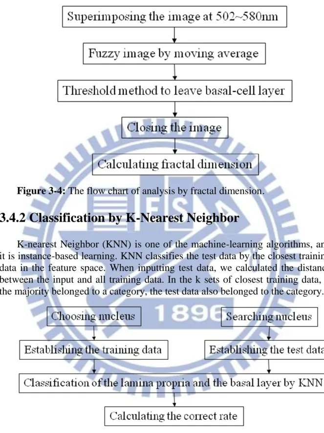
Figure 3-4: The flow chart of analysis by fractal dimension. ... 18
Figure 3-5: The flow chart of analysis by KNN classifying. ... 18
Figure 3-6: Expanding an 11x11 matrix to one dimensional matrix. 19
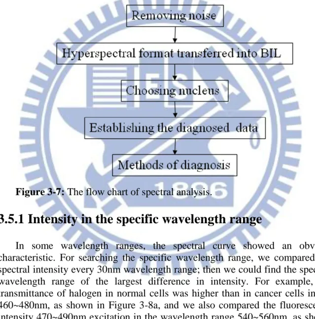
Figure 3-7: The flow chart of spectral analysis. ... 20
Figure 3-8: The spectrum of one sample (a) Halogen transmittance. (b)
Fluorescent intensity with 330-385nm excitation. (c)
Fluorescent intensity compensated by spline with
330-385nm excitation. (d) Fluorescent intensity with
470-490nm excitation. Red line is normal cells, and blue line
is cancer cells. A: the peak in wavelength range 460~480nm.
B: the peak in wavelength range 700~710nm. C: the
intensity in wavelength range 540~570nm. D: the intensity
in wavelength range 680~710nm. E: the maximum of
spectral curve. F: the full width at half maximum (FWHM)
of spectral curve. G: the peak in wavelength range
540~570nm. H: the FWHM of spectral curve. ... 22
Figure 3-9: Spectrum compensated by Spline. Solid line is
fluorescent spectrum with 330-385nm excitation, dotted line
is the spectrum curve compensated by Spline. ... 24
Figure 3-10: Full width at half maximum. ... 25
Figure 3-11: The Gaussian distribution of the analysis. Red line is
normal cells, and blue line is cancer cells. ... 26
Figure 3-12: Calculation of sensitivity and specificity. ... 26
Figure 4-1: The flow chart of experiment ... 28
Figure 4-2: After threshold method, the basal cells are white, and the
others are black in the images. The number 1 to 12 of figure
means the number of the sample. The label (a) means normal
tissue, and the label (b) means cancer tissue. ... 32
Figure 4-3: The result of classification by KNN in the sample
numbered 1 to 12. The number 1 to 12 of figure means the
number of the sample. The label (a) means normal tissue,
and the label (b) means cancer tissue. ... 36
Figure 4-4: The spectral curve of the sample numbered 1 to 12 in
halogen. The red line means normal cells, and blue line
means cancer cells. The number means the number of
patients. X axis is wavelength (nm), and Y axis is halogen
transmittance. ... 39
Figure 4-5: The spectral curves of each sample in fluorescence
330~385nm excitation. The number of figure means the
number of the sample. The red line means normal cells, and
blue line means cancer cells. The number means the number
of patients. X axis is wavelength (nm), and Y axis is
fluorescence intensity (μw). ... 44
Figure 4-6: The spectral curves of each sample which have been
compensated by spline in fluorescence 330~385nm
excitation. The number of figure means the number of the
sample. The red line means normal cells, and blue line
means cancer cells. The number means the number of
patients. X axis is wavelength (nm), and Y axis is
fluorescence intensity (μw). ... 48
Figure 4-7: The spectral curve of each sample in fluorescence
470~490nm excitation. The number of figure means the
number of the sample. The red line means normal cells, and
blue line means cancer cells. The number means the number
of patients. X axis is wavelength (nm), and Y axis is
Figure 5-1: The ratio of people in different age ranges. X axis is
specificity, and Y axis is the ratio of people. ... 60
Figure 5-2: The ratio of people in different differentiation. X axis is
specificity, and Y axis is the ratio of people. ... 61
Figure 5-3: The ratio of people in different locations. X axis is
specificity, and Y axis is the ratio of people. ... 62
Figure 5-4: The ratio of people in different stage. X axis is specificity,
and Y axis is the ratio of people. ... 62
Figure 5-5: The ratio of people in different T. X axis is specificity,
and Y axis is the ratio of people. ... 63
Figure 5-6: The ratio of people in different N. X axis is specificity,
and Y axis is the ratio of people. ... 64
Figure 5-7: The ratio of people in different M. X axis is specificity,
and Y axis is the ratio of people. ... 64
Figure 5-8: The comparison of the methods with vertical bars. ... 67
Figure 5-9: The comparison of spectrum in the halogen and
fluorescence (a) Normal cells in the sample 2. (b) Cancer
cells in the sample 2. (c) Normal cells in the sample 11. (d)
Cancer cells in the sample 11. (e) Normal cells in the sample
12. (f) Cancer cells in the sample 12. The red line means
halogen spectrum, and blue line means fluorescence
spectrum. X axis is wavelength (nm), and Y axis is
List of Tables
Table 2-1: The plane of body ... 3
Table 2-2: The classification of cells ... 5
Table 2-3: Tissue type, disease state, and 516/515nm ratio ... 11
Table 2-4: Fluorescence intensities with 404nm excitation ... 12
Table 2-5: Ratio of fluorescence intensities with 404nm excitation . 12
Table 4-1: The fractal dimension of sample numbered 1 to 12 after
threshold method ... 32
Table 4-2: The correct rate of classification by KNN in the sample
numbered 1 to 12 ... 36
Table 4-3: The number of spectral data ... 36
Table 4-4: The correct rate of classification by KNN in the sample
number 1 to 12 ... 39
Table 4-5: The specificity of analysis in fluorescence 330~385nm
excitation ... 49
Table 4-6: The specificity of analysis in fluorescence 330~385nm
excitation ... 55
Table 5-1: Comparison of other articles ... 58
Table 5-2: The most effective method with each sample data. ... 65
Table 5-3: The combined methods of cocktail method and the
specificity for each sample ... 66
Chapter 1 Introduction
1.1 Background information
The habits of drinking, smoking and betel-nut chewing, in Taiwan have resulted in an increase in the past ten years in the number of people diagnosed with oral cancer. In the last decade, oral cancer was the third leading cause of cancer deaths in Taiwan and number 6 worldwide [1]. Given the high cost and risk in the therapy of terminal oral cancer, early detection is an important issue. The cure rate is 90% in the first stage of oral cancer, 80–90% in the second stage and 30–50% in the third and fourth stages [2]. Traditionally, the method of detecting oral cancer had been to observe the biopsy of the lesions, and then to use a microscope to determine the change in morphology. With the progress of technology, the hyper-spectral scanning system began to be used in observing oral cancer biopsies.
It took twenty years from the invention of the spectrometer for the development of the hyperspectral system. With the spectrometer, the reflected spectrum of different substances was different and provided observers with richer information. The hyperspectral system had the potential to find the relationship between the biochemical and the morphological, and it offered a noninvasive technology to detect oral cancer. Because of its noninvasiveness, it provided rapid detection of oral cancer.
When the change in tissue biochemistry took place, the detected optical characteristic would be influenced. The hyperspectral information in cancer detection included image and spectrum. The analysis of the image was usually done in real time. First, researchers coated the sample with dye, such as hematoxylin. After the light source irradiated the target, the probe could collect information. In some studies, the most helpful feature would be found in the specific excitation wavelength. The autofluorescent spectrum of tissue had been widely used to distinguish cancer from healthy oral mucosa. The methods of spectral analysis included determining: the ratio of intensity in different wavelengths, the intensity in specific wavelength, and the emission and excitation wavelength ratio.
cancer was number 1 in the past 29 years; the average yearly number of deaths caused by cancer was 41,046. In other words, one person died every 13 min as a result of cancer. If the cancer could be detected at an early stage, the cure rate would be increased. The widely used method of detection was observing the biopsies by microscope. Using the naked eye, the medical staffs determined whether the cancer cells had diffused. This method has two shortcomings. First, there would be some error caused by lack of experience in judging cancer tissues. Second, the diagnosis was limited to the spectral bands of visible light: 380~780nm. The data for the hyperspectral image had spectral and spatial information, and the range of wavelength included not only visible light but also near-infrared and ultraviolet. The error caused by inexperience could be avoided if the algorithm comparing the characteristic of the spectrum had been entered into the computer.
In judging cancer tissue, the main basis for observers was whether the basal layer had unlimitedly eroded the lamina propria. The probe diagnosing oral cancer was limited to the surface of the mucosa with low transmittance, so observing the spread of cancer was impossible. If we could combine the analysis of morphology and spectrum, the sensitivity and specificity would be improved.
This research used the hyperspectral scanning system to distinguish cancer cells. We used a microscope to enlarge the image of the sample. There were three light sources: a halogen lamp, a fluorescent lamp with 330~385nm excitation and a fluorescent lamp with 470~490nm excitation. We operated the motor to move the relay lens for scanning the image, and we used the hyperspectrometer to transform the image into a hyperspectral image. The EMCCD would store the hyperspectral image as a three-dimensional matrix. The three axes were x, y and λ. There were four layers in the oral mucosa: the lamina propria, the basal-cell layer, the prickle-cell layer and the keratinized layer. The boundary between the lamina propria and the basal layer became blurred because of the cancer cells’ erosion. We tried to digitalize the image of the cancer and normal tissue. Lastly, we determined the sensitivity and specificity.
Chapter 2 Review Articles
2.1 Introduction of Anatomy
Anatomy is the study of the internal and external structure of the body. Anatomy can be divided into microscopic anatomy and gross anatomy according to the methods of research. Microscopic anatomy uses the microscope to observe the fine structure unobservable with the naked eye. It includes cytology and histology. Gross anatomy means using the naked eye to observe the structure of the body. It includes surface anatomy, regional anatomy and systemic anatomy.
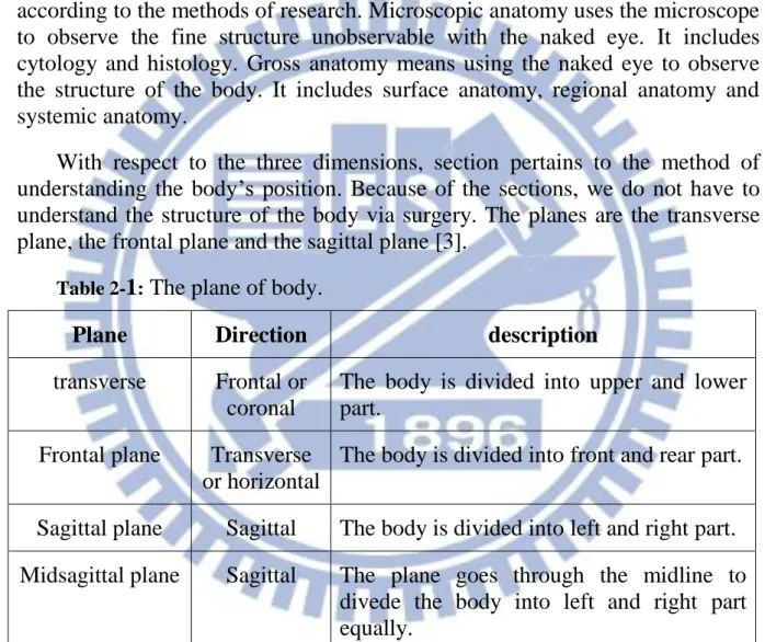
With respect to the three dimensions, section pertains to the method of understanding the body’s position. Because of the sections, we do not have to understand the structure of the body via surgery. The planes are the transverse plane, the frontal plane and the sagittal plane [3].
Table 2-1: The plane of body.
Plane Direction description
transverse Frontal or coronal
The body is divided into upper and lower part.
Frontal plane Transverse or horizontal
The body is divided into front and rear part.
Sagittal plane Sagittal The body is divided into left and right part. Midsagittal plane Sagittal The plane goes through the midline to
divede the body into left and right part equally.
2.1.1 Oral cavity
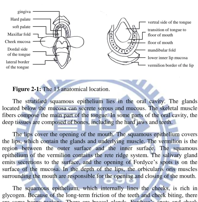
The anatomical locations are the gingival, hard palate, soft palate, maxillar fold, cheek mucosa, dorsal side of the tongue, lateral border of the tongue, ventral side of the tongue, transition of the tongue to the floor of the mouth, the floor of the mouth, the mandibular fold, the lower inner lip mucosa, and the
gingiva Hard palate soft palate Maxillar fold Cheek mucosa Dordal side of the tongue lateral border of the tongue
vertral side of the tongue transition of tongue to floor of mouth floor of mouth mandibular fold lower inner lip mucosa vermilion border of the lip
Figure 2-1: The 13 anatomical location.
The stratified squamous epithelium lies in the oral cavity. The glands located below the mucosa can secrete serous and mucous. The skeletal muscle fibers compose the main part of the tongue. In some parts of the oral cavity, the deep tissues are composed of bones, including the hard jaws and teeth.
The lips cover the opening of the mouth. The squamous epithelium covers the lips, which contain the glands and underlying muscle. The vermilion is the region between the outer surface and the inner surface. The squamous epithelium of the vermilion contains the rete ridge system. The salivary gland emits secretions to the surface, and the opening of Fordyce’s spots is on the surface of the mucosa. In the depth of the lips, the orbicularis oris muscles surrounding the mouth are responsible for the opening and closing of the mouth.
The squamous epithelium, which internally lines the cheeks, is rich in glycogen. Because of the long-term friction of the teeth and cheek biting, there are some horny regions. There are buccal glands, Fordyce’s spots and cheek muscle under the mucosa.
The bottom of the mouth is covered by a non-keratinized stratified squamous epithelium that connects with the ventral epidermal of the tongue. The bottom of the mouth is rich in minor sublingual glands, and there are major sublingual glands at the ventral epidermis of the tongue.
The tongue, which has a high degree of genital muscle, enters the mouth from the floor of the mouth. The ventral epidermis of the tongue is covered by a non-keratinized stratified squamous epithelium that connects with the bottom of the mouth. The back of the tongue is covered by a keratinized stratified squamous epithelium.
other one-third by the circumvallate papilla, which is like a flattened dome. The epithelial of the circumvallate papilla contains taste buds that can detect bitterness [3].
2.2 Introduction of Histology
Histology is the science of the microstructure of the biological. Histology is an important study of the physiological and the medical because it combines biochemistry, molecular biology and physiology. Since the invention of the optical microscope and use of tissue sections started the research of histology, the knowledge of cells has been established. Originally, tissues were divided into four types: epithelial tissues, muscular tissues, nervous tissues and connective tissues.
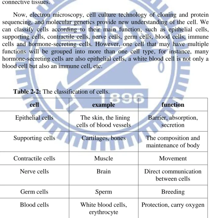
Now, electron microscopy, cell culture technology of cloning and protein sequencing, and molecular genetics provide new understanding of the cell. We can classify cells according to their main function, such as epithelial cells, supporting cells, contractile cells, nerve cells, germ cells, blood cells, immune cells and hormone-secreting cells. However, one cell that may have multiple functions will be grouped into more than one cell type, for instance, many hormone-secreting cells are also epithelial cells, a white blood cell is not only a blood cell but also an immune cell, etc.
Table 2-2: The classification of cells.
cell example function
Epithelial cells The skin, the lining cells of blood vessels
Barrier, absorption, secretion
Supporting cells Cartilages, bones The composition and maintenance of body Contractile cells Muscle Movement
Nerve cells Brain Direct communication between cells Germ cells Sperm Breeding
Immune cells White blood cells, lymphoid tissue
Protection
Hormone secreting cells Thyroid, adrenal Indirect communication between the cells If all the cells in the tissue have the same structure, the tissue is called simple tissue. But most tissues containing different functional cells are called compound tissues. For example, nerve tissue contains supporting cells, immune cells and epithelial cells [5].
2.2.1 Oral mucosal tissue
In a section of healthy oral mucosa, the epithelial tissue showing the hierarchical arrangement includes: the basal-cell layer, the prickle-cell layer and the keratinized layer. The basal-cell is a cubic or a columnar cell in the bottom of the epithelial tissue. Because of the ability of hyperplasia, the nucleus of basal cells that have been coated by some dyes, present a dark color. Above the basal-cell layer, the prickle-cells connect to other prickle-cells by the intercellular bridge. The keratinized layer is in the outermost layer. The keratinized layer is the last level of differentiation in epithelial tissue. According to the keratinized layer, the oral mucosa has resistance to friction.
2.2.2 Oral squamous cell carcinoma
Cancer is a genetic disease, but it is not heritable. It is caused by carcinogenic factors and genetic changes. The normal cycle of its growth has been uncontrolled, leading to an abnormal proliferation. The cancer tissue grows rapidly and can spread to other parts of the body through the blood and lymph. The cancer cells may destroy the organ that has been eroded, and they may be life-threatening.
Oral squamous cell carcinoma (OSCC), also called oral cancer, is an invasive lesion at the oral mucosa. The causes of oral cancer include smoking, drinking, chewing betel nuts, and viral infection. Symptoms include: leukoplakia and erythroplakia on the surface of the oral mucosa, an unexplained tumor, mucosal ulceration that does not heal for a long time, unexplained bleeding and restricted activity of the tongue.
When we observe the lesions of cancer tissue in the oral mucosa, we can determine the changes of type and structure. The changes of type include: increased activity of cell division, the ratio of nucleus and cytoplasm, the number of nuclei chromosomes and the normal space between the cells. The
change of structure means the direction of cell proliferation is uncontrolled. The lamina propria is eroded by the cancerous tissue. In histology, we can classify oral cancer by the degree of differentiation, including well differentiation, moderate differentiation and poor differentiation. The hyper degree of differentiation signifies better healing after surgery.
(a) (b)
Figure 2-2: (a) Well differentiated keratinizing squamous cell carcinoma.
(b) Poorly differentiated keratinizing squamous cell carcinoma.
2.2.3 Process of making sections
When we examine the tissues by light microscope, paraffin embedding is the standard method for making the tissue samples. It is inexpensive, easy to use, and can be done automatically by machine. After the tissues were dissected, the samples were fixed in paraformaldehyde overnight. The samples were dehydrated by placing them in ethanol until the water in the tissue and fixative was removed. The alcohol was then replaced by organic solvents. Finally, the sample was moved into paraffin at the melting point of paraffin. At a normal temperature, the paraffin would solidify, and the sample could be cut into thin slices (2–3μm) without variant.
Since cells are colorless, the sections must be stained before observation by the light microscope. The staining methods include: empirical stains, histochemical stains, enzyme histochemical stains and immunocytochemistry.
stained purple or black, and the cytoplasm is stained red or pink.
2.3 Development of diagnosing cancer using hyperspectral image
2.3.1 Diagnosis of cancer from image
A fluorescent image was produced in the tissue that the light source irradiated. Because imaging provided two-dimensional information, we could easily mark the areas of lesions in the specific excitation wavelength. The fluorescence imaging techniques enabled real-time detection of cancer simple; it is inexpensive and has high sensitivity and specificity. Many studies have been performed using fluorescence imaging [6] to detect cancer in different organs, such as oral cancer and cancer of the lungs [7-12], the bladder [13], the colon [14-20] and the gastrointestinal tract [21-24].
Ina et al. used the laser-scanning fluorescence 351–364nm and 488nm excitation to detect cervical cancer [25]. Due to the essential dye, Mitotracker Orange, they could see the precancer’s cytoplasmic fluorescence in the bottom of the epithelium. They found that the intensity of fluorescence decreased with the development of cancer cells. In this study, only 10 patients were diagnosed, and the sample number was low.
Darren et al. observed the fluorescence images of oral lesions and normal tissues; the images were obtained from 56 patients and 11 normal volunteers [26]. They classified the images as normal and cancer in different fluorescence excitation wavelengths, 365, 380, 405 and 450nm, with the ratio of normalized red-to-green fluorescence and the autofluorescent image. The data were divided into two sets: a training set and a validation set. The training set included: 20% invasive cancer, 28% dysplasia and 52% normal; the validation set included: 14% invasive cancer, 25% dysplasia and 61% normal. With 405nm excitation, the autofluorescent image showed obvious decreased intensity. It had the highest sensitivity (95.9%) and specificity (96.2%) in the training set, and 100% sensitivity and 91.4% specificity in the validation set. They provided a noninvasive and sensitivity tool to diagnose oral cancer. They detected oral lesions using the decrease in autofluorescence images without observing the spectrum.
Catherine et al. used a hand-held device to evaluate oral cancer by location, fluorescence visualization (FV) status, histology and loss of heterozygosity (LOH) [27, 28]. First, they marked a blue line on the surface of the tumor diagnosed by the naked eye. After the light illuminated the tissues, the tissues provided direct visualization, and they marked a green line in the FV loss (FVL) area as the tumor margins. Lastly, they used LOH to analyze the FVL biopsies
from the tumor margins. In a total of 44 patients, the sensitivity was 98% and the specificity was 100%. However, they did not analyze the spectrum of biopsies.
2.3.2 Diagnosis of cancer from spectrum
Diagnosis based on spectrum has the potential to determine the change of material in the cancer cells. The spectrum was classified as the halogen spectrum and the fluorescence spectrum. When the halogen irradiated the section, we recorded the transmittance as the halogen spectrum. When the light source excited the tissue, the fluorescence spectrum was emitted by the tissue. The spectral data were saved to a computer to be analyzed. Many studies have been performed using the spectrum method to distinguish between normal cells and cancer cells, and the method includes: Principal Components Analysis (PCA) [29-31], emission wavelength ratios [32-35], change of intensity [36-40] and artificial neural networks [41, 42].
Irene et al. evaluated low-grade and high-grade dysplasia of Barrett’s esophagus (BE) by fluorescence, scattering properties, and enlargement and crowding of nuclei [43]. They tried to distinguish high-grade dysplasia from low-grade dysplastic and nondysplastic BE, and high-grade and low-grade dysplasia from nondysplastic BE. There were two peaks in the fluorescence with 337nm excitation; the decrease between the two peaks occurring in the 420nm was caused by the absorption of oxyhemoglobin; they combined the corresponding reflectance spectrum to compensate for the decrease.
At 337nm excitation, the line-shape of the spectrum shifted to the right during the progression from nondysplastic to low-grade, to high-grade dysplasia. At 397nm excitation, the increase of intensity was found in the wavelength range 600–750nm. After the corresponding fitting of the reflectance spectrum, the scattering coefficient reflectance spectrum, μs, changed in different grades of dysplastic tissue. They also showed the enlargement of nuclei could be the characteristic, defining diameter > 10μm as enlargement of the nuclei. The analysis combining 3 techniques had a sensitivity of 93% and a specificity of 100%. Their analysis combined the spectrum and image, but the enlargement would be hard to define because of the irregular shape of the nuclei.
Hamed et al. detected cancer by using integral, support vector machines (SVM), spectral standard deviation and the normalized cancer index (NDCI) [44]. The halogen spectrum was normalized to calculate the reflectance using the following equation:
) ( ) ( ) ( ) ( ) ( dark white dark raw I I I I R
(2-1)
where R(λ) is the reflectance value, Iraw(λ) is the raw-data radiance value,
Idark(λ) is the dark current and Iwhite(λ) is the white board radiance. The
wavelength range was 1000–2500nm, and they found the area under the spectral curve was higher in cancer than in normal tissues, while the slopes at 1200–1400nm were lower in cancer tissues. They also used SVM to classify tissue into normal and cancer tissues. They also compared the spectral standard deviation using the following equations, (2–2) in two dimensions and (2–3) in three dimensions: 2 1 2 1 1 1 1 1 2 } ] ) , , ( [ { ) , (
k k k i i i i i j j j j j av R k j i R C j i SD(2-2) 2 1 1 1 1 1 2 1 2 } ] ) , , ( [ { ) , (
i i i i i j j j j j k k k av R k j i R C j i SD(2-3)
where SD was the standard deviation, k was the number of wavelength bands, k1 and k2 were the range of wavelength bands, i and j were spatial coordinates, i1 and j1 were the area size of the predefined neighbor, C was a coefficient, R was the reflectance and Rav was the mean of reflectance. The NDCI was
calculated using the following equation:
4 3 2 2 2 1 2 1 ( ( )) ( ( )) k k k k k k k k d R R d C NDCI(2-4)
where NDCI was the normalized cancer index, C1 and C2 were coefficients, Rk
was the normalized reflectance in wavelength k, d(Rk) was the derivative of Rk ,
k1, k2, k3, and k4 were the wavelength bands. Lastly, the specificity was 88%
using integral, 80% using SVM, 82% using spectral standard deviation and 93% using NDCI. However, they only analyzed the halogen spectrum without the fluorescence that could show the change of biochemistry.
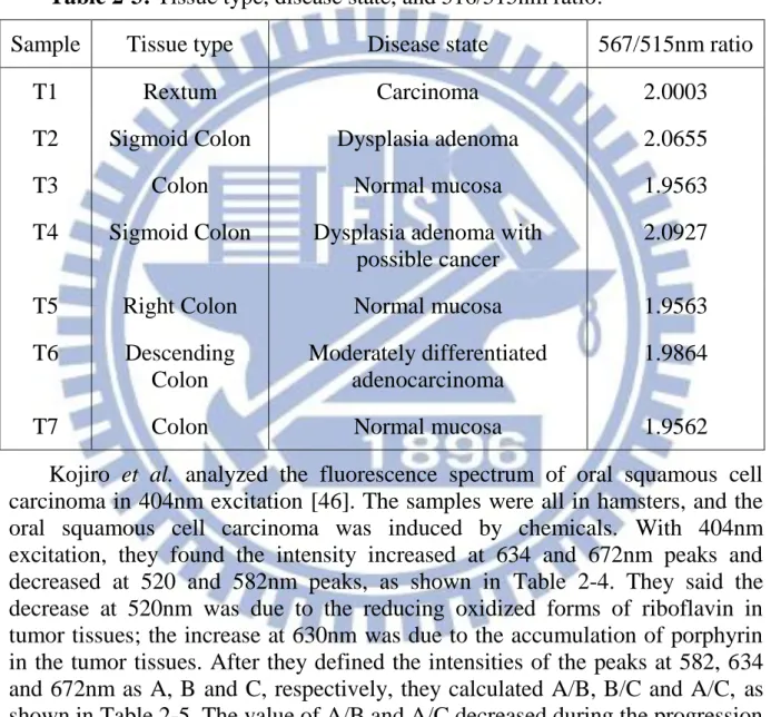
Kevin et al. used the colonoscopy to detect colorectal cancer from two imaging modalities: visible and NIR autofluorescence imaging and hyperspectral reflectance imaging [45]. For normalization, they subtracted the background intensity and divided the corresponding brightfield images. In the autofluorescence imaging, they found that normal tissues emitted more autofluorescence than the cancer tissues in 515nm excitation did, but the normal tissues emitted less autofluorescence than the cancer tissues did in 567nm
excitation. Therefore, they divided the fluorescence intensity at the second peak with 567nm excitation by the fluorescence intensity at the first peak with 515nm excitation to diagnose the colorectal cancer, and the ratio was less than 1.96 in normal mucosa and more than 1.98 in cancer, as shown in Table 2-3. In the hyperspectral reflectance imaging, the result of a total of 7 samples (T1-T7) showed a great correlation between different stages of cancer except for tissue sample T5. However, the number of samples was too low to prove the method was successful.
Table 2-3: Tissue type, disease state, and 516/515nm ratio.
Sample Tissue type Disease state 567/515nm ratio T1 Rextum Carcinoma 2.0003 T2 Sigmoid Colon Dysplasia adenoma 2.0655 T3 Colon Normal mucosa 1.9563 T4 Sigmoid Colon Dysplasia adenoma with
possible cancer
2.0927
T5 Right Colon Normal mucosa 1.9563 T6 Descending
Colon
Moderately differentiated adenocarcinoma
1.9864
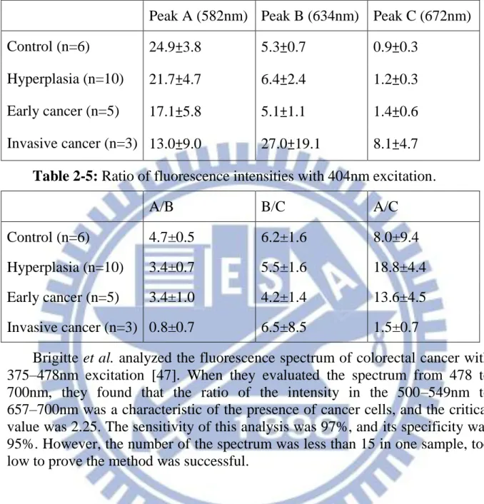
T7 Colon Normal mucosa 1.9562 Kojiro et al. analyzed the fluorescence spectrum of oral squamous cell carcinoma in 404nm excitation [46]. The samples were all in hamsters, and the oral squamous cell carcinoma was induced by chemicals. With 404nm excitation, they found the intensity increased at 634 and 672nm peaks and decreased at 520 and 582nm peaks, as shown in Table 2-4. They said the decrease at 520nm was due to the reducing oxidized forms of riboflavin in tumor tissues; the increase at 630nm was due to the accumulation of porphyrin in the tumor tissues. After they defined the intensities of the peaks at 582, 634 and 672nm as A, B and C, respectively, they calculated A/B, B/C and A/C, as shown in Table 2-5. The value of A/B and A/C decreased during the progression from control to hyperplasia, to early cancer, to invasive cancer.
Table 2-4: Fluorescence intensities with 404nm excitation.
Peak A (582nm) Peak B (634nm) Peak C (672nm) Control (n=6) 24.9±3.8 5.3±0.7 0.9±0.3
Hyperplasia (n=10) 21.7±4.7 6.4±2.4 1.2±0.3 Early cancer (n=5) 17.1±5.8 5.1±1.1 1.4±0.6 Invasive cancer (n=3) 13.0±9.0 27.0±19.1 8.1±4.7
Table 2-5: Ratio of fluorescence intensities with 404nm excitation.
A/B B/C A/C
Control (n=6) 4.7±0.5 6.2±1.6 8.0±9.4 Hyperplasia (n=10) 3.4±0.7 5.5±1.6 18.8±4.4 Early cancer (n=5) 3.4±1.0 4.2±1.4 13.6±4.5 Invasive cancer (n=3) 0.8±0.7 6.5±8.5 1.5±0.7
Brigitte et al. analyzed the fluorescence spectrum of colorectal cancer with 375–478nm excitation [47]. When they evaluated the spectrum from 478 to 700nm, they found that the ratio of the intensity in the 500–549nm to 657–700nm was a characteristic of the presence of cancer cells, and the critical value was 2.25. The sensitivity of this analysis was 97%, and its specificity was 95%. However, the number of the spectrum was less than 15 in one sample, too low to prove the method was successful.
Chapter 3 Methodology
3.1 Embedded Relay Lens Microscopic Hyperspectral
Imaging System (ERL-MHIS)
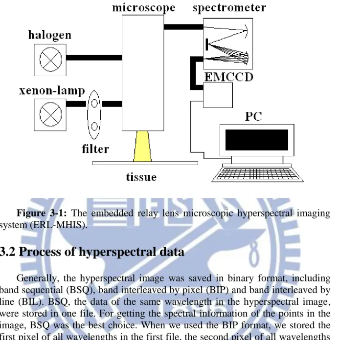
In the measurement process, the system (ERL-MHIS) contained two light sources, one microscope, one spectrometer, EMCCD saving hyperspectral data, and a computer displaying and analyzing the spectrum. The light sources included a halogen spectrum and a fluorescence spectrum with 330–385nm and 470–490nm excitation. The microscope (IX701, Olympus) enlarged the image of the target area on the sample and transferred the image to the spectrometer. Lastly, the halogen spectrum and the fluorescence spectrum were saved as a 1004x1004x1002 three-dimensional matrix by the EMCCD.
The relay lens was between the microscope and the spectrometer. The function of the relay lens was to transfer the image from the object plane to the image plane. By moving the relay lens, we transferred the image without the relative movement between the microscope and the spectrometer.
The hyperspectral data were saved in a personal computer (PC) for analysis. The PC also controlled the ERL-MHIS. A self-written code controlled the motor to move the relay lens for scanning the image of the target area, and set the integration time of EMCCD; the hyperspectral data were also analyzed by the PC.
Figure 3-1: The embedded relay lens microscopic hyperspectral imaging
system (ERL-MHIS).
3.2 Process of hyperspectral data
Generally, the hyperspectral image was saved in binary format, including band sequential (BSQ), band interleaved by pixel (BIP) and band interleaved by line (BIL). BSQ, the data of the same wavelength in the hyperspectral image, were stored in one file. For getting the spectral information of the points in the image, BSQ was the best choice. When we used the BIP format, we stored the first pixel of all wavelengths in the first file, the second pixel of all wavelengths in the second file, the third pixel of all wavelengths in the third file, and so on. According to BIL format, we stored the information of the same split in one image for one file. BIL was the compromise between BSQ and BIP, and it was also the most commonly used.
In the spectra of halogen, we calculated the penetration after removing the light and dark noise. In the halogen, the center of the image had the strongest brightness because of the light source. The light noise was caused by the uneven light source. We calculated the transmittance and removed the dark and light noise using the following equation:
) ( ) ( ) ( ) ( ) ( dark light dark raw I I I I T (3-1)
where T(λ) is the transmittance value, Iraw(λ) is the raw data, Idark(λ) is the
dark noise, and Ilight(λ) is the light noise. In the same way, the hyperspectral
data in the fluorescence needed to have the dark noise removed.
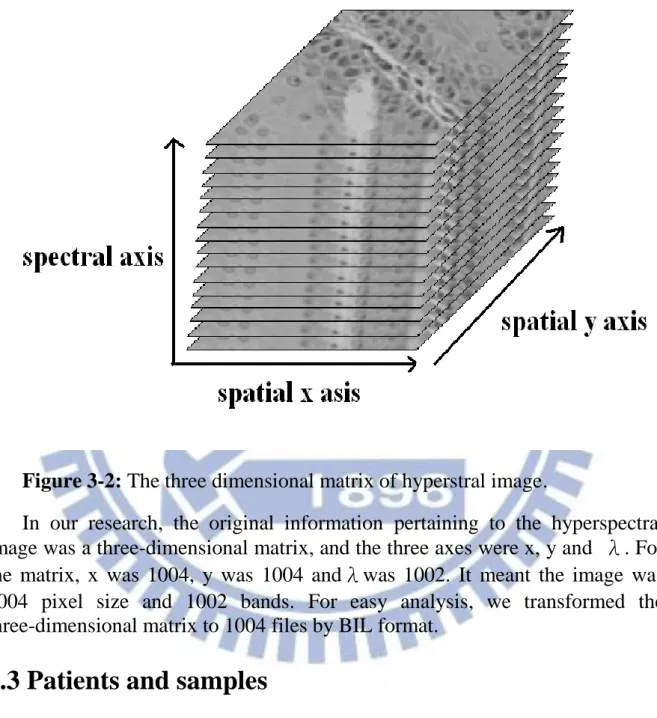
Figure 3-2: The three dimensional matrix of hyperstral image.
In our research, the original information pertaining to the hyperspectral image was a three-dimensional matrix, and the three axes were x, y and λ. For the matrix, x was 1004, y was 1004 andλwas 1002. It meant the image was 1004 pixel size and 1002 bands. For easy analysis, we transformed the three-dimensional matrix to 1004 files by BIL format.
3.3 Patients and samples
We investigated 33 patients in our research, including 32 men and 1 woman: 10 patients with good differentiation, 19 patients with moderate differentiation, and 4 patients with poor differentiation. The biopsy locations involved: 15 sections at the tongue, 6 biopsies at the buccal mucosa, 5 biopsies at the gum, 3 biopsies at the palate, two biopsies at the pyriform sinus, one biopsy at the upper lip, and one biopsy at the bucca and retromolar trigone.
We took two images from each sample: normal and cancer. According to the different light sources: one halogen and two kinds of fluorescent, we had three sets of hyperspectral data in one image, so we had a total of six sets of hyperspectral data on one patient. Because we had the data of light source for only the sample numbers 1~12, we only analyzed the sample numbers 1 to 12 using topology, and analyzed all samples using spectrum.
3.4 Morphological methods for diagnosing oral cancer
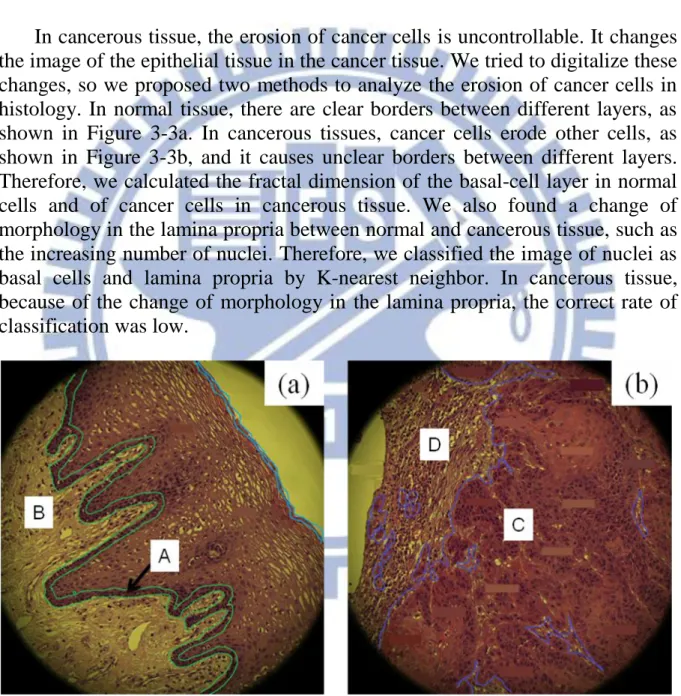
In cancerous tissue, the erosion of cancer cells is uncontrollable. It changes the image of the epithelial tissue in the cancer tissue. We tried to digitalize these changes, so we proposed two methods to analyze the erosion of cancer cells in histology. In normal tissue, there are clear borders between different layers, as shown in Figure 3-3a. In cancerous tissues, cancer cells erode other cells, as shown in Figure 3-3b, and it causes unclear borders between different layers. Therefore, we calculated the fractal dimension of the basal-cell layer in normal cells and of cancer cells in cancerous tissue. We also found a change of morphology in the lamina propria between normal and cancerous tissue, such as the increasing number of nuclei. Therefore, we classified the image of nuclei as basal cells and lamina propria by K-nearest neighbor. In cancerous tissue, because of the change of morphology in the lamina propria, the correct rate of classification was low.
Figure 3-3: The image (a) of normal tissue and (b) cancer tissue. A:
basal-cell layer B: lamina propria in normal tissue C: cancer cells D: lamina propria in cancer tissue.
3.4.1 Fractal Dimension
In the topological dimension, 0 was used for points, 1 for lines, 2 for surface and 3 for volumes. Generally, the value of dimension meant the number of coordinate axis to determine the location of one point for the graphics.
Differing from the topological dimension, the fractal dimension can be a non-integer value. The fractal dimension can be divided into regular and irregular. The dimension of regular fractal, like the Koch curve and the Cantor set, was calculated using the formula (3-2). D was the dimension, m was the number of new sticks and the 1/c signified the scaling factor.
) / 1 ln( ln c m D (3-2)
When we observed the biopsies of cancerous tissue, the cancer cells in the basal-cell layer eroded the lamina propria. If we only leaved the image of the basal-cell layer, we could determine the erosion of the cancer cells by calculating the fractal dimension of the basal-cell layer. The image of the basal-layer in cancerous tissues was more complex than in normal tissues. In other words, the fractal dimension of the basal-cell layer calculated was higher in cancerous tissues than in normal tissues.
We superimposed the image of the hyperspectral data on the wavelength range 500~580nm because the largest difference in the spectral intensity between the basal-cell layer and the lamina propria was there. Then we fuzzified the image superimposed by hyperspectral data in the wavelength range 500~580nm to decrease the effect of nuclei by moving the average. Because the spectral intensity of the basal-cell layer was lower, we tried to use the threshold method to leave the basal-cell layer. The value of the threshold method was decided by the nuclei chosen by hand. Closing was the method to fill the interruption and gap in morphological image processing. We used the closing to remove the small cracks of the basal-cell layer. Lastly, we calculated the fractal dimension by the formula (3–2).
Figure 3-4: The flow chart of analysis by fractal dimension.
3.4.2 Classification by K-Nearest Neighbor
K-nearest Neighbor (KNN) is one of the machine-learning algorithms, and it is instance-based learning. KNN classifies the test data by the closest training data in the feature space. When inputting test data, we calculated the distance between the input and all training data. In the k sets of closest training data, if the majority belonged to a category, the test data also belonged to the category.
Figure 3-5: The flow chart of analysis by KNN classifying.
When we observed the section of cancer tissue, we determined the change of the image in the lamina propria because of the erosion by the cancer cells. Because the morphology of the samples was one by one case, we constructed the training data and used the KNN digitalizing the change of the image in the lamina propria. If we classified the nuclei in the basal-cell layer and lamina
propria by KNN, the correct rate of classification was lower in cancer cells because of the change of the image in the lamina propria by the erosion of the cancer cells. First, we had to establish the training data and test data. To establish the training data, we chose nuclei of the basal-cell layer and of the prickle-cell layer in normal tissue and cancer cells in cancerous tissue, which we labeled as group A. Then we chose some nuclei of the lamina propria, which we labeled as group B. In every coordinate, we got an 11x11 matrix, similar to the size of a cell, and expanded the matrix to the one-dimensional matrix, as in Figure 3-5; we recorded the one-dimensional matrix as training data. To establish the test data, we moved an 11x11 matrix to scan the image. When the intensity of the 5x5 matrix in the center was lower than 80% intensity of the average in the 11x11 matrix, we recorded the 11x11 matrix as a nucleus. After the matrix scanning of the image, we expanded the 11x11 matrix as an one dimensional matrix, as in Figure 3-5, and recorded the one dimensional matrix as test data.
Figure 3-6: Expanding an 11x11 matrix to one dimensional matrix.
According to the training data, we could classify the test data by KNN, and the vector difference between the test data and each set of training data in the feature space was calculated. Lastly, we calculated the correct rate of the lamina propria classified by KNN.
Before analyzing the spectrum, we needed to remove the noise. For instance, the spectrum in halogen dark and light noise needed to be removed; the spectrum in fluorescence only removed the dark noise because there was no data for the light source.
After removing the noise, we marked nuclei in the image of the sample and recorded these coordinates. According to the coordinates chosen by hand, we got the spectrum of these nuclei. We had three methods to analyze these spectral data: four in halogen, four in fluorescence 330~385nm excitation and three in fluorescence 470~490nm excitation.
Figure 3-7: The flow chart of spectral analysis.
3.5.1 Intensity in the specific wavelength range
In some wavelength ranges, the spectral curve showed an obvious characteristic. For searching the specific wavelength range, we compared the spectral intensity every 30nm wavelength range; then we could find the specific wavelength range of the largest difference in intensity. For example, the transmittance of halogen in normal cells was higher than in cancer cells in the 460~480nm, as shown in Figure 3-8a, and we also compared the fluorescence intensity 470~490nm excitation in the wavelength range 540~560nm, as shown in Figure 3-8d.
Fluorescent intensity with 330-385nm excitation. (c) Fluorescent intensity compensated by spline with 330-385nm excitation. (d) Fluorescent intensity with 470-490nm excitation. Red line is normal cells, and blue line is cancer cells. A: the peak in wavelength range 460~480nm. B: the peak in wavelength range 700~710nm. C: the intensity in wavelength range 540~570nm. D: the intensity in wavelength range 680~710nm. E: the maximum of spectral curve. F: the full width at half maximum (FWHM) of spectral curve. G: the peak in wavelength range 540~570nm. H: the FWHM of spectral curve.
3.5.2 Ratio of intensity in two different wavelength ranges
Generally, there were some peaks in the spectral curve. We calculated the ratio of the intensity in different peaks or specific wavelength range. In our research, we calculated the ratio of average halogen transmittance in the range 460~480nm to the 700~710nm.3.5.3 Wavelength of the specific peak
The wavelength of the peak may be different in each spectral curve. In halogen, we compared the wavelength of the maximum in the wavelength 700~710nm. We tried to find the movement of the peak caused by the cancer cells.
3.5.4 Area under spectral curve
By the integration of the spectral curve, we calculated the area under the curve. Before the integration, we needed to normalize the spectral curve. First, we recorded the maximum of the spectral curve, and then we divided the intensity by the maximum. We wanted to diagnose cancer cells by the change of area under the spectral curve.
3.5.5 Maximum of spectral curve compensated by spline
In fluorescence 330~385nm excitation, two peaks occurred in the wavelength range 540~560nm and 700~710nm. The decrease between the peaks that might have been caused by the absorption of hemoglobin, and the spectral curve of fluorescence excitation approximates Gaussian distribution and parabolic[43]. We compensated the decrease and fitted the spectral curve as parabolic by spline. Spline used the slope of the left and right borders to fit aFigure 3-9: Spectrum compensated by Spline. Solid line is fluorescent
spectrum with 330-385nm excitation, dotted line is the spectrum curve compensated by Spline.
3.5.6 Full Width at Half Maximum (FWHM) of spectral
curve
Full width at half maximum (FWHM) refers to the distance between half width of a peak, figure 3-10. After the spectral curve in fluorescence 330~385nm excitation was compensated by spline, we calculated the FWHM of the curve.
Figure 3-10: Full width at half maximum.
3.6 Sensitivity and specificity
Sensitivity means the correct rate of determining the normal cells as normal cells, and specificity means the correct rate of determining the cancer cells as cancer cells. We used the Gaussian distribution to calculate the sensitivity and specificity of our analysis. First, we computed the mean and variance of the result in the analysis; then we could determine the Gaussian distribution using the formula (3-3). μ was the mean, and σ was the variance.
2 2 2 ) ( 2 1 ) ( x e x f (3-3)
By the Gaussian distribution, we determined the critical value of the method, for example, by using the intersection of two curves. We defined the right region as normal tissue and the left region as cancerous tissue. Then we could determine the sensitivity and specificity: sensitivity was the ratio of the area under the solid line and on the left of critical point to the area under the solid line, as shown in Figure 4-9; specificity was the ratio of the area under the dotted line and on the right of critical point to the area under the dotted line, as
Figure 3-11: The Gaussian distribution of the analysis. Red line is normal
cells, and blue line is cancer cells.
Patients with oral cancer Condition Positive Condition Negative Test Outcome Test Outcome Positive True Positive (TP) False Positive (FP) Test Outcome Negative False Negative (FN) True Negative (TN) Sensitivity =TP/(TP+FN) Specificity =TN/(FP+TN)
Chapter 4 Results
4.1 Experiments
This is the flow chart of our experiment. First, we used the hyperspectral scanning system to transfer the optical image of the sample into a hyperspectral matrix. The hyperspectral scanning system includes: a microscope, three light sources, a motor, a relay lens, a spectrometer and an EMCCD. We use the microscope to enlarge the image of the sample. There are three light sources: halogen lamp, fluorescent at 330~385nm excitation and fluorescent at 470~490nm excitation. The motor was used to move the relay lens for scanning the image, and we used the spectrometer to transform the image into the hyperspectral image. Lastly, the EMCCD stored the hyperspectral image in a three-dimensional matrix. The three axes are x, y and λ.
After we transferred the format of hyperspectral data to BIL, we chose the nuclei in the image. These data on nuclei, which were chosen by hand, and used to diagnose cancer cells using the spectral method; they would also serve as the training data in the method of topology. There are two kinds of cancer cell diagnoses: the difference of spectral curves and the change of topology. In the diagnosis by the difference of spectral curves, we have 11 methods to compare the spectrum of normal cells and cancer cells: 4 methods in halogen, 4 in fluorescence 330~385nm excitation and 3 in fluorescence 330~385nm excitation. In the diagnosis of the change in topology, we present two methods: calculating the fractal dimension of the image and the correct rate of the classification by KNN. Lastly, we can plot the Gaussian distribution curve of the value generated by the methods, and calculate the sensitivity and specificity of this method.
Figure 4-1: The flow chart of experiment.
4.2 Morphological analysis of oral cancer
Before our analysis in topology, we needed to remove the light noise. Because we only had the spectrum of light source in samples numbered 1 to 12, we only analyzed the sample numbers 1 to 12 in topology.
4.2.1 Calculation of Fractal Dimension after Threshold
Method
Figure 4-1 shows the result of the threshold method for the samples numbered 1 to 12. After using the threshold method, the basal-cells in normal tissue and the cancer cells in cancerous tissue were set to 1 or white, and the others to 0 or black. The figures on the left in Figure 4-1 are all normal tissue; the figures on the right are cancerous tissue.
We can determine that the threshold method images exnibit a large difference between normal cells and cancer cells. The white area in the normal tissue shows a continuous curve, and the white area in the cancerous tissue shows a discontinuous curve and spreads over the whole image. Table 5-1 shows the fractal dimension of the image after using the threshold method.
According to the Gaussian distribution, we can determine 1.75 as the critical value. If the fractal dimension is lower than 1.75, we identify the image as normal tissue; on the other hand, if the fractal dimension is higher than 1.75, we identify the image as cancerous tissue. The sensitivity is 83.44%, and specificity is 91.46%.
Figure 4-2: After threshold method, the basal cells are white, and the others
are black in the images. The number 1 to 12 of figure means the number of the sample. The label (a) means normal tissue, and the label (b) means cancer tissue.
Table 4-1: The fractal dimension of sample numbered 1 to 12 after
threshold method. Number of patients 1 2 3 4 5 6 7 8 9 10 11 12 (a) Normal cells 1.73 1.73 1.57 1.73 1.24 1.59 1.65 1.66 1.68 1.59 1.66 1.50 (b) Cancer cells 1.90 1.82 1.81 1.67 1.78 1.80 1.85 1.97 1.95 1.89 1.76 1.91
4.2.2 K-nearest Neighbor Classification
According to the training data chosen by hand, we can classify the nuclei as basal-cell and lamina propria. Figure 4-2 shows the result of classification by KNN. A red point means basal-cell and a blue point means lamina propria. Table 4-2 shows the correct rate of classification in lamina propria by KNN. After the calculation of Gaussian distribution, we determined the critical value as 0.76. This means if the correct rate is lower than 0.76, then we indentify the sample as cancerous; conversely, if the correct rate is higher than 0.76, we indentify the sample as normal tissue. The sensitivity is 81.36%, and the specificity is 55.34%.
Figure 4-3: The result of classification by KNN in the sample numbered 1
to 12. The number 1 to 12 of figure means the number of the sample. The label (a) means normal tissue, and the label (b) means cancer tissue.
Table 4-2: The correct rate of classification by KNN in the sample
numbered 1 to 12. Number of patients 1 2 3 4 5 6 7 8 9 10 11 12 (a) Normal cells (%) 80.9 58.3 94.7 87.8 95.0 89.4 86.3 92.2 87.8 91.2 64.9 89.2 (b) Cancer cells (%) 49.8 87.9 73.0 81.6 62.9 80.7 79.9 47.4 100 50.9 70.4 93.6
4.3 Spectral analysis of oral cancer
We chose nuclei in the image as the data for diagnosis of cancer cells by hand, and the number of the data is shown in Table 4-3. Except for sample number 5, we have at least 100 sets of data in one sample. Because we have three light sources, we have to diagnose cancer cells in three kinds of spectrum. We have 11 methods to diagnose cancer cells in spectrum: 4 in halogen, 4 in fluorescence 330~385nm excitation and 3 in fluorescence 470~490nm excitation.
Table 4-3: The number of spectral data.
Number of patient Normal tissue (nuclei) Cancer tissue (nuclei) Number of patient Normal tissue (nuclei) Cancer tissue (nuclei) 1 557 458 18 184 301 2 133 150 19 358 739 3 260 164 20 416 551 4 265 210 21 236 371 5 82 221 22 450 584 6 167 140 23 424 262 7 376 404 24 279 239 8 202 182 25 167 248 9 150 563 26 309 449
10 241 263 27 425 449 11 334 278 28 399 316 12 242 413 29 311 330 13 215 120 30 315 387 14 393 759 31 229 632 15 313 342 32 507 296 16 432 351 33 359 693 17 623 565
4.3.1 Transmitting spectral mode
Figure 5-3 shows the penetration in halogen for the samples numbered 1 to 12. The penetration means we removed the light noise and black noise from the spectral data, and we only have the data of light source in the samples numbered 1 to 12. The maximum of penetration is 1, and the minimum is 0. We have four analytical methods in the spectrum of halogen. Method 1-1 is calculating the penetration in the wavelength range 460~480nm. Method 1-2 is calculating the ratio of the penetration in the range 460~480nm to the penetration in the range 700~710nm. Method 1-3 is calculating the intensity of the peak at 700~710nm.
Table 5-2 shows the specificity of each method in halogen. Except for sample number 2, we can see that methods 1-1 and 1-2 have the highest specificity, the means of which are 87.15 and 86.27, respectively, so we combined methods 1-1 and 1-2 to analyze the spectrum in halogen. If we ignore sample number 2, the mean of specificity is 98.45.
Figure 4-4: The spectral curve of the sample numbered 1 to 12 in halogen.
The red line means normal cells, and blue line means cancer cells. The number means the number of patients. X axis is wavelength (nm), and Y axis is halogen transmittance.
Table 4-4: The correct rate of classification by KNN in the sample number
1 to 12. Number of patient Specificity of method 1-1 (%) Specificity of method 1-2 (%) Specificity of method 1-3 (%) Specificity of method 1-1+1-2 (%) 1 92.5 90.4 43.4 97.4 2 0 0 42.0 0.0 3 99.6 98.9 77.1 100.0 4 98.0 90.4 65.8 100.0 5 95.1 99.7 71.1 100.0 6 92.3 88.4 74.4 92.2 7 83.6 86.6 76.1 97.3 8 96.6 86.4 35.0 100.0 9 99.8 93.7 64.2 100.0 10 99.9 65.2 37.7 100.0 11 94.7 69.9 71.3 96.1 12 96.6 79.4 66.7 100
330~385nm excitation, and Figure 4-6 shows the spectral curves that have been compensated by the spline. We have four methods to compare the normal cells and cancer cells. Method 2-1 compares the ratio of the intensity in the range 540~570nm to the intensity in the range 680~710nm. Method 2-2 calculates the area under the spectral curve that has been normalized by the intensity at 540~570nm. Method 2-3 compares the maximum of the spectral curve that has been compensated by spline. Method 2-4 compares the full width at half maximum (FWHM) of the spectral curve compensated by the spline.
Table 4-5 shows the specificity of the method analyzing the spectrum in the fluorescence 330~385nm excitation. We can see a large difference between the specificity of each sample; it signifies that these analyzing methods are not strong enough.
Figure 4-5: The spectral curves of each sample in fluorescence 330~385nm
excitation. The number of figure means the number of the sample. The red line means normal cells, and blue line means cancer cells. The number means the number of patients. X axis is wavelength (nm), and Y axis is fluorescence intensity (μ w).
Figure 4-6: The spectral curves of each sample which have been
compensated by spline in fluorescence 330~385nm excitation. The number of figure means the number of the sample. The red line means normal cells, and