多人無線近身網路系統

(1)

國立交通大學

電子工程學系電子研究所

博士論文

多人無線近身網路系統

Multiuser Wireless Body Area Networks

研究生：程士恒

指導教授：黃經堯博士

(2)

國立交通大學

電子工程學系電子研究所

博士論文

多人無線近身網路系統

Multiuser Wireless Body Area Networks

研究生：程士恒

指導教授：黃經堯博士

(3)

多人無線近身網路系統

Multiuser Wireless Body Area Networks

研究生：程士恒 Student: ShihHeng Cheng

指導教授：黃經堯博士 Advisor: ChingYao Huang

國立交通大學

電子工程學系電子研究所

博士論文

A Dissertation

Submitted to Department of Electronics Engineering and

Institute of Electronics

College of Electrical and Computer Engineering

National Chiao Tung University

in partial Fulfillment of the Requirements

for the Degree of

Doctor of Philosophy

in

Electronics Engineering

Aug 2012

Hsinchu, Taiwan, Republic of China

(4)

I

多人無線近身網路系統

研究生：程士恒指導教授：黃經堯博士

國立交通大學

電子工程學系電子研究所

摘要

無線近身網路可利用短距離之無線傳輸擷取並傳送人體之重要生理資訊。其目前已被視為實現遠距照護(無遠弗屆醫療照護)之最重要的”最後一公尺”。無線近身網路其架構可以相當多元。透過適當的假設，無線近身網路可被比喻為”個人化之感測網路(personal sensor network)”、”社群用之隨意網路(social ad-hoc network)”、或是”醫療用之網狀網路(medical-specific mesh network)”。也因此目前許多既有之感測、隨意、與網狀網路之技術可用來增進無線近身網路之效能。本研究進一步探討無線近身網路特有之”近身網路間干擾”議題。此議題來自於無線近身網路使用者之移動性。經常性的近身網路移動所導致之彼此重疊或碰撞造成無線節點密度之劇烈變化，因此引發劇烈之近身網路間互相干擾而導致傳輸效能與可靠性之低落。透過建立多近身網路使用者之干擾模型，本研究率先指出近身無線網路之設計挑戰。其包含: 1) 在高密度近身網路情境下，如何同時增進網路使用效能與快速反應因使用者移動性所帶來之拓樸與干擾變化?(以傳統圖學資源分配觀點來看，此兩校能參數互為取捨) 2) 如何在多使用者近身網路中建立洽當之優先權制度?此制度須同時考量感測器類別、

(5)

II

使用者狀態、與緊急事件總類等之個別差異性。 3)如何在分散式網路的架構下實現以上需求? 在本論文中，我們針對各議題做深入討論並提供其個別的解決方案，包含隨機非完整著色法(Random Incomplete Coloring)用來最大化無線近身網路資源分配之速度與頻道利用效率與隨機資源競爭(RACOON)演算法用來實作分散式近身網路之優先權制度。其個別效能探討將搭配相關理論模型與電腦實驗。

關鍵字：無線近身網路，感測器，低功耗，頻道效益，品質服務(QoS)，媒體接 取控制，資源分配，著色理論。

(6)

III

Multiuser Wireless Body Area Networks

Student: ShihHeng Cheng Advisor: Dr. ChingYao Huang

Department of Electronics Engineering

and

Institute of Electronics

National Chiao Tung University

Abstract

Wireless Body Area Network (WBAN) is designed to retrieve important body signals through short range wireless technology in charge of the “last meter” of ubiquitous healthcare. With proper assumptions of network architecture, WBAN can be regarded as a “personal sensor network”, a “social ad-hoc network”, or a “medical-specific mesh network”. Based on the experiences of these well-known wireless technologies (sensor, ad-hoc, and mesh networks), this study further discusses and puts more focus on effects of “inter-WBAN interference.” This multi-WBAN-specific issue is caused by the mobility of WBAN users. When WBANs are moved with users, they frequently encounter and overlap with each other. These WBAN-overlaps lead to dramatic changes of sensor density and hence creates dynamic mutual interferences between WBANs. Through establishing interference models of multiuser WBANs, this study first identifies design challenges under the inter-WBAN interference. Primary challenges include 1) simultaneously improving channel efficiency in high density WBAN while maintaining fast response time to rapid WBAN topology changes (these two performance indexes are tradeoffs in term of traditional scheduling theory), 2) Constructing the proper priority scheme for multiuser

(7)

IV

WBAN which can simultaneously satisfy priority requirements from sensor types, user conditions, and emergency-handling points of views, and 3) solving these problems in distributed WBAN systems. This study will discuss above issues in separate chapters. Corresponding solutions, Random Incomplete Coloring (RIC) and RACOON algorithms that solve speed-efficiency trade-offs of traditional coloring and WBAN-specific priority schemes, respectively, will be introduced. Improvement of related performance indexes will be carefully verified by proper analytical models and experiments.

Keywords: Wireless Body Area Network, Sensors, Low Power, Channel Efficiency, Quality of Service (QoS), Medium Access Control, Resource Scheduling, Graph Coloring.

(8)

V

Acknowledgements

I would like to dedicate this work to my love, Karen, and my family.

I want to thank Prof. ChingYao Huang for all his valuable advices and supports of this study. I also want to thank National Chiao-Tung University (NCTU) and WanFang Hospital’s U-PHI project team members who inspired me to combine medical and tele-healthcare experiences in my work. I want to specially thank Prof. Hung-Lin Fu for his advices to the math models constructed in this study. Finally, I appreciate all important suggestions from my dissertation committees that have helped complete this work.

(9)

VI

List of Tables

(12)

IX

List of Figures

Fig. 1-1 Wireless body area networks (WBAN) ... 2

Fig. 1-2 General WBAN architectures ... 3

Fig. 2-1 Wireless body area networks (WBAN) (a) Topology of WBAN (b) Traffic load of WBAN ... 8

Fig. 2-2 Power consumption of beacon, slotted CSMA/CA, and Hybrid modes. ... 15

Fig. 2-3 Maximum G (Number of WBANs) ... 15

Fig. 2-4 Hybrid access mode ... 16

Fig. 3-2 Oriented and non-oriented colorings (Pri-arts) ... 22

Fig. 3-3 CPN-based inter-WBAN scheduling (IWS) ... 24

Fig. 3-4 Random incomplete coloring ... 27

Fig. 3-5 Random incomplete coloring ... 29

Fig. 3-6 Rounds per coloring cycle (Rpc) of RIC and INC-only ... 37

Fig. 3-7 Vertices per color (Vpc) of analytical model and simulations of RIC 38 Fig. 3-8 Vertices per color (Vpc) of RIC and complete colorings ... 39

Fig. 3-9 Superframe for coloring-based IWS ... 41

Fig. 3-10 Transmission per Slot (Tps) of IWS (ignoring ill-scheduling) ... 44

Fig. 3-11 System throughput of IWS with the Fixed-p Model ... 45

Fig. 4-1 Wireless Body Area Network ... 48

Fig. 4-2 CPN-based resource allocation of RACOON ... 54

Fig. 4-3 Probing-based interference detection ... 56

Fig. 4-4 Random Contention-based Inter-CPN negotiation of RACOON ... 57

Fig. 4-5 Bandwidth control flow of inter-CPN negotiation in RACOON ... 60

Fig. 4-6 Multi-queue scheduler of intra-WBAN scheduling ... 61

Fig. 4-7 Packet latency of vital signals in high and low priority WBANs ... 64

Fig. 4-8 Packet Latency with RACOON and BodyQoS ... 65

Fig. 4-9 Packet collisions with RACOON and BodyQoS controls ... 66

Fig. 4-10 Energy consumption of WSN with RACOON and BodyQos ... 67

(13)

1

Chapter 1 Introduction of Multiuser WBANs

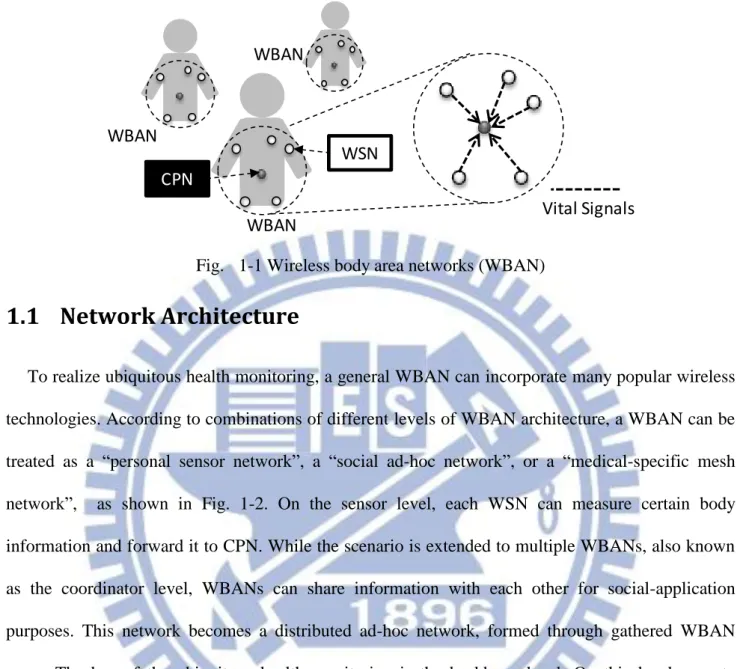
Wireless Body Area Network (WBAN) is a short range communication (3~5 meters) which realizes ubiquitous health monitoring by breaking the wire-line limitation of traditional near/inner body signal measurements. WBAN bridges these “last meter” vital signals with hospital or clinics for further diagnosis and health tracking [1, 2]. As illustrated in Fig. 1-1, a single WBAN can be regarded as a “personal sensor network,” formed by a group of wireless sensor nodes (WSNs) and a central processing node (CPN) that collects various vital signals from these WSNs. However, different from traditional sensor networks focused on static or low mobility scenarios [3], a WBAN has a higher moving speed1 and more frequent topology changes due to user movement [2]. The moving topology of multiple WBANs is similar to that of mobile ad hoc networks (MANETs) [4], but with group-based rather than node-based movement. The “high mobility” and “group-based movement” differ the WBAN from a sensor network and a MANET. These properties of WBAN create a new research topic of inter-WBAN interaction, which includes new inter-WBAN interference and quality of services (QoS) issues. Hence, a WBAN-specific medium access control (MAC) is required. Before discussing design challenges of WBAN MAC, the network architecture of WBAN is introduced to specifically define the scope of this study.

1 A WBAN has “notable mobility” by considering its short transmission range (3~5meters) as compared with human moving speed (meters per second when walking or running).

(14)

2 Vital Signals CPN WSN WBAN WBAN WBAN

Fig. 1-1 Wireless body area networks (WBAN)

1.1 Network Architecture

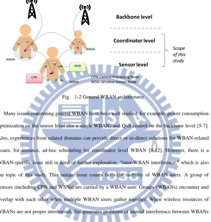
To realize ubiquitous health monitoring, a general WBAN can incorporate many popular wireless technologies. According to combinations of different levels of WBAN architecture, a WBAN can be treated as a “personal sensor network”, a “social ad-hoc network”, or a “medical-specific mesh network”, as shown in Fig. 1-2. On the sensor level, each WSN can measure certain body information and forward it to CPN. While the scenario is extended to multiple WBANs, also known as the coordinator level, WBANs can share information with each other for social-application purposes. This network becomes a distributed ad-hoc network, formed through gathered WBAN users. The key of the ubiquitous health monitoring is the backbone level. On this level, remote hospitals or tele-healthcare center can receive the body signals collected by CPN through cellule systems.

(15)

3 CPN WSN WBAN WBAN WBAN Backbone level Coordinator level Sensor level

CPN: Central Processing Node WSN: Wireless Sensor Node

Scope of this study

Fig. 1-2 General WBAN architectures

Many issues concerning general WBAN have been well studied, for example, power consumption optimization on the sensor level (for a single WBAN) and QoS control on the backbone level [5-7]. Also, experiences from related domains can provide direct or in-direct solutions for WBAN-related issues, for instance, ad-hoc scheduling for coordinator level WBAN [8-12]. However, there is a WBAN-specific issue still in need of further exploration, “inter-WBAN interference,” which is also the topic of this study. This unique issue comes from the mobility of WBAN users. A group of sensors (including CPN and WSNs) are carried by a WBAN user. Groups (WBANs) encounter and overlap with each other when multiple WBAN users gather together. When wireless resources of WBANs are not proper interleaved, this generates problems of mutual interference between WBANs (sensor groups). To analyze this issue, this study focuses on the architecture in the coordinator and sensor levels with following assumptions:

 WBANs are fully distributed systems – There are no higher advanced coordinator than WBANs. Even if it were possible to share information between WBANs through a backbone system, due to the backbone latency, Backbone system may not be able to timely exchange

(16)

4

real-time information like mutual locations, network loading, and priorities between WBANs. These information are important for instant resource allocation between WBANs. Therefore, this study assumes that each WBAN can only share data with its neighbors that are within its communication range. Each WBAN performs this communication individually.

 Each WBAN has a simple-star topology – Each WBAN is formed by a CPN and a group of WSNs. Usually, WSNs are designed to have meters transmission range, which is larger than the normal size of a human body. Hence, this study assumes each CPN can directly access each WSN in a one-hope communication.

 CPN-based resource scheduling – This study adopts a CPN-based scheduling due to the imbalanced CPN/WSN architecture of a simple star (Fig. 1-1). In a single WBAN, the CPN plays the role of the master and the WSNs are the slaves. The CPN manages the join, leave, and functional-control of the WSNs. In contrast, WSNs are passive devices, which are designed to retrieve specific vital signals such as blood pressure or electrocardiograms (ECG) and forward them to the CPN. Additionally, a CPN is usually embedded in personal devices such as cellular phones or PDAs with larger and rechargeable batteries. Dissimilarly , a WSN is expected to be light weighted (small battery) and even non-rechargeable for certain implantable applications. These two unbalanced features suggest shifting power-consuming network controls from WSNs to the CPN. Therefore, for the inter WBAN scheduling. CPN represents its WBAN and negotiates wireless resources between WBANs. And then, for the intra WBAN scheduling, CPNs centrally allocates the wireless resources (reserved in the inter WBAN negotiation) to its WSNs based on their traffic loading and QoS requirements.

(17)

5

As a result, WSNs only function when receiving commands from CPNs and transmitting data in its allocated wireless resource to minimize power consumptions.

1.2 Design Challenges of Multi-User WBAN MAC

As mentioned, inter WBAN interference comes from the mobility of WBAN users. WBAN densities can vary when WBAN users are alone or in a crowded place. Mutual interferences between WBANs might seriously impact the channel efficiency in high density WBANs. This is the reason that IEEE 802.15 TG6, the standard task group of WBAN, requires that the WBAN protocol support at least the sensor density: 60 sensors in a 6 m space [13]. Furthermore, densities could change very 3 3 rapidly in certain scenarios, before and after entering a crowded elevator for example. Therefore, improvements on maintaining high channel efficiency in crowded WBANs and conducting short response time to the density change of WBANs are major design targets of WBAN MAC. However, these two performance indexes are tradeoffs according to traditional coloring theory, an important theory for resource scheduling, and will thus be discussed in chapter 3).

Mutual interference also leads to complex priority issues in WBAN QoS designs. In each WBAN, WSNs may have difference priorities according to signals they collect. For example, the priority of ECG sensors might require higher priority than that of temperature sensors, since ECG sensor directly respond to life-threatening instances. Also, priorities of sensors may dynamically increase when abnormal signals are detected. This can ensure immediate triggering of related emergency procedure. In addition, priority definitions may various depending on the status of WBAN users. For example, the priority of the temperature of a user in fever may require higher priority than that of a healthy user. As a result, complex priority requirement is another major design challenge for multiuser WBAN MAC.

(18)

6

In this study, the impact of inter-WBAN interference will be first evaluated in chapter 2. Analytical throughput and energy consumption models are provided to point out the key of performance degradation. Chapter 3 further considers the rapid topology change of WBAN and discusses the tradeoff between fast-response-time and channel-efficiency of WBAN resource scheduling. A possible relaxed coloring method is also proposed to skip this tradeoff limitation. Based on the MAC design from chapter 3, solutions for complex priority control of WBAN QoS is further suggested in chapter 4. Finally, chapter 5 summarizes concluding remarks in this WBAN research.

(19)

7

Chapter 2 Analysis of multiuser interference

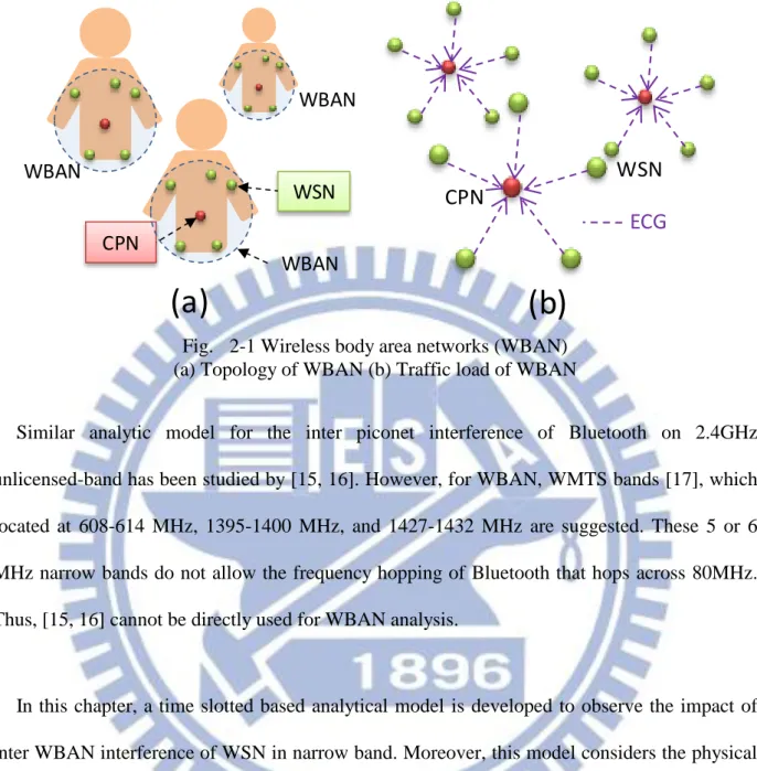
The reason of power consumption may comes from many reasons including overhearing, idle listening, collision, control message, which are identified in [14]. However, for WBAN, collision is the major source of power waste due to its imbalanced network structure. A WBAN consists of a central processing node (CPN) and several wireless sensor nodes (WSNs), which is illustrated in Fig. 2-1(a). For the general WBAN scenario, vital signal collection, the major traffic loading comes from the uplink vital signals (Fig. 2-1(b)), which implies that WSN is the major transmitter and CPN is the major transmitter. Thus, for WSN, collision is the major source of power consumption. For CPN, overhearing and idle listening are the major sources. The energy spent on control messages can be ignored by assuming that data volume is much larger than the control message. However, the importance of low power CPN is lower than WSN for the reason that CPN, which will most likely be embedded in smart phone or equipments with plug-in power, usually has larger batter than WSN. As a result, how to solve the collision problem of WSN becomes the major issue of low power WBAN.

(20)

8 CPN WSN WBAN WBAN WBAN

(a)

CPN

WSN

ECG

(b)

Fig. 2-1 Wireless body area networks (WBAN) (a) Topology of WBAN (b) Traffic load of WBAN

Similar analytic model for the inter piconet interference of Bluetooth on 2.4GHz unlicensed-band has been studied by [15, 16]. However, for WBAN, WMTS bands [17], which located at 608-614 MHz, 1395-1400 MHz, and 1427-1432 MHz are suggested. These 5 or 6 MHz narrow bands do not allow the frequency hopping of Bluetooth that hops across 80MHz. Thus, [15, 16] cannot be directly used for WBAN analysis.

In this chapter, a time slotted based analytical model is developed to observe the impact of inter WBAN interference of WSN in narrow band. Moreover, this model considers the physical transmission rate and the application data rate, which is expected to provide more realistic mode for WBAN analysis.

(21)

9

2.1 WBAN Performance Model of Beacon and Slotted CSMA/CA

Modes

To evaluate the performance impact from the inter WBAN collision, two classic medium access methods, Beacon and carrier sense multiple access and collision avoidance (CSMA/CA), are chosen. The tradeoffs between adopting the deterministic (Beacon) and non-deterministic (CSMA/CA) scheduling are expected to be observed through the modeling of the throughput and the power consumption of these two modes. Beacon and CSMA/CA modes have different approaches to handle the WBAN collisions. For Beacon mode, the transmission time of different nodes in the same network are interleaved to avoid the intra network collision (IANC) by using the Beacon message. However, without knowing the transmission schedule of neighbor WBANs, inter WBAN collision (IRNC) cannot be avoided. Different from Beacon mode, CSMA/CA can avoid IANC and IRNC by using detection-backoff-transmission procedure. If a node senses a busy channel, it performs the backoff-detection procedure until an idle channel is available and thus collisions could be avoided. However, the waste of transmission opportunity due to the random backoff might be the potential problem that limits the throughput.

The power model of WBAN considers a fully connected network with G simple-star WBANs and N WSNs per WBAN. As for the WBAN traffic model, 8kbps ECG traffic is continuously transmitted from each WSN to CPN. The power model of WSN can be formulated by two steps. First, we calculate the energy consumption per packet for Beacon and slotted CSMA/CA modes. Next, by calculating the transmission time per packet, the average power consumption in time can be obtained.

(22)

10

We first define an access period L(slots) to fairly compare the performance of these two modes. In both modes, each node attempts to select one slot to transmit a packet within the access period L. For the Beacon mode, one access period equals to one Beacon period. By using the Beacon message, CPN can assign one transmission slot for each WSN within the Beacon period. As for slotted CSMA/CA, one access period equals to one contention period. Each WSN will contend for one slot within the contention period of L slots.

Slotted CSMA-CA might need more than one attempts and backoff mechanisms to avoid collision. Each node repeatedly detects channel until the idle channel exists. If the channel is busy, the node backoffs to the next contention period. In this scenario, the energy spent for one packet,

J

_CS, is expressed as:

_ cos CS

PKT

CS J JCS t ATTEMPs

J

   (2-1)

where

J

_PKT is the energy spent on packet transmission.

J

_CS_{_ cos}_t is the extra energy cost for the channel detection. ATTEMPs is the expectation number of contentions before a successful CS transmission in CSMA/CA. ATTEMPsCS relates to the probability of intra and inter network collisions,

P

_IANC and

P

_IRNC respectively, are expressed as:











1 1 1 1 1 _,1 1 1 ₁ i CS IRNC IANC IRNC IANC

i IRNC IANC ATTEMPs i P P P P G GN P P L  _                  _



(2-2)

(23)

11

where i is the number of attempts. The attempt is repeated until the idle channel exists. The

probability of intra network collision, P_IANC, equals to

1 1 1 1 N L         

  by assuming each node

uniformly competes with the rest N1 nodes in the same WBAN during the period of L. P_IANC can be further approximated as N 1

L 

when L 1. For the same reason, P_IRNC equals to

( 1) 1 1 1 G N L            and is approximated to (G 1)N L  as L 1.

Different from slotted CSMA/CA, the Beacon mode resolves the intra network collision (IANC) by allocating separated time slots for different WSNs. In this case, the cost in the Beacon mode,

_ cos

BCN t

J , is the listening cost. We assume the Beacon uniformly assigns the slots for each WSN within Beacon period. Collision happens only when two or more nodes from different networks are assigned to the same slot. P_IRNC in the Beacon mode is the same as that in CSMA/CA and equals to

(G 1)N L 

. The energy consumption per packet under the Beacon mode J_BCN can be expressed as:





_ cos 1 _ cos ₁ _ cos ( ) ( ) 1 1 ( ) ,1 , . ( 1) 1 BCN PKT BCN t BCN i PKT BCN t _i IRNC IRNC PKT BCN t J J J ATTEMPs J J i P P J J G N G N L  _             _     



. (2-3)

Next, we want to relate the J_BCN and J_CS with the throughput of WSN. We assume all packets have the same fixed size. Thus the throughput can be defined as the packets successfully transmitted per slot time. For instance, in Beacon mode, ATTEMPs_BCN implies the number of transmission attempts per packet. Thus, the throughput of WSN in the Beacon mode can be expressed as:

(24)

12 1 1 1 ( 1) 1 1 1 4 ( 1) 2 1 ( 1) 4 BCN BCN BCN BCN BCN Tp L ATTEMPs L G N L Tp G N L Tp Tp G N      _            (2-4)

Equation (2-4) shows the tradeoff between throughput TpBCN and (G1)N. As shown, if there is a minimum throughput requirement, the maximum number of G implying the number of WBAN users is limited. We found that L has two possible solutions. The throughput in (2-4) is supposed to be higher for small L, which means WSN attempts to transmit more often. However, the collision also increases with the increase of the transmission rate. This can be proved from P_IRNC in (2-2) with small L . Collision decreases the number of successful transmission and makes the throughput lower than expected. From (2-3), larger L has smaller energy consumption. This implies that for given throughput, large L is a better choice than small L because large L can save more energy and reduce the collision rate. With large L, J_BCN can be rewritten as:

_ cos ( ) 1 1 4 ( 1) 1 1 4 ( 1) 2 ( 1) BCN PKT BCN t BCN BCN BCN J J J Tp G N Tp G N Tp G N        _ _        (2-5)

(25)

13 _ cos 1 1 4 ( 1) 1 1 4 ( 1) 2 ( 1) 1 1 1 1 1 1 4 ( 1) 2 1 ( 1) 4 CS PKT BCN t CS CS CS CS CS CS CS J J J Tp GN Tp GN Tp GN Tp L GN L Tp GN L Tp Tp GN    _ _ _  _ _           _            (2-6)

In the second step, the average power consumption can also be computed by dividing the energy per packet by the transmission time per packet. We assume that the energy only consumed when WSN in TX and RX periods in both modes. During the OFF period, WSN goes to sleep and consumes no power. The power consumption in TX and RX modes is denoted as W_ON. Thus, the average power of WSN in Beacon mode, W_BCN, is expressed as:

_ cos _ cos _ cos _ _ ( ) 2 ( ) 1 1 4 ( 1) BCN BCN BCN BCN t PKT ON ON PKT BCN t BCN PHY PHY PKT PKT BCN PHY PHY bps PKT BCN t PHY ON PKT bps PHY J W

L ATTEMPs Time per slot

B B W W J J ATTEMPs R R B B L ATTEMPs L R R Tp B B R W B Tp G N R            _ _          (2-7)

(26)

14

Where Tp_bps (bits/s) is the throughput. B_PKT(bits) and B_BCN_{_ cos}_t are the size of data and Beacon packets respectively. R_PHY(bits/s) is the minimum transmission rate of physical layer that allows a packet to be transmitted per slot. Following similar steps, W_CS can be expressed as:

_ cos 2 2 ( ) 1 1 4 ( 1) 2 ( 1) 1 1 4 ( 1) bps PKT CS t PHY PKT bps PHY CS _ON bps PHY bps PHY Tp B B R B Tp GN R W W Tp R GN Tp GN R    _                   _ _      _ _{ }    _ _      _ _   _ _    (2-8)

2.2 Analysis and Hybrid Mode

2.2.A

Power consumption of WBAN

We found that both Beacon and slotted CSMA/CA modes have their own advantage. In Fig. 2-2,

N is fixed to evaluate the power consumption of WSN with various number of WBAN groups. CSMA/CA mode has lower power consumption than Beacon mode (Fig. 2-2) because CSMA/CA adopts the channel detection to avoid collision. The cost of channel detection is lower than the packet collision because the detection will not listen to the channel for whole time of packet receiving. However, with given throughput requirement, CSMA/CA supports less number of WBAN groups treated as overall WBAN user capacity than Beacon mode (Fig. 2-3). The body signals monitoring may fail or stop for the insufficient throughput of WSN when the number of user is higher than the limit. Although CSMA/CA has the lowest power consumption, it might fail to meet high user

(27)

15

capacity criterion. To provide both high user capacity and low power WBAN, a new access method should be developed. 0.0320 0.0340 0.0360 0.0380 0.0400 0.0420 0.0440 1 2 4 8 16 32 P o w er o f W SN (mW ) G (Number of WBANs) BCN_N=5 CS_N=5 Hyd_N=5 BCN_N=20 CS_N=20 Hyd_N=20

Fig. 2-2 Power consumption of beacon, slotted CSMA/CA, and Hybrid modes.

/ _ cos 10 , 8 , 0.2 , 2.5 . ON bps BCN CS t PHY W  mW Tp  kbps B  kb R  Mbps 0 2 4 6 8 10 12 14 16 18 Ma xi mu m G (N u mb er o f W BA N s)

Fig. 2-3 Maximum G (Number of WBANs)

8 , 8 , 2.5 .

PKT bps PHY

(28)

16

2.2.B

Hybrid access mode

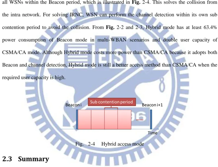
The proposed Hybrid mode adopting both Beacon and channel detection achieves high user capacity and low power. In the Hybrid mode, Beacon is used to solve the IANC and channel detection is used to handle the IRNC. The Beacon assigns non-overlapped sub contention periods for all WSNs within the Beacon period, which is illustrated in Fig. 2-4. This solves the collision from the intra network. For solving IRNC, WSN can perform the channel detection within its own sub contention period to avoid the collision. From Fig. 2-2 and 2-3, Hybrid mode has at least 63.4% power consumption of Beacon mode in multi-WBAN scenarios and double user capacity of CSMA/CA mode. Although Hybrid mode costs more power than CSMA/CA because it adopts both Beacon and channel detection, Hybrid mode is still a better access method than CSMA/CA when the required user capacity is high.

Time Beacon i Sub contention period Beacon i+1

Fig. 2-4 Hybrid access mode

2.3 Summary

In this chapter, we have provided an analytical model to analyze the power consumption and capacity limits of different medium access control schemes in mobile WBAN. Results show that neither the Beacon-based nor detection-based access scheme can effectively support both the low power consumption and high capacity (in terms of WSN nodes) simultaneously. A hybrid mode

(29)

17

proposed in this chapter can provide higher capacity while the power consumption is still well managed. This implies a mixed method may be a better solution for WBAN MAC.

(30)

18

Chapter 3 Distributed multiuser resource scheduling

However, unlike a sensor network focused on static or low mobility scenarios [3], a WBAN has a higher moving speed and more frequent topology changes due to user movement [2]. The moving topology of multiple WBANs is similar to that of mobile ad hoc networks (MANETs) [4], but with group-based rather than node-based movement. The “high mobility” and “group-based movement” make the WBAN neither equivalent to a sensor network nor to a MANET. A WBAN thus has a high chance of encountering other WBANs, which creates new issues of inter-WBAN scheduling (IWS). Corresponding discussions [16, 18-21] have just been opened and comprehensive studies are still required.

Distributed interference-avoidance scheduling of wireless networks can be modeled by the notion of distributed graph coloring, which is commonly adopted in sensor networks or MANET [9, 22, 23]. Network topology is modeled as a graph G( , )V E . The vertices V of G represent the wireless nodes; the edges E of G represent radio resource conflicts between mutually-interfering node pairs; the color set C in a coloring of G represents the set of distinct resource units (can be time slots, frequency bands, or code sequences). A complete vertex k-coloring of a graph G is a mapping V G( )C, where C k, such that adjacent vertices receive distinct colors. Thus, interference between wireless nodes can be avoided by mapping different colors (resource units) to adjacent vertices (mutually-interfering nodes). A standard message-passing model is adopted in this study. To negotiate the color mapping between vertices, they can have a two-way message exchange

(31)

19

with its adjacent vertices. We assume the system is fully synchronous. In other words, all vertices start their coloring algorithms at the same time and execute each step of the algorithm simultaneously. Other terminologies in graph theory refer to [24]. The chromatic number ( )G is defined as the minimum k used to completely color graph G; N v( ) is defined as the set of adjacent vertices of vertex v ; the maximum degree ( )G is defined as the maximum d v( ) and v V G ( ), where vertex degree d v( ) N v( ).

Two basic requirements of IWS are: (i) fast convergence and (ii) high channel utilization. In the case of a WBAN user walking on a sidewalk, network topology changes frequently when the user keeps encountering other WBAN users. Therefore, a quick IWS that rapidly detects and responds to every topology change is expected, which could adopt the quick 1 ( )G coloring for MANET [25]. Also, IEEE 802.15 TG6, the standard task group of WBAN, requires that the WBAN protocol should support at least the sensor density: 60 sensors in a _{6 m space [13]. Such dense WBANs create a}3 3

high probability of mutual interference. It can significantly decrease the number of coexisting WBAN users due to poor channel utilization [19]. Thus, high channel-utilization IWS is also required, which could adopt an optimal spatial-reuse coloring for dense sensor networks [22]. Optimal spatial-reuse implies the maximal number of sensors that access the wireless channel at the same time.

However, references [26-28] show that quick (low time-complexity) coloring and optimal spatial-reuse coloring are trade-offs which cannot be simultaneously achieved with conventional complete coloring. Optimal spatial-reuse coloring uses a minimum number of colors, the chromatic number ( )G , to color a graph. The fewer colors used, the more there is color-reuse among vertices. It implies more wireless nodes can simultaneously transmit packets using the same resource unit, that is, the system has higher spatial-reuse and channel-utilization. However, completely color a graph by

(32)

20

using ( )G colors is known to be NP-complete. The fastest ( )G -coloring so far still needs time-complexity _O(2n_nO(1))_{[26]. Nevertheless, study [27] indicates that time-complexity can be} significantly reduced to O(log )n if colors are increased to 1 ( )G (sacrificing spatial reuse) and

distributed coloring techniques are adopted. 1 ( )G ( )G is known as Brooks’ theorem, which is a loose upper bound for ( )G . A recent work [29] adopts a similar 1 ( )G coloring method. It guarantees not only O(log )n time-complexity but also O(log )n bit complexity, which is the amount of information exchanged between vertices during coloring. Low-bit-complexity of a coloring algorithm makes it applicable to low-computing-power applications, such as sensor networks. Although [28] further decreases the time complexity from O(log )n to2 O( log )n by applying vertex priority, 1 ( )G colors are still required. As a result, neither ( )G [26] nor

1 ( )G -coloring [27, 28] may be directly applied to IWS due to their high time-complexity and low spatial-reuse, respectively.

This chapter proposes Random Incomplete Coloring (RIC) to realize quick and high spatial-reuse IWS. RIC consists of 1) a proposed random-value coloring method and 2) an incomplete-coloring approach. The random-value coloring method is a technique which realizes prioritized vertex coloring [28] (so-called oriented coloring) and will be proven to have a low time-complexity3

(2ln ) 2

W n

O e_ _, which is even lower than [28] . Besides, for high spatial-reuse coloring, conventional complete coloring using ( )G colors is known as the solution for optimal spatial-reuse. Surprisingly, for designs of wireless resource scheduling, this study found that higher spatial-reuse (on average) than that of ( )G coloring is possible if partial vertices are allowed to be uncolored

2

(33)

21

and only k( )G colors are used. In wireless networks, we observe that uncolored vertices imply wireless nodes with no transmission, which do not interfere each other. Hence, following the nature of wireless communication, there is no conflict between adjacent uncolored vertices (or with the special color: no color). Based on this fact, we can color a subgraph of graph G. This subgraph is constructed using vertices, excluding uncolored ones. Clearly, it is possible to use less colors for the subgraph. For convience, we name this kind of coloring “incomplete” coloring. The proposed Random Incomplete Coloring (RIC) will be implemented as an inter WBAN scheduling protocol with a TDMA framing structure, a common structure used in sensor or body area networks [2], to test its convergence speed and spatial reuse in various mobile WBAN scenarios.

The rest of this chapter is organized as follows: section 3.1 introduces the details of related works and the problem formulation. Section 3.2 reveals the proposed RIC algorithm. The corresponding analytical models of RIC are provided in section 3.3. Section 3.4 presents the simulation settings and results. Section 3.5 concludes this chapter.

3.1 Related Works and the WBAN System Model

3.1.A Oriented and Non-oriented Coloring

Oriented vertex coloring [28] is a distributed coloring technique that utilizes predefined edge orientation (vertex priority) to improve the coloring speed of (non-oriented) random vertex coloring [27] from O(log )n to O( log )n . Here we refer to [27] as non-oriented vertex coloring to distinguish [28] from [27]. The major difference between oriented and non-oriented coloring is the

3 _{W x}_{( )}

(34)

22

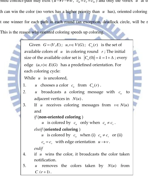
manner of solving color conflicts, as shown in Fig. 3-2 Step 3. For non-oriented coloring, when color conflict c_uc_v happens to vertices pair ( , )u v , both vertices give up that color and re-choose new colors for the color contention in the next coloring round. In contrast, oriented coloring tries to force the vertex that has a higher priority (having an outward edge orientation) to win the color. Although an oriented conflict-path may exist (u v w, c_u c_v c_w) and only the vertex u at the start of the path can win the color (no vertex has a higher priority than u has), oriented coloring generates at least one winner for each path in each round (an exception, deadlock circle, will be mentioned later). This is the reason why oriented coloring speeds up coloring.

Given G( , )V E ; ,u v V G ( ); C ru( ) is the set of available colors of u in coloring round r ; The initial size of the available color set is Cu(0)    k 1 ; every edge ( , )u v E G( ) has a predefined orientation. For each coloring cycle:

While u is uncolored,

1. u chooses a color cu from C ru( ).

2. u broadcasts a coloring message with cu to adjacent vertices in N u( ).

3. If u receives coloring messages from vN u( ) and

if (non-oriented coloring )

u is colored by cu only when cu cv. elseif (oriented coloring )

u is colored by cu when (i) cu cv or (ii) u v

c c with edge orientation uv. endif

4. if u wins the color, it broadcasts the color taken notification.

5. u removes the colors taken by N u( ) from ( 1)

u

C r .

Fig. 3-2 Oriented and non-oriented colorings (Pri-arts)

( ) exp[ ( )]

(35)

23

However, to realize the oriented coloring for IWS, two particular issues need to be considered: (i) fairness and (ii) oriented conflict-circle (deadlock circle). First, oriented coloring assumes the priorities of vertices are pre-defined, which is not practical for the dynamic topology of a WBAN. How to dynamically and fairly decide the priority of a WBAN should be further addressed. The second issue is the oriented conflict-circle (deadlock circle) problem. An oriented conflict-circle is defined as a circle graph with one-way orientation and vertices in the circle contending for the same color (e.g. u  v w u c, u cv cw). There is no vertex in that circle that can be colored because

there is always another adjacent vertex with a higher priority. Thus, the coloring cannot be completed unless vertices try to contend using different colors in subsequent rounds. To solve these two problems, a method that implements oriented coloring, random value coloring, is proposed. Moreover, we will show that this method can further decrease the time complexity from O( log )n

[28] to O e W(2ln ) 2n 

 .

Aside from the above implementation issues, conventional complete colorings [26-28], including oriented coloring [28], have an optimum spatial reuse bounded by ( )G . However, for designs of wireless resource scheduling, spatial reuse can be further improved if the coloring rule is relaxed. The relaxed coloring approach, referred to as incomplete coloring, will be introduced in the next section.

3.1.B CPN-based IWS

A CPN-based IWS will be adopted in this study due to the imbalanced CPN/WSN architecture of a simple star (Fig. 3-1). In a single WBAN, the CPN plays the role of the master and the WSNs are the slaves. The CPN manages the join, leave, and functional-control of the WSNs. In contrast, WSNs

(36)

24

are passive devices, which are designed to retrieve specific vital signals such as blood pressure or electrocardiograms (ECG) and forwarding them to the CPN. Besides, a CPN is most likely to be embedded in personal devices such as cellular phones or PDAs with larger and rechargeable batteries. In contrast, a WSN is expected to be light weight (small battery) and even non-rechargeable for certain implantable applications. These two unbalanced features suggest shifting power-consuming network controls from WSNs to the CPN. Thus, a CPN-based two-step IWS, which is illustrated in

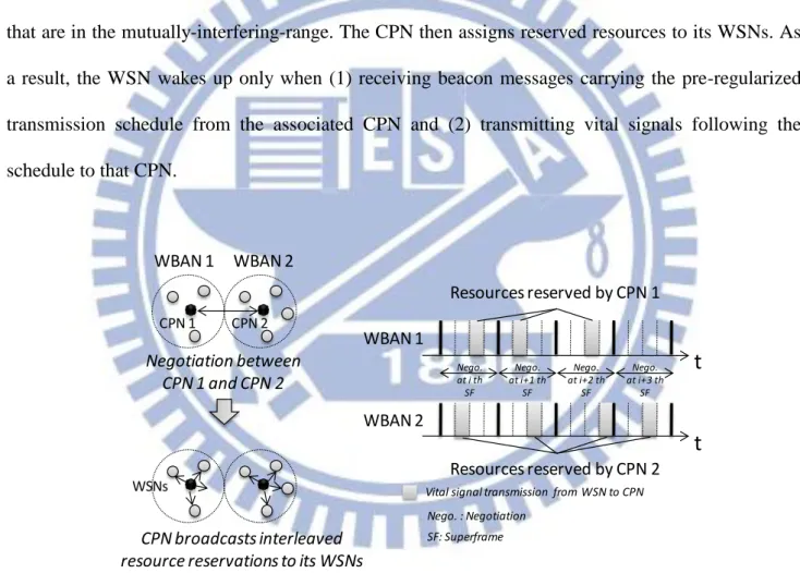
Fig. 3-3, is assumed in this study. The CPN first negotiates the WBAN resources with other CPNs

that are in the mutually-interfering-range. The CPN then assigns reserved resources to its WSNs. As a result, the WSN wakes up only when (1) receiving beacon messages carrying the pre-regularized transmission schedule from the associated CPN and (2) transmitting vital signals following the schedule to that CPN. WBAN 2 WBAN 1 CPN 1 CPN 2 Negotiation between CPN 1 and CPN 2 Resources reserved by CPN 1

t

Resources reserved by CPN 2

t

WBAN 1 WBAN 2

Vital signal transmission from WSN to CPN

Nego. at i th SF

Nego. : Negotiation

CPN broadcasts interleaved resource reservations to its WSNs

WSNs Nego. at i+1 th SF Nego. at i+2 th SF Nego. at i+3 th SF SF: Superframe

Fig. 3-3 CPN-based inter-WBAN scheduling (IWS)

The CPN-based IWS can now be modeled as a unit-disk graph coloring problem. A 2-dimensional randomly constructed graph (in short, random graph) G( , )V E is generated to model the WBAN network. V G( ) represents the set of CPNs; E G( ) represents the set of conflict links between

(37)

25

CPNs. The first step in generating the graph is to randomly deploy nV G( ) vertices in a field to simulate the random positions4 of WBAN users. Consequently, edges are added to connect vertices if the distance between CPNs is equal to or less than the mutually-interfering-range between WBANs (the radius of the unit-disk). In this sense, the graph of CPN-based IWS is similar to that of MANET scheduling. However, they have different resource scheduling strategies. In MANET, each vertex represents a wireless node. MANET focuses on efficient inter-node communication and routing. Hence, “edge” coloring, which models the scheduling of “node-to-node communications”, can be adopted. In contrast, in CPN-based IWS, each vertex represents a sensor group (WBAN). CPN-based IWS tries to resolve the interference between sensor groups belonging to different users. Therefore, “vertex” coloring, which models the scheduling of active “CPN-based sensor groups”, is appropriate. As a result, for CPN-based IWS, a k-coloring of the random graph is labeled V G( )C, where C k, such that adjacent vertices receive distinct colors. The labels are colors, which are mapped to different resource units for associated data transmissions (WSNs to the CPN). Only k resource mappings can be decided when a k-coloring algorithm is excuted once. We assume that every WSN always has data to be transmitted to the CPN. Hence, the coloring is periodically performed to map wireless resources to all these data transmissions. The target of this study is to devise a coloring method that simultaneously satisfies two IWS requirements: (i) low time-complexity and (ii) high spatial reuse.

4 In some cases, waiting lines for example, user positions follow certain rules instead of random deployments, which yield special graphs such as lines or grids. Although these graphs might reflect more real scenarios in our life than the random graph does, they need more complicated analysis skills due to their restrictions of graph formation. Therefore, to make the discussion of the proposed RIC more intuitive, this study focuses on the performance analysis of the random graph.

(38)

26

3.2 Random Incomplete Coloring

The proposed random incomplete coloring (RIC) has two major components: (i) a proposed random-value coloring method and (ii) a proposed incomplete coloring approach. The random value coloring is a low time-complexity coloring method, which is designed for quick IWS. On the other hand, incomplete coloring is a high spatial-reuse coloring approach, which modifies the conventional coloring rule to explore the potential high spatial reuse when k( )G .

3.2.A Random Value Coloring

Random value coloring is a method that realizes oriented coloring. It overcomes two major problems of oriented coloring [28] : fairness and oriented conflict-circle (deadlock circle), as outlined in section 3.1.A. The method of random value coloring is to adopt a random value comparison to generate instant priority differences between all adjacent vertices, as illustrated in Fig. 3-4 (except step 6 for the incomplete coloring).

(39)

27

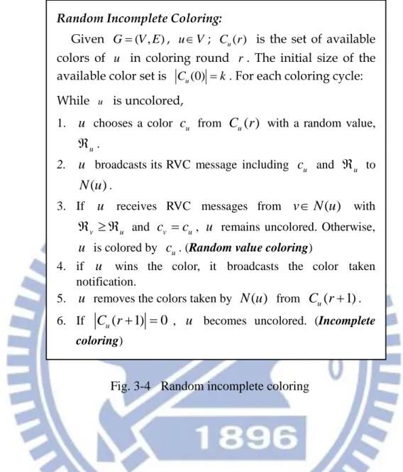
Random Incomplete Coloring:

Given G( , )V E , u V ; C r_u( ) is the set of available colors of u in coloring round r . The initial size of the available color set is C_u(0) k. For each coloring cycle: While u is uncolored,

1. u chooses a color c_u from C r_u( ) with a random value,

u  .

2. u broadcasts its RVC message including c_u and _u to ( )

N u .

3. If u receives RVC messages from vN u( ) with

v u

   and c_v c_u, u remains uncolored. Otherwise, u is colored by c_u. (Random value coloring)

4. if u wins the color, it broadcasts the color taken notification.

5. u removes the colors taken by N u( ) from C r_u( 1). 6. If C r_u( 1) 0 , u becomes uncolored. (Incomplete

coloring)

Fig. 3-4 Random incomplete coloring

In Fig. 3-4, the fairness of random value coloring can be supported if the random values  from different vertices are generated with an identical uniform distribution5. Due to the symmetry between vertices, it is obvious that the probability that a vertex generates the maximum random value (wins the color) among (n1) _{competitors is 1n , where “competitors” means adjacent vertices}

contending for the same color. Thus, each vertex has equal radio resource sharing with its adjacent vertices. Besides, the way that random value coloring avoids an oriented conflict-circle can easily be observed, since it is not possible to have the ordering of the random values of vertices in a circle with

5





( ) 1 ,

(40)

28

a one way orientation     v₁ v₂  vn v₁. The fairness and deadlock-circle-free properties of

the proposed method makes oriented coloring possible to realize for quick IWS.

3.2.B Incomplete Coloring

Incomplete coloring improves spatial reuse by greedily coloring a graph with k( )G . Normally it is not possible to completely color a graph using k( )G colors because color conflict is unavoidable and cannot be resolved6.Thus, incomplete coloring allows uncolored vertices to avoid conflict when vertices run out of k colors, as illustrated at step 6 of Fig. 3-4. Note that when applying incomplete coloring to IWS, the uncolored node means a CPN reserves no resource in that coloring. The WBAN of this CPN becomes temporarily inactive and generates no interference with its neighbor WBANs. The example in Fig. 3-5 demonstrates how incomplete coloring improves spatial reuse (on average).

6

Assume k( )G and G can be completely colored by k colors (adjacent vertices receive distinct colors). However, ( )G is defined as the minimum colors to completely color G and thus

( )

k G contradicts k( )G . As a result, there must be adjacent vertices that receive the same color.

(41)

29 Periodical Complete 3-coloring R G B R R G B 4 1 2 3 4 3 1 2 4 3 Vpc (3a)

Periodical Incomplete 2-coloring

R G R 4 1 2 3 R G R 4 1 2 3 (2a) (2b) R G R 4 1 2 3 G R R 4 1 2 3 (2c) (2d) 3 1 , [2 ] 2 4 Vpc P a  3, [2 ] 1 2 4 Vpc P b  3, [2 ] 1 2 4 Vpc P c  3, [2 ] 1 2 4 Vpc P d  3 [ ] 2 E Vpc 

Resource /Active vertices

Scheduling: t Average Vpc R G B 4 3 1 2 … R G 4 3 2 R G 4 1 2 R G 4 3 1 R G 4 1 3 (2a) (2b) (2c) (2d) … (2a) or (2b) or (2c) or (2d)Could be … … _t

Fig. 3-5 Random incomplete coloring

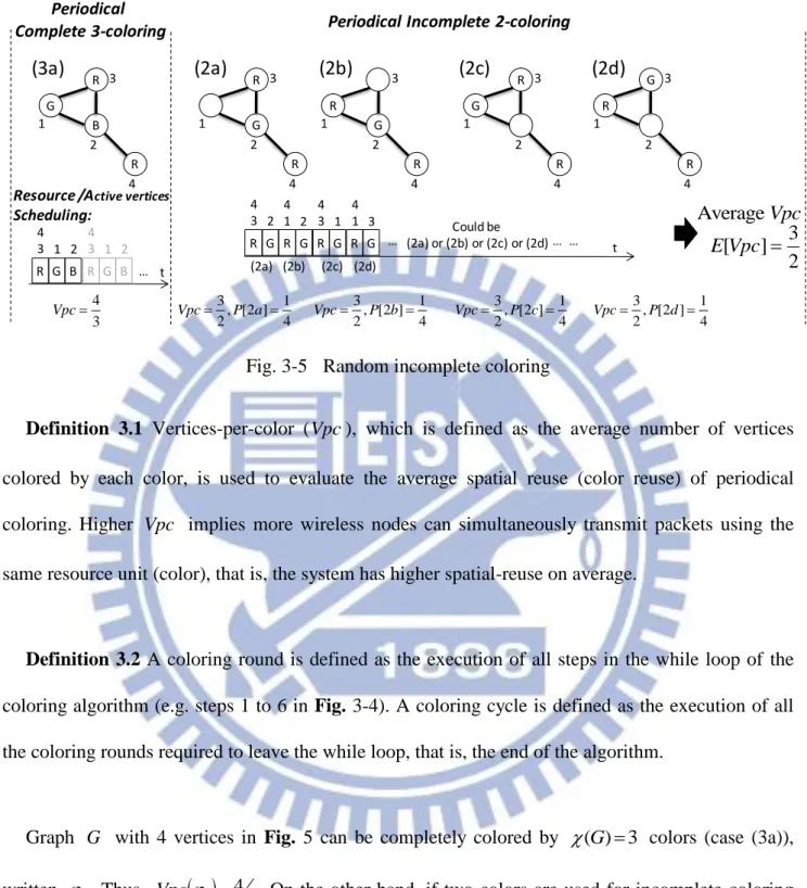
Definition 3.1 Vertices-per-color (Vpc), which is defined as the average number of vertices colored by each color, is used to evaluate the average spatial reuse (color reuse) of periodical coloring. Higher Vpc implies more wireless nodes can simultaneously transmit packets using the same resource unit (color), that is, the system has higher spatial-reuse on average.

Definition 3.2 A coloring round is defined as the execution of all steps in the while loop of the

coloring algorithm (e.g. steps 1 to 6 in Fig. 3-4). A coloring cycle is defined as the execution of all the coloring rounds required to leave the while loop, that is, the end of the algorithm.

Graph G with 4 vertices in Fig. 5 can be completely colored by ( ) 3G  colors (case (3a)), written ₃. Thus,

 

₃ 4

3

Vpc  . On the other hand, if two colors are used for incomplete coloring (k2), written '₂, there are four possible results at the end of the coloring cycle: 2a to 2d. Because 2a to 2d all have 3 vertices colored by 2 colors, 2a to 2d have identical 3

2 Vpc . The probability that each case happens depends on the color contention scheme. Assume a random value

(42)

30

coloring method is adopted. Because cases 2a to 2d are symmetric and vertices 1 to 4 have equal priority in the contention, each case has an identical 1

4 probability of showing up. As a result, when the incomplete coloring with k2, '₂, is iteratively performed,

 

'₂ 3

2 E Vpc_  _

  for

each coloring cycle. There is an increase of 12.5% over

 

₃ 4

3

Vpc  on average.

Of course, the 3-color complete coloring schedules one more resource than the 2-color incomplete coloring in each coloring cycle. In periodical coloring, to schedule the same number of resources, a k-color incomplete coloring (k( )G ) needs ( )G k times more coloring cycles than that of a( )G -color complete coloring, which increases the exchange of coloring messages required for periodical coloring. This could affect the collision probability of coloring messages in a practical IWS implementation. The tradeoffs between spatial reuse and affordable coloring-message exchanges will be closely analyzed in section 3.4.

3.3 Analytical Model of Random Value and Incomplete Coloring

3.3.A

Upper Bound of the time and bit complexity of RIC

With the proposed random value coloring method, the time complexity of RIC can be further decreased from O( log )n [28] to O e W(2ln ) 2n 

 , where W x( ) is the Lambert W function [30]. The

time-complexity (upper bound) of RIC to color a graph with a constant-degree  is calculated. This could be used to observe the time complexity of the 2-D topology model. Because vertices are randomly deployed in the 2-D model, every vertex should have a similar vertex degree. The accuracy of this constant-degree assumption will be verified in the section 3.4.A.

(43)

31

Definition 4.1 Oriented conflict-path (OCP) is defined as a path with all edges having a one-way

orientation and all vertices in this path contending for the same color.

Lemma 4.2 A graph having the longest OCP with l-length (l-vertices) can be colored in at most l rounds.

This lemma is proved by [28], which shows that, in each coloring round, at least one vertex can be colored in the OCP. Thus, a graph with an l-length OCP can be colored within l rounds.

Lemma 4.3 The probability that an OCP has length larger than or equal to i in round rof the

RIC algorithm is less than or equal to

1 1 1 ! r i i k          _{ }         .

For the RIC algorithm, an OCP is only generated when the random values of vertices in the path are in descending order,    _v₁ _v₂ _v₃ (Definition 4.1). Therefore, the probability that an OCP has length larger than or equal to i can be expressed as





1 2 1 1 1 1 1 , [ , ] 1 1 _{(Due to the symmetry of} ₎

1 1 1 1 ! ! i vi v v i i vm vn m i i vm m i i k P k k P Max n m i k k k m k k i k i      _ _           _ _                                                     



 (3-1)

Where k is the number of colors used in the RIC. The length of the OCP can only decrease or stay the same during the coloring. Hence, to make sure the length of an OCP is larger than or equal to

(44)

32

i in round r, the length of this OCP should always be larger than or equal to i from round 1 to round r. Therefore, the probability that an OCP has length larger than or equal to i in round r is

less than or equal to

1 1 1 ! r i i k          _{ }         .

Theorem 4.4 Given a graph with n vertices and constant degree , the time complexity of the RIC algorithm for any number of colors is O e_ W(2ln ) 2n _ rounds, where W x( ) is the Lambert W function.

Proof: A two-phase analysis, which is similar to [28, 31], is adopted to calculate the time

complexity of the proposed RIC algorithm. Phase I lasts from the first coloring round to _r th

 ,

(2ln ) 2 10 W n

r_ e rounds; Phase II lasts from



r_1



th rounds to the end of the coloring cycle. A graph may contain multiple OCPs during the coloring. At the end of Phase I, we prove that the length of any OCP of the graph will be confined by the length l_eW(2ln ) 2n with a high probability. According to lemma 4.2, this graph can be further colored with at most eW(2ln ) 2n coloring rounds in Phase II. Thus, the total coloring rounds can be proved to be

(2ln ) 2 (2ln ) 2 (2ln ) 2

10 W n W n W n

O_ e _O e_ _O e_ _.

At the end of Phase I, the length of any OCP will be proven to be confined by the length

(2ln ) 2

W n

l_e with a high probability. This can be a dual proof: there is a low probability that at least one OCP of the graph is of length larger than l_ at the end of Phase I. This probability is denoted as

[ ]

P . The probability of an OCP in such event is denoted as P l r_

 

_ l__

(45)

33

length of the OCP in round r_. Also, in a graph with n vertices, _ni_{is the maximum}7_{number of}

OCPs with length i. Therefore,

 

1 1 1 1 [ ] 1 1 (Lemma 4.3) ! n _i i l n _i i l r i n _i i l P n P l r i n P l r i n i k                                  _{ }                   



 (3-2)

For simplicity in the following calculation, the approximation of the factorial term, !

i i i e e          , is applied. Thus 1 1 1 1 1 1 1 1 ! r r i i n _i n _i i i l n _k _i i l n _k i e _e             _{ }  _{ }  _{ }  __{ } _ _{ }  __{ } _         _ _ _ _    _ _          



. Each term in the summation

can be simplified to ₁₀10 10₁₀ 1 ₁₀ l i l i i l k e n e k i                  _ _        

  , which is less than or equal to ₇

i l n i       due to (1) (1) (1) i l i l i l iO  O O  _{(recall that i l}   ). Also, 2 7 7 i l l n n i l             _ _  and _l _eW(2ln ) 2n  lead to 2 l n l  

 (recall that zW z( ) exp[W z( )] , for any complex number

z

). Therefore,

7 5 1 1 [ ] n i l n P n n    





 , which approaches 0 as n. As a result, at the end of Phase I, the lengths

of any OCPs confined by l_ eW(2ln ) 2n are proved with a high probability. The upper bound of total rounds that the RIC algorithm requires is the summation of the maximum rounds of Phases I and II,



₁₀ W(2ln ) 2n

 

W(2ln ) 2n

 

W(2ln ) 2n



O e O e O e , Q.E.D.

7

Because each OCP could start from any of l eW(2ln ) 2n vertices. Also, each vertex has  adjacent vertices in the constant  degree graph, so there are i_{possible combinations to generate an OCP with}

多人無線近身網路系統

國 立 交 通 大 學

電子工程學系電子研究所

博 士 論 文

多人無線近身網路系統

Multiuser Wireless Body Area Networks

研 究 生 ：程士恒

指導教授 ：黃經堯 博士

國 立 交 通 大 學

電子工程學系電子研究所

博 士 論 文

多人無線近身網路系統

Multiuser Wireless Body Area Networks

研 究 生 ：程士恒

指導教授 ：黃經堯 博士

多人無線近身網路系統

Multiuser Wireless Body Area Networks

研 究 生 ：程士恒 Student: ShihHeng Cheng

指導教授 ：黃經堯 博士 Advisor: ChingYao Huang

國立交通大學

電子工程學系 電子研究所

博士論文

A Dissertation

Submitted to Department of Electronics Engineering and

Institute of Electronics

College of Electrical and Computer Engineering

National Chiao Tung University

in partial Fulfillment of the Requirements

for the Degree of

Doctor of Philosophy

in

Electronics Engineering

Aug 2012

Hsinchu, Taiwan, Republic of China

多人無線近身網路系統

研 究 生 ：程士恒 指導教授 ：黃經堯 博士

國 立 交 通 大 學

電 子 工 程 學 系 電 子 研 究 所

摘要

Multiuser Wireless Body Area Networks

Student: ShihHeng Cheng Advisor: Dr. ChingYao Huang

Department of Electronics Engineering

and

Institute of Electronics

National Chiao Tung University

Abstract

Acknowledgements

Contents

List of Tables

List of Figures

Chapter 1

Introduction of Multiuser WBANs

1.1 Network Architecture

1.2 Design Challenges of Multi-User WBAN MAC

Chapter 2

Analysis of multiuser interference

(a)

CPN

WSN

ECG

(b)

2.1 WBAN Performance Model of Beacon and Slotted CSMA/CA

Modes

J

J

J

J

P

P



















2.2 Analysis and Hybrid Mode

2.2.A

國立交通大學

博士論文

研究生：程士恒

指導教授：黃經堯博士

國立交通大學

博士論文

研究生：程士恒

指導教授：黃經堯博士

研究生：程士恒 Student: ShihHeng Cheng

指導教授：黃經堯博士 Advisor: ChingYao Huang

電子工程學系電子研究所

研究生：程士恒指導教授：黃經堯博士

國立交通大學

電子工程學系電子研究所