Do the Chinese Bourses (Stock Markets) Predict Economic Growth?

全文

(1)International Journal of Business and Economics, 2009, Vol. 8, No. 3, 201-211. Do the Chinese Bourses (Stock Markets) Predict Economic Growth? Jeffrey E. Jarrett* Faculty of Management Science and Finance, University of Rhode Island, U.S.A. Xia Pan Lingnan College, Sun Yat-sen University, Guangzhou, China Shaw Chen Faculty of Management Science and Finance, University of Rhode Island, U.S.A.. Abstract We study the relationship between the Chinese macroeconomy and the Chinese stock markets, i.e., the bourses in Shanghai and Shenzhen. With this goal, we utilize multiple Granger causality and Geweke linear dependence and examine likelihood ratio statistics between two sectors of the Chinese economy: the Chinese economic prosperity score (EPS)—and its departure from a “healthy level” (EPS-D)—and composite indexes for Chinese securities markets—Shanghai composite (SH) and Shenzhen composite (SZ). The data cover nine years. The authors found no evidence that SH and SZ Granger cause economic prosperity. The evidence supports the notions that Chinese stock markets respond greater to changes in EPS-D than to EPS and that the SZ is more sensitive to changes in the economy than the SH. Key words: Granger causality; Geweke linear dependence; likelihood ratio tests; vector autoregression JEL classification: G15; G17; F21. 1. Purpose Investment opportunities in Chinese financial markets (Chen, 1991; Cheung and Ng, 1998; Liaw, 2007) describe China as an economic power offering tremendous business and economic opportunities. However, its financial markets are still not fully developed when analyzed by methods developed by financial economists (Fama, 1990, 1991; Wei and Wong, 1992; Zhong et al., 1999, hereafter ZGL). In contrast with their Western counterparts (and Japan), Chinese financial markets are highly speculative. The majority of participants are individuals and Received June 3, 2009, revised December 1, 2009, accepted December 15, 2009. * Correspondence to: Faculty of Management Science and Finance, University of Rhode Island, 7 Lippitt Road/Ballentine Hall, Kingston, RI 02881-0802, U.S.A. E-mail: jejarrett@mail.uri.edu..

(2) 202. International Journal of Business and Economics. naïve investors who lack the knowledge of investing and a large enough fund base for sophisticated investing in developed financial markets. Moreover, government interventions are far more frequent and stronger than those in developed nations. Thus, the relationship between stock markets and real economic activity remains a compelling topic for empirical investigation. Thomas (2001) discusses in detail the workings of the Shanghai bourse over its illustrious history, offering insights into the characteristics of the financial market, including the behavior of both domestic and foreign investors in this market. It is a descriptive history including aspects in the twentieth but not twenty-first century. Another interesting report on these same markets is by Gao (2002), who notes both the strengths and shortcomings of Chinese markets. He used phrases such as “unusual market structure,” “market manipulation and speculation,” and “dominated by a limited number of large cap stocks,” “multitude of small cap stocks,” “widespread government holdings,” and the like in characterizing these markets. Furthermore, he argues for greater regulatory control in markets to foster an environment in which the stock markets can survive. These studies indicate important differences between Western-oriented stock markets and Chinese bourses. Hence the culture and the way in which Chinese markets do business should not be judged by the standards used to judge markets in the US, Japan, and markets in Central and Western Europe. Other researchers (Eun and Huang, 2007; Ng and Wu, 2007; Su 1998; Wang et al., 2004) investigated the rapid growth in Chinese stock markets and why they became increasingly important for investors in international markets. The markets play a vital role in privatizing China’s state-owned enterprises and spreading ownership among domestic and international investors. With energetic growth in China and commitment of the authoritarian government to privatization, we expect that the Chinese stock markets will continue to grow. Whether the stock markets are a useful barometer of the growth and conditions of the economy is the subject of an ongoing debate. ZGL analyzed this question by investigating whether the Shenzhen and Shanghai stock markets have separate cointegration with the Chinese economic prosperity score (EPS) and departure from the “healthy level” of this score (EPS-D). By Granger (1969) causality (see Toda and Phillips, 1994; Dufour et al., 2006) they analyzed pairs of variables separately, the Granger causalities between the Shanghai stock index and EPS and between the Shanghai stock index and EPS-D. They concluded that the Chinese economic prosperity is the Granger cause of the growth in the stock market. The same could not be concluded about the relationship between economic growth and the Shenzhen stock market. They presented the test results of Granger causality but avoided concluding whether the stock markets influence the economy. In this study we will present additional evidence concerning the relationship between the Chinese macroeconomy and the bourses in Shanghai and Shenzhen. ZGL further found indications that the Shanghai and Shenzhen bourses do not have separate cointegration with the Chinese EPS and EPS-D. Variations of stock.

(3) Jeffrey E. Jarrett, Xia Pan, and Shaw Chen. 203. market indexes do cointegrate with the variation of EPS and the change of EPS-D. In addition, they found evidence of Granger causalities between the Shanghai stock index and EPS and EPS-D and between the Shenzhen stock index and EPS and EPSD. Their conclusion was that economic growth Granger causes rises in the bourses. One exception was the relationship between the economy and rises in the Shenzhen stock index. They avoided concluding that the stock markets Granger cause rises in the size of the economy. In the present study, we employ multi-group vector autoregression (VAR) to ascertain Granger causality between the two bourses and the Chinese macroeconomy. Specifically, we treat the Shanghai and Shenzhen bourses as one group and the EPS and EPS-D as a second group. Thus, we can go much further in establishing the linkages between growth in the macroeconomy and the two financial markets and in turn shed greater light on the roles that each economic entity plays. By following and improving upon the methods of ZGL for a later time period, we will verify whether or not their research conclusions hold under a newer and more thorough investigation. Multi-group VAR is superior to pairwise VAR because pairwise applications may result in conflicting causality analysis. For example, the macroeconomic group (Group A) may have several variables and the financial market group (Group B) may also contain a number of variables. A variable in group A, say A1, may lead to variation in a member of group B, say B1, however, the conclusion that A1 leads B1 is often invalid. Furthermore, concluding that B1 leads A1 may also be invalid. Using multi-group VAR, we can explain whether or not group A leads group B. We can also identify whether or not group B leads group A. If pairwise interaction occurs, we can allow each group to contain only one grouped VAR and we can assess the individual relationships. A pairwise VAR model is a special case of the multi-group VAR model. Similarly, while pairs of variables can be estimated only by providing measures of each pair of variables, Geweke (1984) linear dependence provides a general measure of the association between the two groups. 2. Multiple Granger Causality and Geweke Linear Dependence Granger causality tests (1969) are a useful method for drawing clear conclusions in a simple two-dimensional system, but they should be used with great care. The test may be performed using two vectors and is therefore not a twodimensional system in the usual sense. Another potentially serious problem is the choice of the sampling period; for example, a long sampling period may hide the causality. In addition, VAR (Chan, 2002, pp. 124-135) systems for monthly data may yield serious measurement errors due to seasonal adjustment procedures. Geweke et al. (1983) and Geweke (1984) propose measures of linear dependence and feedback for multiple time series that are stationary (at least in the broad statistical sense that there is no upward or downward trend in the average over time, no change in the variability about the average over time, and no seasonal pattern in the data—see O’Donovan, 1983, p. 24), autoregressive, and purely.

(4) 204. International Journal of Business and Economics. nondeterministic. The measure of linear dependence is the total of the linear feedback from the first series to the second, the linear feedback from the second to the first, and the instantaneous linear feedback. When feedback (or causality) is absent, the measure will be zero (it is never negative). Furthermore, the measure of linear feedback from one series to another can be additively decomposed. Hence, using this notion of linear feedback with that of Granger causality, we can attempt to analyze how the macroeconomy of China and the variation in the Chinese stock market are related. Hence, these methods coupled together can give us a more meaningful result than simply finding the correlation between the macroeconomy and the variation in the stock markets. Previous studies of stock market analysis utilized these methods successfully. Geweke (1984) studied linear dependence and spectral feedback for grouped multivariate time series. Pan (2007) applied linear dependence and spectral feedback to examine the relationship between grouped economic variables and stock market indexes. Placing economic variables into one group and stock market variables into another, he estimated the between-group relationship within the US, within Japan, and within the European Union. The feedback spectra for grouped variables were calculated and reported. There is a risk, however, that he determined feedback spectra on variables that were possibly nonstationary in level and that he found the patterns of the feedback spectra providing information about the cyclical effect between the variable groups. Simple Granger causality is between two variables. The VAR between these variables, y1 and y 2 , is as follows: y1t = c1 + A1 ( L) y1t + A2 ( L) y2 t + e1t , y 2t = c2 + B1 ( L) y1t + B2 ( L) y 2t + e2t ,. where A1 ( L) , A2 ( L) , B1 ( L) , and B2 ( L) are arrays of a lag operator with order p , for example A1 ( L) = a11 L + a12 L2 + L + a1n Lp . If the scalar coefficients in A2 ( L) are all zeros, y 2 does not Granger cause y1 . Stated differently, the values of y 2 in the previous time periods do not influence the current value of y1 . Similarly, if B1 ( L) is zero, y1 does not Granger cause y 2 . ZGL tested the separate hypotheses of A2 ( L) and B1 ( L) equaling zero for each pair of the variables. Multiple Granger causality is the result of VAR between two groups of r r variables and not two variables alone. Let y1t and y2 t denote vectors of lengths n1 and n2 consisting of several variables deemed as a group of variables jointly r r describing one feature of reality. Similarly, let x1t and x2 t denote vectors of r r lengths n1 p and n2 p consisting of all the lagged vectors of y1t and y2 t ; that is, rt rt rt rt rt rt rt rt x1t = ( y1, t −1 , y1, t −2 , K, y1, t − p ) and x2 t = ( y2 , t −1 , y2 , t −2 , K , y2 , t − p ) . The VAR is written: r r r r r y1t = c1 + A1 x1t + A2 x2 t + e1t , r r r r r y 2t = c2 + B1 x1t + B2 x2 t + e2 t ,.

(5) Jeffrey E. Jarrett, Xia Pan, and Shaw Chen. 205. where the constant items and the error terms are all vectors for the respective variable groups, and the A1 , A2 , B1 , and B2 are matrices of coefficients without r lag operators. Analogous to the pairwise VAR, if A2 is a zero matrix, y 2 t does r r not jointly Granger cause y1t . If B1 is a zero matrix, y1t does not jointly Granger r cause y 2 t . With this multi-group VAR, we determine the linear feedback (Granger causality) between two groups of variables as a whole instead of between two variables individually. The benefit of multi-group VAR is the one feature describes several variables. We may now observe, for example, that one variable in group 1 Granger causes a variable in group 2 but that a second variable in group 1 does not Granger cause the same variable in group 2. By this reasoning, whether the feature described in group 1 is the Granger cause of the feature described in group 2 may not be conclusive. Multi-group VAR avoids this inconclusive result because it jointly includes all the effects of all the variables in all variables in all the periods of interest and the significance of the whole joint effect is determined statistically. An example of this analysis is given in Lemmens et al. (2008), who decomposed Granger causality over a spectrum, allowing them to disentangle potentially different Granger causality relationships over different frequencies. This yielded new and complementary insights compared to traditional versions of Granger causality. The usefulness of Granger results are discussed in detail and shown to support the use of the Granger causality analysis utilized in this and other studies. Geweke et al. (1983, 1984) measured linear dependence on the basis of likelihood ratio analysis. Our research hypothesis is that there is no association between the two groups of variables. We test this hypothesis using a likelihood ratio test (LRT); see for instance Felsenstein (1981), Huelsenbeck and Crandall (1997), Huelsenbeck and Rannala (1997), and Swofford et al. (1996). While the focus of this study is using the LRT to compare two competing models, under some circumstances one can compare two competing trees estimated using the same likelihood model. There are many additional considerations; see for example Kishino and Hasegawa (1989), Shimodaira and Hasegawa (1999), and Swofford et al. (1996). Barnett et al. (1989) present fundamental new research on the analysis of complicated outcomes in relatively simple macroeconomic models. In essence, the LRT determines (1) the Granger causality between group 1 and group 2, (2) the Granger causality between group 2 and group 1, and (3) the instantaneous feedback (no time lags) between the two groups. Geweke (1984) linear dependence combines the three feedbacks to measure the scale of linear dependence between the two groups of variables as a whole. The value of this approach is that the evidence given by the Geweke linear dependence measure provides reliable measures of the joint relationships between the groups of variables examined in this study..

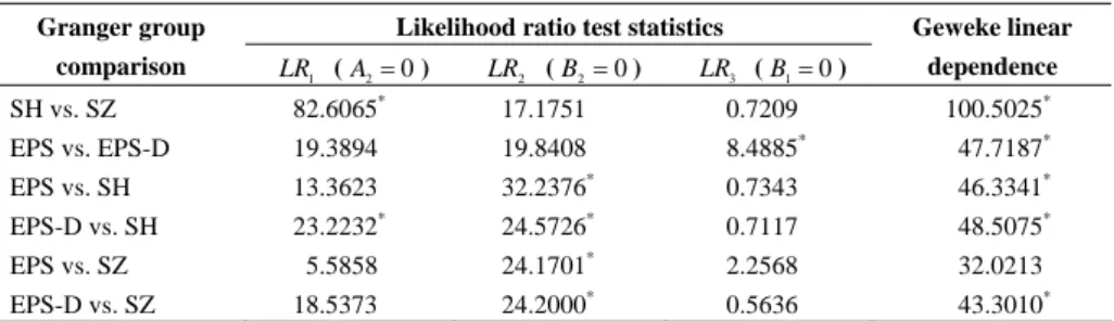
(6) 206. International Journal of Business and Economics. 3. Data Selected for Study. Following the study of ZGL for the Chinese bourses in Shanghai and Shenzhen, we selected the composite index for each market. We identified the longest time period that would lead to interpretable results, resulting approximately nine years of data. Short periods (e.g., two or three or even four years) are usually too brief to overcome the effects of short-term disturbances in economic data and do not provide adequate statistical power to identify significant events and factors. We could have examined alternative measures of Chinese stock market behavior; there are studies using such indicators as the Dow Jones China 88. However, the purpose of these other studies (Fama and Schwert, 1977; Fama, 1990, 1991; Chen, 1991; Wei and Wong, 1992; Cheung and Ng, 1998) differed greatly from the purpose of this study. Furthermore, we gathered our data from private sources which better reflected existing Chinese financial markets. The index represents monthly closing composite returns over the early nine year time period for the financial markets. New indexes are now being prepared, and when they have a sufficiently long history one will be able to study them as well. The titles given to the indexes utilized in this study differ in Chinese but they measure the composite change in the prices and returns for securities listed on each of the two bourses. To measure the size of the total Chinese economy, we utilized the Chinese Economic Prosperity Score (EPS). This score is produced by a department of the National Statistics Bureau of China. It combines most data collected about the entire Chinese economy. Further, this score indicates the scale of the prosperity in the economy, with a score of 30 deemed to represent a healthy economic level. In turn, a departure from the healthy level measures the degree to which the economy differs from a healthy or level in either direction. This departure is the absolute value of the difference and indicates the degree to which the economy is expanding or contracting relative to the base line. Hence, we also include this measure (denoted EPS-D) as one of the macroeconomic variables. The Shanghai composite (SH) and Shenzhen composite (SZ) are the variables indicating the Chinese stock markets and together comprise the first group in our multi-group VAR. The second group, representing the Chinese economy, contains EPS and EPS-D. Data collected for this study are for a nine year period ending with the latest data available for inclusion in this study. 4. Data Analysis and Results. Table 1 contains the results of the LRT statistics for the VAR and the Geweke linear dependence measures between the Chinese bourses and the Chinese economy. We report LRT statistics for p = 12 month lags, and our methodology is similar to that of ZGL. The LRT statistics LR1 , LR2 , and LR3 test the hypothesis that group 2 does not Granger cause group 1, that group 1 does not Granger cause group 2, and that there is no instant feedback between groups 1 and 2 (i.e., the influence between.

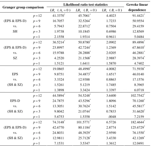
(7) Jeffrey E. Jarrett, Xia Pan, and Shaw Chen. 207. the two groups is limited to within a month). The Geweke linear dependence measure is the sum of LR1 , LR2 , and LR3 . Statistical significance is based on comparing test statistics with chi-squared distributions. Table 1. VAR and Geweke Linear Dependence between the Chinese Economy and the Chinese Bourses Likelihood ratio test statistics. Granger group comparison SH vs. SZ EPS vs. EPS-D. LR1 ( A2 = 0 ) 82.6065* 19.3894. LR2 ( B2 = 0 ) 17.1751. Geweke linear. LR3 ( B1 = 0 ). 19.8408. 8.4885. dependence 100.5025*. 0.7209 *. 47.7187*. 32.2376. *. 0.7343. 46.3341*. 24.5726. *. 0.7117. 48.5075*. 24.1701. *. 2.2568. 32.0213. EPS-D vs. SZ 18.5373 24.2000* * Notes: denotes significance at the 5% level.. 0.5636. 43.3010*. EPS vs. SH EPS-D vs. SH EPS vs. SZ. 13.3623 23.2232. *. 5.5858. We see in Table 1 that the Shenzhen bourse leads the Shanghai bourse and the linear dependence between the two bourses is strong. There is no evidence that either the prosperity score or its departure from a healthy level lead the other. The instant feedback is very strong, with statistically significant linear dependence. We conclude that the Shanghai and Shenzhen bourses do not Granger cause economic prosperity. The Shanghai bourse Granger causes departures of the economy from a healthy level, but this conclusion does not hold for the Shenzhen bourse. In each case, the economy as represented in this study Granger causes changes (expansions and contractions) in the values of the bourses. The dependence between the Shenzhen bourse and economic prosperity is not strong. Furthermore, we confirm the phenomenon that changes in the economy lead the stock markets and not the other way around. We present in Table 2 the results of the multi-group VAR. We find that Chinese markets Granger cause the economy when we consider a lag up to 12 months. If the lag is 9 months or less, there is no evidence of Granger causality. In contrast, the economy leads the bourses when lags exceed 1 month. We believe that lead time effects can better be studied in the future by spectral analysis and point estimation of frequencies; however, our findings suggest that this effect occurs. We thus obtain a rough idea about the length of causality. Broadly, the bourses are not leading indicators of changes in the Chinese economy. We find that the linear dependence between the Shanghai bourse and the Chinese economy is not strong. The Geweke linear dependence measures do not reject the hypothesis that there were no relationships between the variation in the returns to Shanghai bourse and Chinese economy as measured in this study when the lag was 9 months or less. This result differs from ZGL. Since they did not employ Geweke linear dependence, their conclusion was based on a simpler analysis. In addition, we should note that the feedback hypothesis for the Shenzhen bourse implies a more immediate impact than on the Shanghai bourse. Stated differently,.

(8) 208. International Journal of Business and Economics. the Chinese macroeconomy impacts the Shenzhen bourse more quickly than it impacts the Shanghai bourse. Although neither is a very good barometer of the Chinese economy, the effects of the economy on these bourses differ. Table 2. VAR and Geweke Linear Dependence between the Chinese Economy and the Chinese Bourses Granger group comparison. p = 12. Likelihood ratio test statistics. LR1 ( A2 = 0 ) 41.3370*. LR2 ( B2 = 0 ). LR3 ( B1 = 0 ). Geweke linear dependence. 45.7061*. 4.4023. 91.4421*. *. (EPS & EPS-D). p=9. 16.7057. 32.5264. 1.7233. 50.9554. vs.. p=6. 5.7943. 22.8712*. 0.7504. 29.4159. SH. p=3 p =1. 1.9738 2.1558. 10.1845 1.9314. 0.6986 0.9611. 12.8569 5.0484. p = 12. 36.5214*. 50.8780*. 2.0902. 89.4896*. *. (EPS & EPS-D) vs. SZ. p=9 p=6 p=3. 23.8997 15.9788. 42.7244 28.2888*. 1.2369. 67.8610*. 2.0205. 46.2881*. 4.2520. *. 28.3974* 4.7402. 21.1568. p =1. 1.5121. 1.6411. 2.9887 1.5870. p = 12. 19.0865. 48.4990*. 4.0082. 71.5938*. *. 1.6517 0.8863. 46.0140 17.1576 8.3965 6.0718. EPS vs.. p=9 p=6. 9.8751 3.3324. 34.4873 12.9388. (SH & SZ). p=3 p =1. 1.5261 1.3898. 5.1219 3.3424. 1.7485 1.3397. p = 12. 44.5894*. 54.5248*. 3.6400. 102.7542*. *. EPS-D vs. (SH & SZ). p=9 p=6 p=3. 24.7875 13.3051. 43.5296 30.7624*. 1.8096. 70.1260*. 1.5142. 45.5817*. 9.8042. *. 0.7833 .0048. 31.6620* 7.2159. 101.5771*. 6.5726. 182.4644*. *. p =1. 5.6753. p = 12. 74.3148*. p=9 p=6. 21.0744. 1.5358. 42.6770 24.8031. 80.1184 48.3929*. 2.8774. 125.6729*. 2.9590. 76.1550*. 12.9811. 25.7128. *. p =1 7.1531 Notes: * denotes significance at the 5% level.. 3.5347. 3.4330 1.3612. 42.1269* 12.0491. (EPS & EPS-D) vs. (SH & SZ). p=3. If we further examine the relationships between the individual macroeconomic indicators, we find a stronger relationship between the variation in the bourses and the departure from the healthy economy than the relationship between the variation in the bourses and the prosperity score alone. This indicates that the EPS-D contains more information concerning changes in stock market activity than the prosperity score alone. Hence, EPS-D is a better barometer of future stock market fluctuations than the EPS indicator..

(9) Jeffrey E. Jarrett, Xia Pan, and Shaw Chen. 209. 5. Summary and Conclusions. We surmise that variation in the market indicators of the returns to investors are not reliable predictors of changes in the broad Chinese economy. As Liang and Teng (2001) found unidirectional causality from economic growth to financial development, we found no evidence that the opposite direction occurred. The returns to the investments in the Chinese bourses respond greater to the sensitivity of absolute changes in the economy than to the economy itself taken in its entirety. In addition, the Shenzhen bourse is more sensitive to changes in the economy than the Shanghai bourse. The Shenzhen bourse contains many more small capitalization stocks than the Shanghai bourse which may be the reason this exchange is more sensitive to changes in the general economy. Large firms, which are more characteristic of the Shanghai exchange, may drive this market to be less sensitive because larger firms are more resilient. The differing characteristics of the Chinese bourses could be related to the lack of maturity in the Chinese security markets and the rapid transformation of the Chinese economy. If we compare the size of these security markets in China to the size of the economy, we find that the security markets are a much smaller part of the economy than in other nations. Basically, these security markets are a relatively small portion of the economy and thus have little influence on the Chinese national economy. This result is not inconsistent with studies of the errors in forecasting returns for listed Chinese firms. Su and Fleisher (1999) studied the difficulties in forecasting returns for Chinese firms, supporting the notion that Chinese stock returns and prices are not very good barometers of the changes in the Chinese macroeconomy. Further, we should note as the securities markets grow, there still will be great need to police the securities markets to ensure that these markets operate both efficiently and without corruption such as insider trading. As these markets increase in size, one expects that these markets will contain features and institutions more closely associated with the large Western and Japanese markets. References. Barnett, W. A., J. Geweke, and K. Shell, (1989), Economic Complexity: Chaos, Sunspots, Bubbles, and Nonlinearity: Proceedings of the Fourth International Symposium in Economic Theory and Econometrics, England: Cambridge University Press. Chan, N. H., (2002), Time Series: Applications to Finance, New York, NY: Wiley. Cheung, Y-W. and L. Ng, (1998), “International Evidence on the Stock Market and Aggregate Economic Activity,” Journal of Empirical Finance, 5, 281-296. Dufour, J-M., D. Pelletier, and E. Renault, (2006), “Short Run and Long Run Causality in Time Series: Inference,” Journal of Econometrics, 132(2), 337-362. Eun, C. S. and W. Huang, (2007), “Asset Pricing in China’s Domestic Stock Markets: Is There a Logic?” Pacific-Basin Finance Journal, 15(5), 452-480..

(10) 210. International Journal of Business and Economics. Fama, E., (1990), “Stock Returns, Expected Returns, and Real Activity,” Journal of Finance, 45, 1089-1108. Fama, E., (1991), “Efficient Capital Markets: II,” Journal of Finance, 46, 1575-1617. Fama, E. and G. Schwert, (1977), “Asset Returns and Inflation,” Journal of Financial Economics, 5, 115-146. Felsenstein, J., (1981), “Evolutionary Trees from DNA Sequences: A Maximum Likelihood Approach,” Journal of Molecular Evolution, 17(6), 368-376. Huelsenbeck, J. P. and K. A. Crandall, (1997), “Phylogeny Estimation and Hypothesis Testing Using Maximum Likelihood,” Annual Review of Ecology and Systematics, 28, 437-466. Huelsenbeck, J. P. and B. Rannala, (1997), “Phylogenetic Methods Come of Age: Testing Hypotheses in an Evolutionary Context,” Science, 276, 227-232. Gao, S., (2002), “China Stock Market in a Global Perspective,” Dow Jones Indexes, September, 1-48. Geweke, J., R. Meese, and W. Dent, (1983), “Comparing Alternative Tests of Causality in Temporal Systems: Analytic Results and Experimental Evidence,” Journal of Econometrics, 21, 161-194. Geweke, J., (1984), “Inference and Causality in Econometric Time Series Models,” in Handbook of Econometrics, Vol. 2, Z. Griliches and M. Intrilligator eds., Amsterdam: North Holland. Granger, C. W. J., (1969), “Investigating Causal Relations by Econometric Models and Cross-Spectral Methods,” Econometrica, 37(3), 424-438. Kishino, H. and M. Hasegawa, (1990), “Converting Distance to Time: Application to Human Evolution,” Methods Enzymol, 183, 550-570. Lemmens, A., C. Croux, and M. G. Dekimpe, (2008), “Measuring and Testing Granger Causality over the Spectrum: An Application to European Production Expectation Surveys,” International Journal of Forecasting, 24(3), 414-431. Liang, Q. and J. Z. Teng, (2006), “Financial Development and Economic Growth: Evidence from China,” China Economic Review, 17(4), 395-411. Ng, L. and F. Wu, (2007), “The Trading Behavior of Institutions and Individuals in Chinese Equity Markets,” Journal of Banking and Finance, 31(9), 2695-2710. O’Donovan, T. M., (1983), Short Term Forecasting: Introduction to the Box-Jenkins Approach, Chichester: John Wiley, 24. Pan, X., (2007), “The Linear Dependence and Feedback Spectra between Stock Market and Economy,” International Journal of Theoretical and Applied Finance, 10(3), 437-447. Shimodaira, H. and M. Hasegawa, (1999), “Multiple Comparisons of LogLikelihoods with Applications to Phylogenetic Inference,” Molecular Biology and Evolution, 16, 1114-1116. Swofford, D. L., G. J. Olsen, P. J. Waddell, and D. M. Hillis, (1996), “Phylogenetic Inference,” in Molecular Systematic, 2nd edition, D. M. Hillis, C. Moritz and B. K. Mabel eds., Sunderland, MA: Sinauer Associates, 407-543..

(11) Jeffrey E. Jarrett, Xia Pan, and Shaw Chen. 211. Su, D., (1998), “The Behavior of Chinese Stock Markets,” in Emerging Capital Markets, J. J. Choi and J. A. Doukas eds., Westport Ct.: Quorum Books, 253273. Su, D. and B. M. Fleisher, (1999), “Why Does Return Volatility Differ in Chinese Stock Markets?” Pacific-Basin Finance Journal, 7, 557-586. Thomas, W. A., (2001), Western Capitalism in China: A History of the Shanghai Stock Exchange, Aldershot: Ashgate. Toda, H. Y. and P. C. B. Phillips, (1994), “Vector Autoregression and Causality: A Theoretical Overview and Simulation Study,” Econometric Reviews, 13, 259285. Wang, J., B. M. Burton, and D. M. Power, (2004), “Analysis of the Overreaction Effect in the Chinese Stock Market,” Applied Economic Letters, 11(7), 437-442. Wei, K. and K. Wong, (1992), “Tests of Inflation and Industry Portfolio Stock Returns,” Journal of Economics and Business, 44(1), 77-94. Zhong, R. S., L. Gu, and C. B. Lui, (1999), The Empirical Statistical Analysis of Chinese Stock Markets, Beijing: China Financial and Political Economics Press..

(12)