隨機數位樹上加法性參數之機率分析

(1)

國立交通大學

應用數學系

博士論文

隨機數位樹上加法性參數之機率分析

Probabilistic Analysis of Additive Shape

Parameters in Random Digital Trees

研究生:

李忠逵

(2)

(3)

隨機數位樹上加法性參數之機率分析

Probabilistic Analysis of Additive Shape

Parameters in Random Digital Trees

研究生：李忠逵

Student: Chung-Kuei Lee

指導教授：符麥克

Advisor: Michael Fuchs

國立交通大學

應用數學系

博士論文

A Thesis

Submitted to Department of Applied Mathematics College of Science

National Chiao Tung University in partial Fulfillment of the Requirements

for the Degree of Doctor of Philosophy

in

Applied Mathematics

June 2014

(4)

(5)

隨機數位樹上加法性參數之機率分析

研究生: 李忠逵指導教授: 符麥克

國立交通大學

應用數學系

摘要

自圖靈獎得主高納德 (D. E. Knuth) 於 1963 年首開先河後，演算法分析成為了一個在數學和理論計算機科學中皆具相當重要性的研究領域。本領域的主要目標之一在於取得對演算法之隨機行為的全面了解。除此之外，資料結構的漸進性質也是演算法分析所關注的重要議題。數位樹家族是在計算機和資訊科學中最常被使用的資料結構之一。在本論文中，我們藉由研究數位樹的加法性構型參數探討了此一資料結構的眾多漸進性質。本論文的第一部份是對數位樹家族進行一個完整的介紹。內容包括了構造方式、我們將使用的隨機模型、已知的研究成果和相關的數學工具。我們也將利用一些例子來解釋這些數學工具在過去的研究中是如何被使用的。第二部分則是我們新獲得的研究成果，包括了 Poisson-Laplace-Mellin 方法的新應用以及一套可用來證明隨機數位樹加法性構型參數的中央極限定理的理論框架。過去使用 Poisson-Laplace-Mellin 方法所獲得的結果大多數是有關線性成長的構型參數的，我們在本論文中運用 Poisson-Laplace-Mellin 方法對許多非線性成長的構型參數進行了研究並且推導出了這些參數的期望值和變異數的漸進表示。我們還建立了一套可以近乎” 自動” 證明構型參數的中央極限定理的理論框架_{− 只要此構型參數滿足一定條件，則} 自動滿足一中央極限定理。

(6)

(7)

Probabilistic Analysis of Additive Shape Parameters

in Random Digital Trees

Student: Chung-Kuei Lee Advisor: Michael Fuchs

Department of Applied Mathematics National Chiao Tung University

Abstract

Established by D. E. Knuth in 1963, analysis of algorithms is an important area which lies in the overlap of mathematics and theoretical computer sci-ence. The main aim of this area is to understand the stochastic behavior of algorithms. Moreover, another important issue is to obtain asymptotic prop-erties of data structures. In this thesis, we study one of the most often used data structure, the digital tree family, through additive shape parameters.

The ﬁrst part of this thesis is an introduction to the digital tree family, including the construction, the random model we are going to use and a survey of known results and related mathematical techniques. We also give some examples to illustrate how these mathematical techniques have been utilized in past researches of random digital trees.

The second part contains the new results we derived, including new ap-plications of the Poisson-Laplace-Mellin method and general frameworks for central limit theorems of additive shape parameters in random digital trees. Most of the known applications of the Poisson-Laplace-Mellin method are for shape parameters of linear order. In this thesis, we study many shape parameters which are of sublinear and superlinear order via the Poisson-Laplace-Mellin method and derive asymptotic expressions for the means and variances of these shape parameters. We also establish frameworks which al-lows us to prove central limit theorems of the shape parameters in an almost automatic fashion.

(8)

(9)

List of Figures

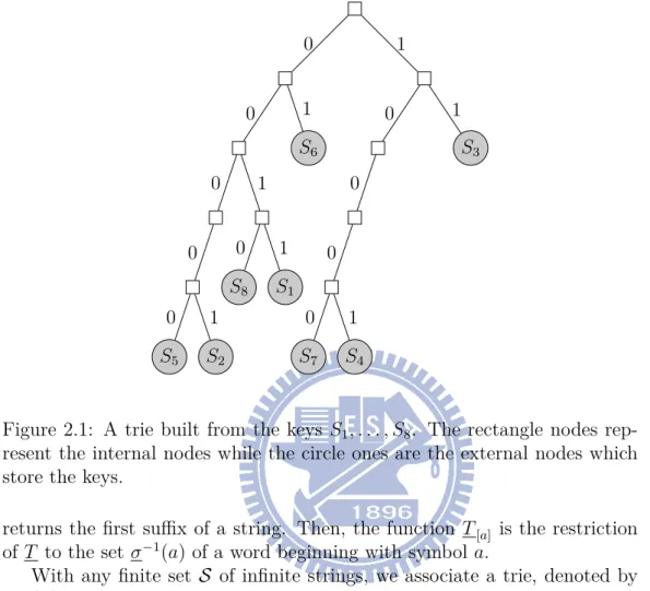
2.1 A trie built from the keys S1, . . . , S8. The rectangle nodes

rep-resent the internal nodes while the circle ones are the external nodes which store the keys. . . 10

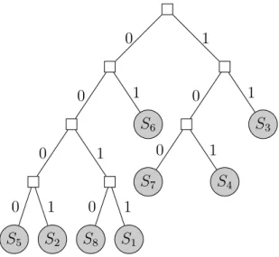
2.2 A PATRICIA trie built from the keys S1, . . . , S8. Note that

all the internal nodes have two childs.. . . 11

2.3 The process of building a DST from the keys S1, . . . , S8. Note

that if the order of the keys is diﬀerent, the resulting DST would be diﬀerent. . . 12

2.4 A bucket digital search tree built from the keys S1, . . . , S8 with

bucket size b = 2. . . . 13

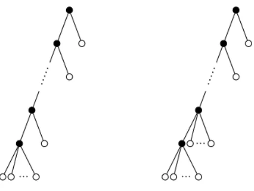
5.1 Two tries with internal nodes black and external nodes white. The trie on the left has all internal nodes of outdegree 2 except the last which is of outdegree i; the trie on the right has all internal nodes of outdegree 2 expect the last two which are of outdegree i. . . . 117

(12)

(13)

List of Tables

(14)

(15)

Chapter 1 Introduction

The word ”algorithm” is a distortion of the name of the 9th century Per-sian scientist, astronomer and mathematician Abu Abdallah Muhammad ibn Musa al-Khwarizmi. At al-Khwarizmi’s time, people used the term ”al-gorism”, which is also a distortion of al-Khwarizmi’s name, to refer to system-atic arithmetic methods which used Hindu-Arabic numerals to solve linear and quadratic equations. These methods appeared in a book written by al-Khwarizmi around the year 825 and the book was translated into Latin by the 18th century. The word ”algorithm” came from a Latin translation of al-Khwarizmi’s name.

The modern concept of algorithms was formalized in 1936 by A. Turing’s Turing machines and A. Church’s lambda calculus, which in turn formed the foundation of computer science. Although the formal deﬁnition of the term ”algorithm” remains a challenging problem up to date [151], it can be informally deﬁned as a step-by-step computational procedure which takes a set of values as input and produces a set of values as output [25].

Turing machine is the precursor of modern computers. Turing proved that such machines would be capable of performing any conceivable mathematical computation if it can be represented as an algorithm. With the computer rapidly becoming the most important tool in almost every aspects of people’s life, people started seeking more eﬃcient algorithms which make computers solve problems with less resources (time, storage spaces,…, etc.).

There are two different approaches to analyze the efficiency of an algo-rithm. The first one is to evaluate the performance of an algorithm in the worst-case senario. This kind of studies focus on the growth of resources an algorithm need in the worst-case. One of the major goals of such studies is to find an ”optimal algorithm” whose worst-case performance matches a ”lower bound” in the sense that any other algorithm for the same problem requires at least the same amount of resources in the worst-case scenario.

(16)

This approach was popularized by A. V. Aho, J. E. Hopcroft and J. D. Ull-man [4] and T. H. Cormen, C. E. Leiserson, R. L. Rivest and C. Stein [25]. P. Flajolet and R. Sedgewick use the term ”theory of algorithms” to refer to this type of studies [193].

The second approach, started by D. E. Knuth, is to study the average-case properties of algorithms. The average-case analysis works by ﬁrst construct-ing a suitable mathematical model for the input and then usconstruct-ing probabilistic, combinatorial and asymptotic methods to study the expected resource costs of the algorithm given an input drawn from the model. In [193], the authors described the goal of this approach as

....to be able to accurately predict the performance characteristics of particular algorithms when run on particular computers, in order to be able to predict resource usage, set parameters, and compare algorithms.

To design efficient algorithms and get a throughout understanding of them, both approaches are necessary. When a new algorithm appears, peo-ple need a rough idea of how the algorithm might perform and a rough comparison of this algorithm to other algorithms for the same problem. In such cases, the first approach will be an adequate choice. However, the first approach usually sacrifices many details and hence it provides less precision. Therefore, to acquire more specified information and make more accurate prediction of an algorithm, we need more details of the algorithm and the mathematical properties of the data structures manipulated by the algo-rithm. In such cases, the second approach plays an important role. Thus, a complete analysis of a specified algorithm should be a study which combines both approaches to get a full understanding of the algorithm. This leads to the emergence of the area ”analysis of algorithms”.

The electronic journal Discrete Mathematics and Theoretical Computer

Science deﬁnes ”analysis of algorithms” as follows:

Analysis of Algorithms is concerned with accurate estimate of complexity parameters of algorithms and aims at predicting the behavior of a given algorithm run in a given environment. It de-velops general methods for obtaining closed-form formulae, asymp-totic estimates, and probability distributions for combinatorial or probabilistic quantities, that are of interest in the optimization of algorithms. Interest is also placed on the methods themselves, whether combinatorial, probabilistic, or analytic. Combinato-rial and statistical properties of discrete structures (strings, trees,

(17)

tries, dags, graphs, and so on) as well as mathematical objects (e.g., continued fractions, polynomials, operators) that are rele-vant to the design of eﬃcient algorithms are investigated.

According to W. Szpankowski [202], the area of analysis of algorithms was born on July 27, 1963 when D. E. Knuth wrote his ”Notes on Open Addressing” on hashing tables with linear probing. In fact, using the term ”analysis of algorithms” to name the area was proposed by Knuth in his talk ”The Birth of the Giant Component” [63,105] given during the ﬁrst Average

Case Analysis of Algorithms Seminar in 1993. Knuth’s monumental series The Art of Computer Programming [125, 126, 127, 128] enriched this area and attracted many researchers devoting their eﬀort to develop it. After 50 years of development and with the contributions from many researchers, analysis of algorithms has became an area with much more abundant content. Nowadays, analysis of algorithms is a ﬁeld in the overlap of mathematics and theoretical computer science which enjoys close relations to discrete mathe-matics, combinatorial analysis, probability theory, analytic number theory, asymptotic analysis and complexity theory.

Analysis of algorithms is a fruitful area because of the helps from a wide range of mathematical tools. The development of analysis of algorithms also motivated researches about many diﬀerent areas in mathematics. The best example might be the emerging of analytic combinatorics.

The major goal of analytic combinatorics is to precisely predict the prop-erties of large structured combinatorial conﬁgurations, through an approach based comprehensively on analytic methods. It starts from an exact enumer-ative characterization of combinatorial structures by means of generating functions. Then, generating functions are viewed as analytical objects which map the complex plane into itself. Finally, techniques from complex analysis are used to derive asymptotic properties of the combinatorial objects from the generating functions.

The basic techniques and ideas of the theory of analytic combinatorics appeared quite early. Since the 18th century, many mathematicians, includ-ing L. Euler, A. Cayley, S. Ramanujan, G. Polya, and D. E. Knuth, have made contributions to the theory. However, systematic study of the theory started in 1960s by P. Flajolet because of the need from analysis of algo-rithms. As we have mentioned, combinatorial and statistical properties of discrete structures are major topics in analysis of algorithms. The need of mathematical tools for such topics fueled the development of analytic com-binatorics. In this thesis, we will use techniques from analytic combinatorics to study tree-based data structures.

(18)

graph theory. Moreover, they are also basic objects for data structures and algorithms in computer science. Take binary search trees as an example, which are a variant of the simplest tree structure, the binary trees, in graph theory. Since invented in 1960 in a joint work of A. S. Douglas, P. F. Windley, A. D. Booth, A. J. T. Colin and T. N. Hibbard [13,45,88,216], binary search trees became one of the most widely used data structures in computer science. Consequently, researchers began to study the properties of binary search trees. Started by Knuth [124], many diﬀerent methods, including classical combinatorics [17], probability theory [34] and analytic combinatorics [46], have been used in related researches.

The purpose of this thesis is to study another widely used tree-based data structure, the digital tree family. There are several outstanding books which introduce some aspects of digital trees [48, 139, 203]. However, many im-portant aspects of digital trees remain unknown and many problems are still unanswered. Our goal is to solve some of these problems and broaden related studies by introducing new ideas and using recently developed methods. For this purpose, we will ﬁrst review past researches and discuss the advantages and disadvantages of the known mathematical techniques which have been applied in previous studies. In the second half of this thesis, we will state our new results.

The chapters of this thesis are arranged as follows. Chapter 2 is meant to be a survey of known knowledge of digital trees. In this chapter, we first give the formal definition and the construction of digital trees. Then, we are going to explain the random model used in our studies. The final section of Chapter 2 is a collection of the majority of previous researches from the last several decades.

In Chapter 3, we are going to introduce the mathematical techniques which have been used in the study of random digital trees. These methods are from diﬀerent areas of mathematics, including analytic combinatorics, com-plex analysis, functional analysis and probability theory. For each method, we will give examples to illustrate how the method was applied to random digital trees.

We are going to show some new applications of the ”Poisson-Laplace-Mellin” method and Poissonized variance with correction in Chapter 4. The material of this chapter are from published papers by the author of this thesis and his collaborators. Section 4.1 is based on [78]. In this section, we will derive asymptotic expressions of mean and variance of approximate counting. Section 4.2 gives the expressions of the ﬁrst and second moment and the limiting distribution of the Wiener index of random digital trees. Results presented in this section are taken from [76, 77]. In Section 4.3, we are going to discuss a generalization of the Wiener index, the total Steiner

(19)

distance. To analyze this parameter, we will also discuss the k-th total path length. The results in this section are from [130].

The general topic of Chapter 5 is a framework for central limit theorems of certain shape parameters in random digital trees. In the ﬁrst two sections of this chapter, we state the framework which allows one to prove central limit theorems for shape parameters satisfying certain conditions. In the third section, we introduce a useful lemma which proves lower bounds for the variance of shape parameters and plays a key role in the framework. The rest of this chapter are examples of shape parameters which ﬁt into the framework. These results can be found in [77] and [79].

We conclude the thesis with a summary of the main achievement and some comments in Chapter 6.

(20)

(21)

Chapter 2 Random Digital Trees

2.1 The Origin and Applications of the

Ran-dom Digital Trees

Digital trees are an important class of random trees with numerous appli-cations in computer science. In this thesis, we are mainly dealing with four subclasses of digital trees, namely, Tries, PATRICIA Tries, Digital Search Trees (DSTs) and Bucket Digital Search Trees (b-DSTs).

Tries, first introduced by R. de la Briandais [29] and named by E. Fred-kin [72], are one of the most widely used data structure in computer science. Tries were created for retrieving data more efficiently. They turn out to be a huge success since they have many advantages over other already-existing data structures such as binary search trees. For example, looking up data in tries is faster in worst case comparing to binary search trees and the collision of different keys is avoided. Nowadays, tries are applied in many areas such as searching, sorting, dynamic hashing coding, polynomial factorizing, regu-lar languages, contention tree algorithms, automatically correcting words in texts, retrieving IP addresses and satellite data, internet routing and molec-ular biology. For a more detailed introduction and more references, see [167]. Several variants of Tries have been considered. One of them is PATRI-CIA Tries which were invented by D. R. Morrison [150] in 1986 (PATRICIA is an acronym which stands for Practical Algorithm To Retrieve Information Coded In Alphanumeric). D. R. Morrison proposed this data structure in order to avoid an annoying flaw of tries, namely, one way branching of inter-nal nodes. PATRICIA Tries share many advantages of Tries over balanced trees and binary search trees. Moreover, they require less space for stor-age. Because of this property, PATRICIA tries find particular application in the area of IP routing, where the ability to contain large ranges of values

(22)

with a few exceptions is particularly suited to the hierarchical organization of IP addresses. They are also used for inverted indexes of text documents in information retrieval.

Another variant of tries are digital search trees. They were first intro-duced by Coffman and Eve [24]. They have attracted considerable attention due to their wide applications, especially their close connection to the fa-mous Lempel-Ziv compression scheme [98]. The major difference between DSTs and Tries is that for DSTs, the data are stored in the nodes while the data only appears in the leaves of tries. Bucket digital search trees are a gen-eralization of DSTs, they are sometimes also called generalized digital search tree [90]. In b-DSTs, each node can store b keys. When b = 1, they corre-spond to the original DST. The advantage of such ”bucketing” is multifold such as reducing the root-to-node path lengths and improving the storage utilization. Because bucketing is an important tool in many algorithm de-signing problems ranging from hashing to computational geometry, b-DSTs are related to many practical algorithms [33,82,126,140,172]. For example, people use b-DSTs as a tool for memory management in UNIX [90].

General digital trees like tries, PATRICIA tries, DSTs and b-DSTs share a nice property, namely, the average height of the trees is almost optimal. This property ensures that the number of comparing operation during data searching is almost minimal.

There are a great deal of studies about all kinds of properties of digital trees. People study digital trees not only for the practical use we just dis-cussed but also the analysis of digital trees poses mathematical challenges. We will discuss the known properties and studies of digital trees in Section

2.3. However, before we do so, we will make precise the deﬁnition of the digital trees discussed above.

2.2 Random Model and Constructions for

Ran-dom Digital Trees

In this section, we will give the construction and random model for each variant of random digital trees. To make it easier to see the diﬀerences, we will always use the same set of inﬁnite binary strings as keys

S1 = 0011010 . . . S5 = 0000010 . . .

S2 = 0000110 . . . S6 = 0110101 . . .

S3 = 1110110 . . . S7 = 1000011 . . .

(23)

to build the examples in the following sections. We will use the same random model, the so-called Bernoulli model, for all the random digital trees we discuss in this thesis. For the Bernoulli model, it is assumed that the letters of each keys are generated independently.

In the binary case, the i-th key will be of the form

Ai,1, Ai,2, . . . , Ai,k, . . .

where for all 1_{≤ i ≤ n and j ∈ N, P(A}i,j = 0) = p andP(Ai,j = 1) = q = 1−p

with some 0≤ p ≤ 1.

For general m-ary cases, the i-th key is of the same form with Ai,j ∈ A =

{a1, . . . , am} for some alphabet A of the size m. Moreover, P(Ai,j = ak) = pk

for all 1_{≤ k ≤ m. Of course, we also have that}

m

∑

i=1

pi = 1 and 0≤ pi ≤ 1 for all 1 ≤ i ≤ m.

The Bernoulli model is the most simple model proposed. More realistic models have been propose by B. Valleé [206] and analyzed by Bourdon [14] and Valleé et. al. [23]. Although the Bernoulli model may seem too idealized for practical applications, typical behaviors under this model often hold under more general models such as Markovian or dynamical sources [96, 134,203].

2.2.1 Tries

Here we describe how to build a binary trie. For m-ary tries, the procedures are the same only the alphabet is expanded. We start with n data whose keys are infinite 0-1 strings. In a trie, the keys are only stored in the leaves. Whenever a new key is stored, we use it to search in the already existing trie by its prefix until we encounter a leaf which already contains a key. Then, the leaf is replaced by an internal node and the two keys are distributed to the two subtrees. If the two keys go to the same subtree, then the procedure is repeated until both keys go to different subtrees where they are stored in the leaves.

To make this definition more precise, we give a more formal description. Let {0, 1}∞ be the set of binary strings of infinite length, we define two operations. The map

σ :{0, 1}∞−→ {0, 1}

returns the ﬁrst letter of a string. The shift function

(24)

. ... . S3 . S6 . . S8 . S1 . S5 . S7 . S4 . S2 . 0 . 1 . 1 . 0 . 0 . 0 . 0 . 1 . 1 . 0 . 0 . 1 . 0 1 .. 0 . 0 . 1

Figure 2.1: A trie built from the keys S1, . . . , S8. The rectangle nodes

rep-resent the internal nodes while the circle ones are the external nodes which store the keys.

returns the ﬁrst suﬃx of a string. Then, the function T_[a] is the restriction of T to the set σ−1(a) of a word beginning with symbol a.

With any ﬁnite set S of inﬁnite strings, we associate a trie, denoted by

T R(S), deﬁned by the following recursive rules:

1. If _{S = ∅, then T R(S) is the empty tree.}

2. IfS = {s} has cardinality equal to one, then T R(S) consists of a single leaf node containing s.

3. If |S| ≥ 2, then T R(S) is an internal node represented generically by

2 to which 2 subtrees are attached

T R(S) =< 2, T R(T_[0]S), T R(T_[1]S) > .

2.2.2 PATRICIA Tries

PATRICIA tries are tries without one-way branching. As Figure 2.1 shows, tries may contain many internal nodes with only one child. To build a PA-TRICIA trie, one may build a trie ﬁrst and ”collapse” all the internal nodes

(25)

. ... . S3 . S7 . S4 . S6 . S8 . S1 . S2 . S5 . 0 . 0 . 1 . 0 1 _._. 1 . 0 . 1 . 0 ._. 1 0 . 1 . 0 . 1

Figure 2.2: A PATRICIA trie built from the keys S1, . . . , S8. Note that all

the internal nodes have two childs.

with only one child. To see the diﬀerence, compare Figure 2.1 and Figure

2.2.

Let P T R(S) be the PATRICIA trie associated to the ﬁnite set S of inﬁnite strings. P T R(S) is constructed by the following recursive rules:

1. If S = ∅, then P T R(S) is the empty tree.

2. If S = {s} has cardinality equal to one, then P T R(S) consists of a single leaf node containing s.

3. If _{|S| ≥ 2, by the number of distinct symbols contained in the multiset}

σ(S), there are two cases

(i) If σ(S) contains only one symbol, then

P T R(S) = P T R(T S).

(ii) Otherwise, T R(S) is an internal node represented generically by

2 to which 2 subtrees are attached

(26)

. . S1 . S1 . S2, S5, S6, S8 . S3, S4, S7 . S2 . S3 . S5, S8 S6 S4, S7 ... S1 . S2 . S3 . _S 4 . S7 . _S 6 . _S 5 . S8 . 0 . 1 . 0 . 0 . 1 . 1 . 0 . 0 . 0 . 1 . 1 . 1 . 0 . 0

Figure 2.3: The process of building a DST from the keys S1, . . . , S8. Note

that if the order of the keys is diﬀerent, the resulting DST would be diﬀerent.

2.2.3 Digital Search Trees

Here, we demonstrate how to build a binary digital search tree. As for tries and PATRICIA tries, we consider n keys which are inﬁnite {0, 1} strings. If

n = 1, then the only key is put in a node and the building process is ﬁnished.

Otherwise, we go through the following steps:

1. Store the ﬁrst key in a node (which will become the root of the tree). 2. Distribute the remaining keys into two sets according to the ﬁrst letter

of the key. If the ﬁrst letter is: 0: Put the keys to the left subtree. 1: Put the keys to the right subtree.

3. Remove all the ﬁrst letters of the keys in the subtrees. Build the sub-trees recursively according to the same rules.

For a bucket digital search tree with bucket size b, the building process is almost the same as for digital search trees. Only in step one of the con-struction, we put b keys in the node instead of only one node. It is easy to see the diﬀerences by comparing Figure 2.3 and Figure2.4.

(27)

. . S1, S2 . S5, S6 . S3, S4 . S8 S..7 0 . 0 . 1 . 0

Figure 2.4: A bucket digital search tree built from the keys S1, . . . , S8 with

bucket size b = 2.

2.3 Past Researches about Random Digital

Trees

Random digital trees have been studied from many different aspects. In this section, we focus on shape parameters of random digital trees. For each parameter, we will give the definition first and then explain the practical use of the parameter. We will also give a list of references of known results of the parameter.

Size

For random digital trees, the parameter size is the total number of internal nodes. So, this parameter is only relevant for tries and PATRICIA tries. People study this parameter because the number of internal nodes is pro-portional to the number of pointer needed to store the data structure. The less the number of internal nodes needed, the less the space required. Note that binary PATRICIA tries have a constant size and hence this parameter matters only for m-ary PATRICIA tries with m ≥ 3. For the study of size of tries, see [23, 39, 93, 103, 107, 109, 112, 116, 139, 145, 155, 95, 194]. For PATRICIA tries, see [14,15, 38, 39,146].

Depth

Depth is deﬁned as the distance from the root to a randomly selected node which normally contains data. Some researchers use the name depth of insertion or successful search time. It is one of the most well-studied pa-rameter since it provide a great deal of information for many applications. For example, the depth of a node storing a key represents the search time

(28)

for the key in searching and sorting algorithms [127]. Depth also gives the length of a conﬂict resolution session for tree-based communication proto-cols. For compression algorithms, depth is the length of a substring that may be occupied or compressed [7]. For the study of depth of tries, see [31, 36, 37, 57, 92, 97, 114, 136, 169, 192, 196, 198]. For the study of this parameter in PATRICIA tries, see [38, 39, 181]. Finally, for DSTs, see [36,135, 169, 176, 200, 139, 37, 30, 100, 102, 127, 113, 197].

Height

Height of a tree is the length of the longest path from the root to a leaf. It can also be understood as the maximum value of the depth. Height in digital trees reﬂects the the longest common preﬁx of words stored in a digital tree and is directly related to many important operations such as hashing in computer programming. See [23, 32,36,37,38,60,71,92, 168, 169,201] for studies of the height tries. See [36, 38, 39, 68, 111, 127, 168, 170, 171, 199, 201, 204] for PATRICIA tries and [122, 35,37, 47, 139, 169] for digital search trees.

Shortest path length

This parameter is the length of the shortest path from the root to the leaves. It was studied for tries by B. Pittel in [168,169]. He considered this parameter in order to derive the depth and height of a random trees.

Saturation level

Sometimes also called fill-up level. The levels of a tree are the set of nodes which are of the same distance from the root. The saturation levels are the full levels in a tree. Researcher have investigate the number of saturation levels, the maximum level which is full and so on. This parameter was firstly studied for the purpose of understanding the behavior of the parameter height [35]. However, it found also other applications in improving the efficiency of algorithms for IP address lookup problem [123]. For more details, see [35, 123, 169].

Stack size

In the deﬁnition of the height, every edge contributes one when counting the distance. Stack size is a kind of ”biased” height with the edges whose label is the last symbol in the alphabet (for binary case, the edges labeled by 1) make no contribution when counting the distance. For general m-ary tries and PATRICIA tries, if the order of the symbols in the alphabet is given,

(29)

a preorder traversals of the corresponding trie or PATRICIA trie gives the list of the words stored in the lexicographical order. When the traversal is implemented in a recursive way, the height measures the recursion-depth needed. However, in many cases the recursion is removed or a technique called end-recursion removal is used to save recursion calls. In those cases, the amount of memory space is no longer measured by the height and hence the parameter stack-size is introduced. For stack size of tries, see [16,157,158]. For the PATRICIA tries case, L. Devroye gave a method to compute this quantity in [39], however, without giving an explicit result.

Horton-Strahler number

The Horton-Strahler is defined similar to stack size for similar purposes. It specifies the recursion-depth needed for a traversal when pre-recursion removal is applied and the subtree is visited in an order chosen to minimize the recursion depth (this order is fixed for stack-size). Related study for tries can be found in [16, 41,156, 157, 158]. In [39], the author gave a bound for Horton-Strahler number of PATRICIA tries.

One-sided path length

One-sided path length is length of the path with all edges labeled by the same symbol. This parameter is directly related to a widely used algorithm called leader (or loser) selection. For the algorithm and its applications, see [59]. Because of its recursive nature, the algorithm will generate a tree which has a similar structure as tries during the selecting process. As as result, the one-sided path length of tries will directly reﬂect the eﬃciency of the algorithm. Related studies can be found in [59, 106, 174, 212, 214].

Occurrence of certain pattern

People may interested in nodes of the digital trees satisfying certain prop-erties or the number of certain speciﬁed subgraphs in a digital tree. For example, the so-called 2-protected nodes, the nodes which are neither the leaves nor parents of a leaf, is a type of nodes which has been studied. For more researches of this kind, see [60, 114, 116, 162, 192, 198, 169, 200, 89,

90, 98,114,121,127]

External path length

This parameter is the sum of distances between leaves and the root. In the case of trie data structures of hashing schemes, this parameter represents the

(30)

processing time in central unit. However, this parameter has drawn a lot of interests not because of its practical use but for an interesting phenomenon. It is easy to see that the mean of the external path length can be derived directly from the mean of the depth. Therefore, people expected that the variance of the external path length can also be directly derived from the variance of the depth. However, this is not the case [118]. This parameter has been studied for tries [94,99,119,167] and PATRICIA tries [14,39,118,199].

Internal path length

Internal path length is deﬁned as the sum of distances between internal nodes and the root. In contrast to tries and PATRICIA tries which store data in the leaves, digital search trees store data in the internal nodes. Thus, the internal path length can be seen as the counterpart of the external path length in digital search trees. L. Devroye studied this parameter for PATRICIA tries in [38]. Later, Fuchs, Hwang and Vytas gave a general framework for parameters with similar properties of the internal path length in [75]. Researches about internal path length of digital search trees can be found in [200,89,173,90,

117, 121, 98,192, 160, 74].

Distances

This parameter refers to the distance between two randomly selected nodes in a digital tree. It can be seen as a measure of how ”diverse” a tree is. R. Neininger studied this parameter to get better understanding of the Wiener index (which will be discussed later) of recursive trees [159]. After Neininger’s work, this parameter was studied for many diﬀerent classes of trees. For the study of distances of tries, see [1, 3, 22]. The study of distance of digital search trees can be found in [1,2].

Number of unary nodes in tries

Unary nodes are the nodes with exactly one child. PATRICIA tries are the tries with unary nodes ”collapsed”. Therefore, studying the number of unary nodes may gives us an estimation how much space is ”saved” in PATRICIA tries comparing to tries. Besides comparing the two variations of random digital trees, S. Wagner studied this parameter in [210] in order to get a better understanding of the eﬃciency of contention tree algorithms. Related studies can be found in [18, 205, 210]

(31)

Node proﬁle

The node profile of a random digital tree is a parameter which represents the number of nodes at the same distance from the root. This parameter has drawn a lot of attention because many fundamental parameters, including size, depth, height, shortest path length, internal path length and satura-tion level can be uniformly analyzed and expressed in terms of node profiles. Although node profile are of great importance, there are not too many re-searches about it until very recently. See [167] for the node profile of tries, [38,39] for node profile of PATRICIA tries and [48,50,129,135,51] for node profile of digital search trees.

Partial match queries

Multidimensional data retrieval is an important issue for the design of data base system. Partial match retrieval is a widely used method of retrieval which found many applications, especially in geographical data and graphic algorithm. For more detailed introduction of partial retrieval operation, see [65] and the references within. Because of the importance of this method, the performance of partial match retrieval on digital trees received a lot of interests. For the analysis of partial match retrieval on tries, PATRICIA tries and bucket-digital search trees, see [39,42, 65, 73,120,190,191].

Peripheral path length

This parameter was proposed by W. Szpankowski and M. D. Ward in [133,

211,213] with the name w-parameter. This parameter was originally applied in the study of Lempel-Ziv’77 data compression algorithm on uncompressed suffix trees. In [74], the authors renamed this parameter as the peripheral path length. The fringe-size of a leaf node is defined to be the size of the subtree rooted as its parent node. The peripheral path length is then defined to be the sum of the fringe-size of all leaves of the tree. Peripheral path length has been studied for tries, PATRICIA tries and digital search trees. For related researches, see [49, 74, 133, 211, 213].

Weighted path length

Let lj be the distance of the j-th node to the root and wj be the weight

attached to the j-th node, the weighted path length is deﬁned to be

Wn = n

∑

j=1

(32)

for a tree with n nodes. For many real life applications, people need to assign a weight to each edge or node of a graph. Weighted path length arises for these applications. For more details, see [74].

Diﬀerential path length

Also called the colless index, it inspects the internal nodes of trees. We partition the leaves descend end from internal nodes into two groups of sizes

L and R. The diﬀerential path length is the sum over all absolute values |L−R| for all ancestors. This parameter is investigated in the system biology

literature [11]. M. Fuchs et. al. studied this parameter for symmetric random digital search trees [74].

Type of nodes in bucket digital search trees

Because of the construction, a bucket digital search tree with bucket size

b ≥ 2 may have nodes containing diﬀerent number of keys. The authors of

[90] proposed a multivariate frame to study the number of each type of nodes in bucket digital search trees.

Key-wise path length

Since a node of a bucket digital search tree with b _{≥ 2 may contain more} than one key, the distance of two keys stored in a b-DST could be 0 in some cases. Therefore, researchers defined two different types of path length to study b-DSTs, wise path length and node-wise path length. The key-wise path length is defined as the sum of the distances between keys and the root. Related researches can be found in [74, 89].

Node-wise path length

Node-wise path length of b-DSTS is deﬁned to be the sum of all distances between nodes and the root. See [74,90] for more details.

(33)

Chapter 3 Related Mathematical

Techniques

3.1 Rice Method

Rice method, sometimes also called the Nörlund-Rice integral or Rice inte-gral, is named in honor of Niels Erik Nörlund and Stephen O. Rice. It is a fruitful method for ﬁnding the asymptotic expansion of sums of the form

n ∑ k=n0 ( n k ) (−1)kf (k). (3.1) The formulae of Rice integral is given by

n ∑ k=n0 ( n k ) (−1)kf (k) = (−1) n 2πi ∮ C f (z) n! z(z− 1) · · · (z − n)dz,

where C is a positive oriented closed curve encircling the points n0, n1, . . . , n

and f (z) is understood to be analytic within C. The integral can also be written as n ∑ k=n0 ( n k ) (−1)kf (k) = −1 2πi ∮ C B(n + 1,−z)f(z)dz,

where C is the contour mentioned before and B(a, b) is the beta function. Now we give a formal statement of the two formulaes.

(34)

[n0, +∞). Then, we have the representation n ∑ k=n0 ( n k ) (−1)kf (k) =(−1) n 2πi ∮ C f (z) n! z(z− 1) · · · (z − n)dz =−1 2πi ∮ C B(n + 1,−z)f(z)dz,

where C is a positively oriented closed curve that lies in the domain of an-alyticity of f (z), encircles [n0, n], and does not include any of the integers

0, 1, . . . , n0− 1.

Proof. The proof of these two equalities is omitted here since it is a simple

application of residue theorem. For the complete proof, see [69].

Suppose we have a ﬁnite diﬀerences sum of the form in (3.1), the Rice method allows us to compute an asymptotic expansion by the following steps:

Step 1. Extend f (k) which is originally deﬁned on integers to an appropriate

meromorphic function f (z).

Step 2. Choose a suitable contour C which encircles the points n0, . . . , n

and consider the Rice integral ∆ = (−1) n 2πi ∮ C f (z) n! z(z− 1) · · · (z − n)dz.

Step 3. Residue theorem yields that

∆ = n ∑ k=n0 ( n k )

(−1)kf (k) +{contribution from other poles inside C}.

Step 4. Estimate ∆.

Remark 1. The most diﬃcult step of the Rice method is usually Step 1.

Finding the meromorphic extension of f (k) is usually quite tricky. Also, to carry out Step 4 one needs growth properties of f (z), e.g. f (z) is of polynomial growth.

Rice method has been used in many researches about shape parameters of random digital trees. For example, P. Kirschenhofer, H. Prodinger and W. Szpankowski used it to derive the mean and variance of the internal path length of symmetric DSTs [114, 117, 121]. Here, we use the mean of the internal path length of DSTs as an instance to illustrate how the Rice method works.

(35)

We let Sn be the expectation of the internal path length of a symmetric

DST built on n strings. Then, under the Bernoulli mode, from the deﬁnition of the internal path length, we have the recurrence

Sn+1 = n + 21−n n ∑ k=0 ( n k ) Sk, (n≥ 0),

where the initial condition is given by S0 = 0. After some manipulations of

generating functions, we get that

Sn = n ∑ k=2 ( n k ) (−1)kQk−2.

Example 3.1.2. Consider the sum

Sn = n ∑ k=2 ( n k ) (−1)kQk−2, (3.2) where Qn = ∏n j=1(1− 2−j).

Step 1. We introduce the function

Q(s) = ∏ n≥1 ( 1− s 2n ) ,

then the constant Qn can be expressed as Qn = Q(1)/Q(2−n). Note

that Q(1) is ﬁnite and numerical results give us Q(1) ≃ 0.288788 · · · . Moreover, Q(1)/Q(22−z_{) is analytic on [2,}_{∞). Thus, we get the needed}

extension.

Step 2. We choose the contour C to be

{ z = x + iy : ( x− 1 2 )2 +y2 = N2, x≥ 1 2 } ∪ { z = x + iy : x = 1 2,−N ≤ y ≤ N } , and consider the integral

∆ = (−1) n 2πi ∮ C Q(1) Q(22−z₎ n! z(z− 1) · · · (z − n)dz.

(36)

Step 3. To compute the residues, we need to ﬁnd the poles of Q(1)/Q(22−z_).

The poles occur at z = 1+2kπi/ log 2 and hence the integral has a double pole at z = 1 and simple poles at z = 1 + 2kπi/ log 2 with k ∈ Z \ {0}. To compute the contribution from the double pole, we derive the series expansion (−1)nn! z(z− 1) · · · (z − n) = −1 z(z− 1) n ∏ j=2 ( 1− z j )₋₁ =− n z− 1− n(Hn−1− 1) + O(z − 1) and Q(1) Q(21−z₎ =Q(1) ∏ j≥0 ( 1− 2−(z+j))−1 =1− α(z − 1) log 2 + O((z− 1)2), where α =∑_n_≥1 1

2n₋₁. Combining the expansions, we get

Q(1) Q(22−z₎ (−1)n_n! z(z− 1) · · · (z − n) = ( 1 (z− 1) log 2 + 1 2 +O(z − 1) ) ×(1− α(z − 1) log 2 + O((z− 1)2)) × ( − n z− 1 − n(Hn−1− 1) + O(z − 1) ) . From the above expansion, we get the residue at z = 1 as

− n log 2(Hn−1−1)+n ( α− 1 2 ) =−n log₂n−n ( γ− 1 log 2 − α + 1 2 ) +O(1).

The poles at 1 + 2kπi/ log 2 with k _{∈ Z \ {0} make contributions δ(n)} [68], where δ(n) =− 1 log 2 ∑ k∈Z\{0} Γ ( −1 −2kπi log 2 ) e2kπi log2n_.

Step 4. On the right semi-circle, ∆ converges to 0 as n grows since

_Q(212−z₎

= O(1) as |z| → ∞.

On the left line, we have the bound O (∫ _∞ −∞ Γ(n + 1)Γ(1₂ + iy) Γ(n +1₂ − iy) dy ) =O(n1/2).

(37)

Combining all the above steps, we have Sn= n log2n + n ( γ − 1 log 2 − α + 1 2+ σ(n) ) +O(n1/2). (3.3) The internal path length of DSTs is not the only shape parameter which has been analyzed by the Rice method. For example, the external path length of tries and PATRICIA tries under the Bernoulli model can also be analyzed by the Rice method [118,119].

However, there are several other mathematical tools which can be used to analyze these shape parameters and they are sometimes more useful than the Rice method. In the following sections, we will introduce these tools. We begin with a standard tool which can transfer a problem under the Bernoulli model into a problem under the so-called Poisson model in which we have many useful tools to conquer the problem.

3.2 Poissonization and Depoissonization

In combinatorics and the analysis of algorithms, a Poisson version of a prob-lem (henceforth called Poisson model or poissonization) is often easier to solve than the original one, which we name here the Bernoulli model. Pois-sonization is a technique that replaces the original input by a poisson process. This technique was ﬁrst introduced by Marc Kac [108] in 1949. Recently, this technique ﬂourished in the community of analysis of algorithms and ran-dom combinatorial structures. See [99] for a comprehensive survey and many references.

We ﬁrst introduce the formal deﬁnition of analytical poissonization (which is also called Poisson Transform by G. Gonnet and J. Munro [83]).

Deﬁnition 3.2.1. Let {gn} be a sequence, then the Poisson transform ˜G(z)

of _{gn} is deﬁned as ˜ G(z) = e−z∑ n≥0 gn zn n!

for arbitrary complex z. ˜G(z) is also called the Poisson generating

func-tion.

If ˜G(z) is known, we can extract the coeﬃcient gn = n![zn] ˜G(z)ez.

How-ever, in most situations ˜G(z) satisﬁes a complicated functional/diﬀerential

equation that is diﬃcult to solve exactly. Fortunately, we have many tools, Mellin transform for example, to ﬁnd the asymptotic expansion of ˜G(z).

(38)

Therefore, the natural next step is to ﬁnd a method to derive asymptotic expansion of gn from the asymptotic expansion of ˜G(z). This step is called

analytical depoissonization. To explain the theory of analytical

depoissoniza-tion, we give some deﬁnitions ﬁrst.

Deﬁnition 3.2.2. (i) A linear cone is deﬁned as the region in the complex plane satisfying

Lθ ={z : | arg z| ≤ θ},

where _{|θ| ≤ π/2.}

(ii) A polynomial cone L(D, δ) is deﬁned as

L(D, δ) = {z = x + iy : |y| ≤ Dxδ_{, 0 < δ}_{≤ 1, D > 0}.}

We consider now a sequence _{gn}n≥0 and its Poisson generating function

˜

G(z) = e−z∑_n≥0gnzn/n!. Our goal is to derive the asymptotic expansion of

gn from ˜G(z). By Cauchy’s formula, we have

gn= n! 2πi ∮ _˜ G(z)ez zn+1 dz = n! nn_2π ∫ π −π ˜

G(neit) exp(neit)e−nitdt.

The depoissonization result will follow from the above by careful estimation of the integral using the saddle point method. Because the complete proof of depoissonization is rather long and technical, we omit it here. For the complete proof, see [99]. Here we only state the results.

Theorem 3.2.3. (Basic depoissonization lemma) Let ˜G(z) be the Poisson generating function of a sequence{gn} that is assumed to be an entire function

of z. Suppose that in a linear cone _Lθ both of the following two conditions

hold for some numbers A, B, R > 0, β and α < 1. 1. For z _{∈ L}θ and |z| > R | ˜G(z)| ≤ B|z|β; 2. For z _{̸∈ L}θ and |z| > R | ˜G(z)ez| ≤ Aeα|z|. Then, gn= ˜G(n) +O(nβ−1) for large n.

(39)

The above theorem can be generalized in several diﬀerent directions. In [99], the authors gave three generalized versions. Here we give the one which is most often used.

Theorem 3.2.4. (General depoissonization lemma) Consider a polynomial

cone L(D, δ) with 1/2 < δ ≤ 1. Let the following two conditions hold for some numbers A, B, R > 0 and α > 0, β and γ:

1. For z _{∈ L(D, δ) and |z| > R}

| ˜G(z)| ≤ B|z|βΨ(|z|),

where Ψ(z) is a slowly varying function, that is, a function for which for ﬁxed t, we have that limz→∞Ψ(tz)/Ψ(z) = 1;

2. For all z = ρeiθ _{with θ} _{≤ π such that z ̸∈ L(D, δ) and ρ = |z| > R}

| ˜G(z)ez| ≤ Aργeρ(1−αθ2). Then, for every nonnegative integer m

gn= m ∑ i=0 i+m ∑ j=0 bijniG˜(j)(n) +O(nβ−(m+1)(2δ−1)Ψ(n)) = ˜G(n) + m ∑ k=1 k ∑ j=1

bi,k+iniG˜(k+i)(n) +O(nβ−(m+1)(2δ−1)Ψ(n)),

where bij are the coeﬃcients of ex log(1+y)−xy at xiyj, that is

∑

i≥0

∑

j≥0

bijxiyj = ex log(1+y)−xy.

Let us take the external path length of tries, which has been mentioned at the end of Section 3.1 as an example. We denote by Pn the random variable

of the external path length of random tries built on n records. Then, under the Bernoulli model, we have

Pn d

= PBn+ Pn−Bn+ n, (n≥ 2), (3.4)

where Bn= Binomial(n, p) with p ∈ (0, 1) and P0 = P1 = 0. Let

˜ f (z) = e−z∑ n≥0 E(Pn) zn n!

(40)

be the Poisson generating function of the mean of Pn. Then from (3.4), we

get the functional equation ˜

f (z) = ˜f (pz) + ˜f (qz) + z(1− e−z). (3.5) One can now check by induction that ˜f (z) satisﬁes the assumptions of

The-orem 3.2.3 (see also Section 3.5.2 for a more systematic method of checking this). Then, this result implies that

E(Pn) = ˜f (n) +O(nϵ), (3.6)

where ϵ can be arbitrarily small. Thus, the natural next step is to ﬁnd more information about the asymptotic behavior of ˜f (z). For this purpose, we

introduce one of the most often used tools under such circumstance, the Mellin transform.

3.3 Mellin Transform

Mellin transform is the most popular integral transform in the analysis of algorithms. Its first occurrence is in a memoir of Riemann in which he used it to study the famous Zeta function. However, the transform gets its name from the Finish mathematician Hjalmar Mellin who did the first systematic study of the transform and its inverse. See [132] for a summary of his works. Nowadays, the Mellin transform is used in complex analysis, number theory, applied mathematics and analysis of algorithms. Apart from these applications in mathematics, the Mellin transform has also been applied in many different areas such as physics and engineering.

In the analysis of algorithms, the Mellin transform is mostly used to derive asymptotic expansions. The transform is deﬁned in the following:

Deﬁnition 3.3.1. Let f (z) be a function which is locally Lebesque integrable

over (0, +∞). The Mellin transform of f(z) is deﬁned by M [f(z); s] = f∗_{(s) =}∫ ∞

0

f (z)zs−1dz.

The largest open strip ⟨α, β⟩ in which the integral converges is called the

fundamental strip. To determine the fundamental strip, we have the following

lemma.

Lemma 3.3.2. If the function f (z) satisﬁes

f (z) =

{

O(zu_{), z} _{→ 0}+_;

O(zv_{), z} _{→ +∞,}

(41)

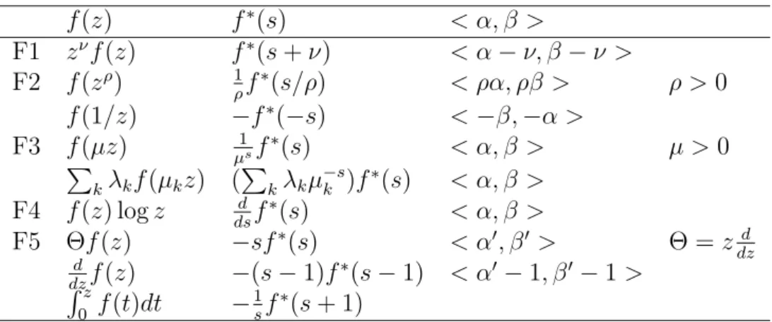
f (z) f∗(s) < α, β > F1 zνf (z) f∗(s + ν) < α− ν, β − ν > F2 f (zρ₎ 1 ρf∗(s/ρ) < ρα, ρβ > ρ > 0 f (1/z) −f∗(−s) <−β, −α > F3 f (µz)∑ _µ1sf∗(s) < α, β > µ > 0 kλkf (µkz) ( ∑ kλkµ−sk )f∗(s) < α, β > F4 f (z) log z _dsdf∗(s) < α, β > F5 Θf (z) −sf∗(s) < α′, β′ > Θ = z_dzd d dzf (z) −(s − 1)f∗(s− 1) < α′ − 1, β′− 1 > ∫z 0 f (t)dt − 1 sf∗(s + 1)

Table 3.1: Functional properties of Mellin transform

Before we start to develop a systematic theory of the Mellin transform, we give an easy example to show how the transform works.

Example 3.3.3. For f (z) = e−z, it is obvious that f (z) =

{

O(z0_), _z → 0+_;

O(z−b_{), z}_{→ +∞,}

where b is an positive real number which can be arbitrarily large. As a result, M [f(z); s] = Γ(s)

is deﬁned in _{⟨0, +∞⟩ and analytic there.}

Simple changes of variables in the deﬁnition of Mellin transforms yields many useful functional properties summarized in Table3.1.

Similar to other integral transformations, the Mellin transform has an inverse. For a given function f (z) and its Mellin transform f∗(s), we let

s = σ + 2πit and z = e−y. Then, the Mellin transform becomes a Fourier transform f∗(s) = ∫ _∞ 0 f (z)zs−1dz = ∫ _∞ −∞

f (e−y)e−σye−2πitydy =F [f(e−y)e−σy; t], where F [f(z); t] denotes the Fourier transform of f(z). As a result, the inversion theorem for the Mellin transform follows from the corresponding one for the Fourier transform. If ˆf (t) = F [f; t] is the Fourier transform,

then the original function is recovered by

f (z) =

∫ _∞

−∞

ˆ

(42)

Thus,

f (e−y)e−σy =

∫ _∞

−∞

f∗(σ + 2πit)e2πitydt.

Changing the variables y back to z, we get

f (z) = z−σ

∫ _∞

−∞

f∗(σ + 2πit)z−2πitdt.

Finally, by replacing σ + 2πit by s, we have

f (z) = 1

2πi

∫ c+i∞ c−i∞

f∗(s)z−sds.

Theorem 3.3.4. Let f (z) be integrable with fundamental strip ⟨α, β⟩. If c

is such that α < c < β and f∗(c + it) is integrable, then the equality 1

2πi

∫ c+i∞ c−i∞

f∗(s)z−sds = f (z)

holds almost everywhere. Moreover, if f (z) is continuous, then the equality holds everywhere on (0, +_∞).

As we mentioned before, the major application of the Mellin transform in the analysis of algorithms is to derive asymptotic expansions. This appli-cation comes from the correspondence between the asymptotic expansion of a function at 0 (and ∞), and poles of its Mellin transform in a left (resp. right) half-plane. Before we explain the correspondence, we introduce the singular expansion of a function.

Deﬁnition 3.3.5. Let ϕ(s) be meromorphic with poles in Ω. The singular

expansion of ϕ(s) is

ϕ(s)≍ ∑

s0∈Ω

∆(s; s0),

where ∆(s, s0) is the principal part of the Laurent expansion of ϕ around the

pole s = s0. Example 3.3.6. Given ϕ(s) = 1 s2_(s+1), since 1 s2_{(s + 1)} = 1 s + 1 +O(1) as s → −1 and 1 s2_{(s + 1)} = 1 s2 − 1 s +O(1), we have ϕ(s)≍ [ 1 s + 1 ] s=−1 + [ 1 s2 − 1 s ] s=0 .

(43)

With the help of the singular expansion of a function, we now give the correspondence.

Theorem 3.3.7. (Direct mapping) Let f (z) be a function with transform

f∗(s) in the fundamental strip ⟨α, β⟩.

(i) Assume that, as z _{→ 0}+_{, f (z) admits a ﬁnite asymptotic expansion of}

the form

f (z) = ∑

(ξ,k)∈A

cξ,kzξ(log z)k+O(zγ),

where −γ < −ξ ≤ α and the k′s are nonnegative. Then f∗(s) is

continuable to a meromorphic function in the strip _{⟨−γ, β⟩ where it} admits a singular expansion

f∗(s)≍ ∑

(ξ,k)∈A

cξ,k

(−1)kk!

(s + ξ)k+1, s∈ ⟨−γ, β⟩.

(ii) Similarly, assume that as z → +∞, f(z) admits a ﬁnite asymptotic expansion of the same form where now β _{≤ −ξ < −γ. then f}∗(s) is

continuable to a meromorphic function in the strip ⟨α, −γ⟩ where f∗(s)≍ − ∑

(ξ,k)∈A

cξ,k

(−1)k_k!

(s + ξ)k+1, s ∈ ⟨α, −γ⟩.

The direct mapping theorem gives a connection from the asymptotic ex-pansion of the function to the singular exex-pansion of the Mellin transform. Thus, the natural question is whether or not there is a way to get the asymp-totic expansion from the singular expansion. The answer is yes, when the Mellin transform is small enough at _{±i∞. More precisely, we have the} fol-lowing result.

Theorem 3.3.8. (Converse mapping) Let f (z) be continuous in [0, +∞)

with Mellin transform f∗(s) having a nonempty fundamental strip ⟨α, β⟩.

(i) Assume that f∗(s) admits a meromorphic continuation to the strip

⟨γ, β⟩ for some γ < α with a ﬁnite number of poles there, and is analytic on _{ℜ(s) = γ. Assume also that there exists a real number} η∈ (α, β) such that

(44)

when_{|s| → ∞ in γ ≤ ℜ(s) ≤ η. If f}∗(s) admits the singular expansion for _{ℜ(s) ∈ ⟨γ, α⟩,} f∗(s)≍ ∑ (ξ,k)∈A dξ,k 1 (s− ξ)k,

then an asymptotic expansion of f (z) at 0 is f (z) = ∑ (ξ,k)∈A dξ,k (−1)k−1 (k− 1)!z −ξ_{(log z)}k−1₊_O(z−γ_).

(ii) Similarly assume that f∗(s) admits a meromorphic continuation to

⟨α, γ⟩ for some γ > β and is analytic on ℜ(s) = γ. Assume also that

f∗(s) =O(|s|−r) with r > 1,

for η_{≤ ℜ(s) ≤ γ with η ∈ (α, β). If f}∗(s) admits the singular expansion

of the same form for ℜ(s) ∈ ⟨η, γ⟩, then an asymptotic expansion of f (z) at ∞ is f (z) =− ∑ (ξ,k)∈A dξ,k (−1)k−1 (k− 1)!z −ξ_{(log z)}k−1 +O(z−γ). Note that to apply Theorem 3.3.8, we need the condition

f∗(s) =O(|s|−r) with r > 1,

for s in a suitable strip. In other words, we need the Mellin transforms to be suﬃciently small along an vertical line. It is well-known that the small-ness of a Mellin transform is directly related to the degree of ”smoothsmall-ness” (diﬀerentiability, analyticity) of the original function. Here we introduce two theorems which are useful in determining the ”smallness” of the Mellin transforms.

Theorem 3.3.9. Let f (x)_{∈ C}r _{with fundamental strip} _{⟨α, β⟩. Assume that}

f (x) admits an asymptotic expansion as x→ 0+ _(x → ∞) of the form

f (x) = ∑

(ξ,k)∈A

cξ,kxξ(log x)k+O(xγ) (3.7)

where the ξ satisfy _{−α ≤ ξ < γ (γ < ξ ≤ −β). Assume also that each} derivative f(j)_{(x) for j = 1, . . . , r satisﬁes an asymptotic expansion obtained}

by termwise diﬀerentiation of (3.7). Then the continuation of f∗(s) satisﬁes

f∗(σ + it) = o(|t|−r) as |t| → ∞

(45)

Theorem 3.3.9 shows that smoothness implies smallness. The strongest possible form of smoothness for a function is analyticity. The following the-orem shows that the Mellin transform of an analytic function will decay exponentially in a quantiﬁable way.

Theorem 3.3.10. Let f (z) be analytic in a sector Sθ which is deﬁned as

Sθ ={z ∈ C|0 < |z| < ∞ and | arg(z)| ≤ θ} with 0 < θ < π.

Assume that for f (z) =O(|z|−α) as |z| → 0 in Sθ, and f (z) = O(|z|−β) as

|z| → ∞ in Sθ. Then

f∗(σ + it) =O(e−θ|t|) (3.8)

uniformly for σ in every closed subinterval of (α, β).

Note that a polynomial bound with positive power is enough for Theorem

3.3.8 while (3.8) provides an exponential bound. In fact, if the assumption

f∗(s) =O(|s|−r) with r > 1, in Theorem3.3.8 is replaced by

f∗(σ + it) =O(e−θ|t|),

we will get a stronger version of the converse mapping theorem as follows.

Theorem 3.3.11. Let f (z) be continuous in [0, +∞) with Mellin transform

f∗(s) having a nonempty fundamental strip ⟨α, β⟩.

(i) Assume that f∗(s) admits a meromorphic continuation to the strip

⟨γ, β⟩ for some γ < α with a ﬁnite number of poles there, and is analytic on _{ℜ(s) = γ. Assume also that there exists a real number} η∈ (α, β) such that

f∗(σ + it) =O(e−θ|t|), 0 < θ < π

when|t| → ∞ in γ ≤ ℜ(s) ≤ η. If f∗(s) admits the singular expansion

for _{ℜ(s) ∈ ⟨γ, α⟩,} f∗(s)≍ ∑ (ξ,k)∈A dξ,k 1 (s− ξ)k,

then an asymptotic expansion of f (z) at 0 is f (z) = ∑ (ξ,k)∈A dξ,k (−1)k−1 (k− 1)!z −ξ_{(log z)}k−1 +O(z−γ)

and the asymptotic expansion holds in the cone

(46)

(ii) Similarly assume that f∗(s) admits a meromorphic continuation to

⟨α, γ⟩ for some γ > β and is analytic on ℜ(s) = γ. Assume also that

f∗(s) =O(|s|−r) with r > 1,

for η≤ ℜ(s) ≤ γ with η ∈ (α, β). If f∗(s) admits the singular expansion

of the same form for _{ℜ(s) ∈ ⟨η, γ⟩, then an asymptotic expansion of} f (z) at ∞ is f (z) =− ∑ (ξ,k)∈A dξ,k (−1)k−1 (k− 1)!z −ξ_{(log z)}k−1₊_O(z−γ₎

and the asymptotic expansion holds in the cone

Sθ ={z ∈ C|0 < |z| < ∞ and | arg(z)| ≤ θ} with 0 < θ < π.

The advantage of asymptotic expansions holding in a cone in the complex plane is that asymptotic expressions of the derivative are obtained by term-by-term diﬀerentiation (the same is not true for asymptotic expansions which just hold on the real line). The justiﬁcation of this follows from a useful theorem due to J. Ritt [163].

Theorem 3.3.12. Let f (z) be analytic in an annular sector SR which is

deﬁned as

SR={z ∈ C|R < |z| < ∞ and θ1 < arg(z)≤ θ2} for some θ1, θ2 and 0≤ R.

If for some ﬁxed real number p, we have

f (z) =O(zp) (or f (z) = o(xp)) as z_{→ ∞ in S}R,

then

f(m)(z) =O(zp−m) ( or f(m)(z) = 0(xp−m)) as z_{→ ∞} in any closed annular sector properly interior to SR.

Now, with the knowledge of the Mellin transform, we can handle the functional equation (3.5). From the assumptions of Theorem 3.2.3 and the fact that P0 = P1 = 0, we have that

˜

f (z) =

{

O(z2_), _{as z}_{→ 0}+_,

O(z1+ϵ_{), as z} → ∞.

Now, applying the Mellin transform on (3.5), we obtain for_{ℜ(s) ∈ ⟨−2, −1−}

ϵ⟩

˜

f∗(s) = −Γ(s + 1)

隨機數位樹上加法性參數之機率分析

國立交通大學

應用數學系

博 士 論 文

隨機數位樹上加法性參數之機率分析

Probabilistic Analysis of Additive Shape

Parameters in Random Digital Trees

研 究 生:

李忠逵

隨機數位樹上加法性參數之機率分析

Probabilistic Analysis of Additive Shape

Parameters in Random Digital Trees

研 究 生：李忠逵

Student: Chung-Kuei Lee

指導教授：符麥克

Advisor: Michael Fuchs

國 立 交 通 大 學

應 用 數 學 系

博 士 論 文

隨機數位樹上加法性參數之機率分析

國立交通大學

應用數學系

摘要

Probabilistic Analysis of Additive Shape Parameters

in Random Digital Trees

Abstract

Contents

List of Figures

List of Tables

Chapter 1

Introduction

Chapter 2

Random Digital Trees

2.1 The Origin and Applications of the

Ran-dom Digital Trees

2.2

Random Model and Constructions for

Ran-dom Digital Trees

2.2.1 Tries

2.2.2

PATRICIA Tries

2.2.3

Digital Search Trees

2.3 Past Researches about Random Digital

Trees

Chapter 3

Related Mathematical

Techniques

3.1 Rice Method

3.2 Poissonization and Depoissonization

3.3

Mellin Transform

博士論文

研究生:

研究生：李忠逵

國立交通大學

應用數學系

博士論文