藉由最佳化LED排列方式增進背光源LED波長使用範圍之模型

(1)

i

國立交通大學

光電工程學系碩士班

碩士論文

藉由最佳化 LED 排列方式增進

背光源 LED 波長使用範圍之模型

Optimization of LED Arrangement for

Extending LED Binning Range in Backlight System

研究生：周秉彥

指導教授：黃乙白副教授

(2)

ii

藉由最佳化 LED 排列方式增進背光源 LED

波長使用範圍之模型

Optimization of LED Arrangement for

Extending LED Binning Range in Backlight System

研究生：周秉彥 Student：Ping-Yen Chou

指導教授：黃乙白 Advisor：Dr. Yi-Pai Huang

國立交通大學

光電工程學系碩士班

碩士論文

A Thesis

Submitted to Institute of Electro-Optical Engineering College of Electrical and Computer Engineering

National Chiao Tung University in Partial Fulfillment of the Requirements

for the Degree of Master in

Electro-Optical Engineering

July 2012

Hsinchu, Taiwan, Republic of China

(3)

i

藉由最佳化 LED 排列方式

增進背光源 LED 波長使用範圍之模型

碩士研究生：周秉彥指導教授：黃乙白副教授

國立交通大學光電工程學系碩士班

摘要

薄型化液晶電視(Slim format LCD-TV)逐漸成為顯示器市場趨勢，此外，因為發光二極體(LED)具有高能量萃取效率、較長使用壽命、不需使用含汞元素和符合綠色能源需求，LED 被視為是下一世代背光源的主流。基於製程上的因素影響，整面晶元(wafer)做出來的所有 LED，各項品質和參數會有些許不同，可以根據光波長、光強度和操作電壓來分類，然而，LED 在背光源的使用上，波長的挑選是非常苛刻的，導致目前面臨 LED 無法有效利用、背光源成本無法降低的問題。本篇論文提出一套分析背光源光學特性系統，來使 LED 能被運用的更有效率。這套系統的操作原理，首先，需要量測單一光源的光線擴散軌跡(Light spread function)與頻譜(spectrum)資訊，再藉由計算光輝度分布、頻譜線性疊加與色彩座標轉換的模擬程序，來獲得整面背光源色彩均勻性及色偏量的結果。此系統的準確度，已經由比對模擬結果與實際成品來獲得驗證，在展示品中，使用了外層螢光發光技術(Remote phosphor technology)，此結構具備厚度薄、壽命長和光源種類可用範圍廣的優點。藉此分析背光源光學特性系統，可輕易獲得不同條件下的背光色偏量，再加以設計可達降低生產成本與光源有效利用的目的。

(4)

ii

Optimization of LED Arrangement for

Extending LED Binning Range in Backlight System

Master Student: Ping-Yen Chou Advisors: Dr. Yi-Pai Huang

Institute of Electro-Optical Engineering

National Chiao Tung University

Abstract

Slim-format LCD-TV had been a trend for the current display market. Moreover, light-emitting diode (LED) is expected to become the backlight source of next generation, because of enhanced energy efficiency, a lager lifetime, the omission of mercury, and compliance with demand for green technologies. Since the manufacturing effect, LEDs are classified to different bin types by wavelength, brightness and voltage. However, the wavelength requirement of LED is very strict in backlight system. Therefore, LED cannot be used effectively in backlight systems, which still have high costs, currently.

In this thesis, an analysis method was developed to calculate the optical properties of direct-emitting backlight systems, which expands the usage of bins. The method based on computing the radiance distribution from the measured light spreading function and spectrum of LED. The calculation procedure includes linear spectral superposition and color difference evaluation. The accuracy of this method was verified by a real backlight module, which introduced the remote phosphor backlight system.

(5)

iii

This structure could have more benefits than the traditional one, including thinner thickness, longer life time, and wider LED bins. The conditions of acceptable color deviation values could be simply obtained, and the different binned LEDs could be efficiently used to reduce cost and achieve the wider binned-LEDs application purpose.

(6)

iv

誌謝

首先要感謝的是謝漢萍老師與黃乙白老師，在我碩班過程中予我的指導與訓練，包括研究的邏輯思考與組織報告的能力，以及提供良好的研究環境與資源，讓我順利完成論文，獲益良多。也感謝口試委員們在百忙之中蒞臨，並且不吝嗇地提出寶貴的建議，補足我思考上遺漏的地方。感謝洪健翔學長在研究上細心的指導與協助，在無數次的討論過程中給予我許多實用的意見。在專案合作方面，感謝日本 Sony 公司伊藤博士的協力與幫忙。實驗室的生活多采多姿，留下許多難忘的回憶。感謝芳正學長、國振學長、育誠學長、致維學長、志宏學長、台翔學長、韻竹學姐、柏全學長、奕智學長及精益學長的照顧，還有相同研究領域的姚順以及智清的切磋。一群同甘共苦的同學們，上翰、柏皓、哲軒、博凱、博鈞、綺文、書怡、岡儒以及白諭一起學習與成長的過程，更是我珍貴的回憶。有博元、又儀等其他學長姐和學弟妹們在課業與生活上的陪伴，研究上的辛苦與煩悶隨著歡笑聲而煙消雲散。另外，也感謝實驗室的助理們，為我們學生處理許多重要的事情。謝謝交大桌球隊的鄭鯤茂領隊、溫景財教練、游鳳芸教練和隊友們，交大光電的同學、學長姐和學弟妹們，系桌的隊友們，因為有你們，豐富了我的生活。最後感謝家人的支持與鼓勵，讓我無後顧之憂地完成學業。在此致上我最誠摯的感謝。

(7)

v

摘要 ... i

Abstract ... ii

誌謝 ... iv

Table of Contents ... v

Figure Captions ... vii

List of Tables ... xi

Chapter 1 ... 1

1.1 Liquid crystal displays (LCDs) ... 1

1.2 Direct-emitting backlight systems ... 3

1.3 Remote phosphor technology ... 5

1.4 Motivation and objective ... 7

1.5 Organization of this thesis ... 9

Chapter 2 ... 10

2.1 Geometrical optics in illumination system ...10

2.1.1 Law of refraction (Snell’s law)... 11

2.1.2 Law of reflection...12

2.1.3 Fresnel’s equations ...12

2.2 Radiometry ...14

2.3 Photometry ...16

2.4 Colorimetry ...19

2.4.1 CIE 1931 XYZ color space ...19

2.4.2 CIE 1976 LUV color space ...22

2.5 Summary ...24

Chapter 3 ... 25

(8)

vi

3.1.1 Light spread function (LSF) ...26

3.1.2 Binning factors and spectrums ...28

3.1.3 Gaussian binning distribution ...32

3.1.4 Convolution ...34

3.1.5 Comparing results ...34

3.2 Summary ...35

Chapter 4 ... 36

4.1 Accuracy of LSF approximation method ...36

4.1.1 Correctness of LSF superposition method ...37

4.1.2 Tolerance of self-fabricated module ...39

4.1.3 Affected color composition range of LED ...40

4.1.4 Built-in tolerance from bin width ...40

4.1.5 Boundary effect by light reflection ...42

4.1.6 Total difference between calculation and experiment...44

4.2 Summary ...45

Chapter 5 ... 46

5.1 Random arrangement ...46

5.1.1 Results of LEDs random arrangement: ...48

5.1.2 Discussion: ...55

5.2 Optimized arrangement ...56

5.3 Method for reducing gap ...60

5.4 Summary ...63

Chapter 6 ... 65

6.1 Conclusions ...65 6.2 Future works ...67

References... 68

Publication List ... 72

(9)

vii

Figure Captions

Fig. 1-1 Schematic configuration of a liquid crystal display. ... 2

Fig. 1-2 Schematic configuration of the conventional backlight systems. ... 3

Fig. 1-3 Schematic configuration of the conventional direct-emitting backlight systems. ... 4

Fig. 1-4 Scheme configurations of light emitting diodes. ... 6

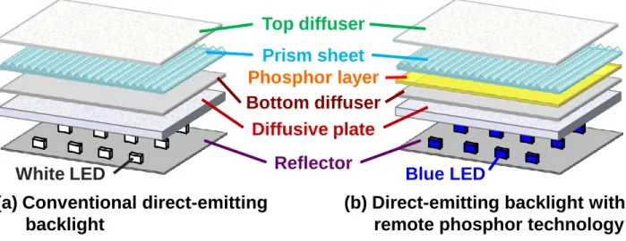
Fig. 1-5 Schematic configuration of (a) conventional direct-emitting backlight and (b) direct-emitting backlight with remote phosphor technology. ... 7

Fig. 1-6 Usable range of LED binning map for application in direct-emitting backlight. ... 8

Fig. 2-1 Reflection and Refraction on a boundary surface ... 11

Fig. 2-2 Defining geometry of radiometric quantities. ...15

Fig. 2-3 Scotopic and Photopic spectral sensitivities. ...17

Fig. 2-4 1988 CIE Photopic Luminous Efficiency Function ...18

Fig. 2-5 Color matching functions x( ) , y( ) , and z( ) in the CIE XYZ color system. ...20

Fig. 2-6 xy chromaticity diagram of CIE XYZ color system...21

(10)

viii

Fig. 3-1 Calculation model flowchart of backlight chromaticity. ...26

Fig. 3-2 Measurement setup of light spread function. ...27

Fig. 3-3 Light spread function of single LED illumination with phosphor. ...28

Fig. 3-4 CCD camera (ProMetric 1603F-1). ...28

Fig. 3-5 Spectral measurement of binned LED with phosphor film. ...29

Fig. 3-6 Different composed blue and yellow light in different locations. ...30

Fig. 3-7 Spectrometer (Topcon SR-UL1R). ...30

Fig. 3-8 Spectrums of blue LED with remote phosphor in different locations. ...31

Fig. 3-9 Spectrums of various binned-LEDs with remote phosphor. ...32

Fig. 3-10 Phosphor emission and excitation data...32

Fig. 3-11 Gaussian function with the waist (a)σ=2; (b) σ=4, and the ordinals of each bin. ...33

Fig. 4-1 Structures of simulated remote phosphor direct-emitting backlight model. ..37

Fig. 4-2 Ten inch direct-emitting prototype of (a) blue LEDs; and (b) phosphor sheet and optical films with LED illuminating. ...37

Fig. 4-3 Spectrums measurement setup with turning on (a) 3×3 LEDs; and (b) 5×5 LEDs. ...38

Fig. 4-4 Simulated spectrums superposition compared with measurement data. ...38

Fig. 4-5 Measurement deviation by small tilt angle between panel normal and detector. ...39

(11)

ix

Fig. 4-6 Peak wavelengths of LEDs in the same bin to test the built-in errors. ...41

Fig. 4-7 Prototype with white boundary. ...43

Fig. 4-8 Prototypes (a) without boundary; and (b) with black boundary. ...43

Fig. 4-9 Total differences between simulation and measurement in LUV color space. ...44

Fig. 4-10 Effected LEDs light by multi-reflection between reflector and diffuser plate. ...45

Fig. 5-1 Amount binned- LEDs of selecting LEDs exactly number method. ...47

Fig. 5-2 Amount binned- LEDs of picking up LEDs randomly method. ...47

Fig. 5-3 Color deviation with σ1=1 in selecting LEDs exactly method. ...49

Fig. 5-7 Color deviation with σ1=1 in picking up LEDs randomly method. ...51

Fig. 5-11 Color deviation with σ1=1 in the worst case. ...53

(12)

x

Fig. 5-15 Flowchart of the optimized arrangement method. ...56

Fig. 5-16 Optimized arrangement of each bin in basic unit array. ...57

Fig. 5-17 Arrangement of whole panel with considering boundary effects...58

Fig. 5-18 Optical films and illuminating prototype of optimized LEDs arrangement. 59 Fig. 5-19 Enhanced color uniformity of optimized arrangement than random arrangement with fixing (a) total wavelength range; (b) color deviation. ...59

Fig. 5-20 Simulated structures with (a) gap=30mm; and (b) gap=10mm. ...60

Fig. 5-21 Detected area of analyzed structure in Photometry. ...61

Fig. 5-22 Emitting light shapes of (a) normal LEDs (module gap=30mm); and (b) calculated LEDs (module gap=10mm). ...62

Fig. 5-23 Emitting light shape of real LEDs in the commercial when gap=30mm. ....62

Fig. 5-24 Emitting light shape of real LED in the commercial when gap=10mm. ...62

(13)

xi

List of Tables

Table 2-1 Radiometric units. ...14

Table 2-2 Photometric quantities...18

Table 2-3 Functions of applied principles...24

Table 4-1 Color difference between simulated superposition and measurement. ...39

Table 4-2 Color difference between different considered LEDs and measurement. ....40

Table 4-3 Color difference between two different wavelength LEDs in the same bin.41 Table 4-4 Built-in color errors by a width of peak wavelength in the same bin. ...42

Table 4-5 Color difference between the white boundary and black boundary modules. ...42

Table 4-6 Color accuracy of simulation and black / white boundary prototypes...44

(14)

1

Chapter 1 Introduction

During the past several decades, there has been rapid development of displays due to the advanced techniques. Slim format displays can be generally classified to different types basing on radiating methods, which are emissive and passive displays. Emissive displays include the organic light emitting diode (OLED), the plasma display panel (PDP), and the field emitting display (FED)[1,2,3]. One of the passive displays, liquid crystal display (LCD)[4], is the most popular slim format display. It should be noted, however, that there have been few attempts to describe a calculation method for the arrangement of color deviation and binned-LEDs, because of the complexities of the conventional ray tracing method. The main purpose of this thesis is to build an efficient calculation system of direct-emitting backlight to analyze the optical properties and color deviation.

1.1 Liquid crystal displays (LCDs)

In liquid crystal displays (LCDs), the liquid crystal (LC) acts as an electro-optic shutter which modulates the amount of incident light. Typical LCD configuration is shown in Fig.1-1, which consists of backlight, polarizer[5], thin film transistors (TFTs), LC layer, color filters, analyzer, and glass substrates. The backlight system is installed as hindermost device in LCD to provide a planar uniform light source. These may be cold cathode fluorescent lamps (CCFLs)[6] or light emitting diodes (LEDs)[7,8,9]. By polarizer absorbing one direction light, the non-polarized light is converted to a linear

(15)

2

polarization. The linear polarized light then propagates through the LC layer, which is placed between two glass substrates (e.g. indium tin oxide, ITO) and driven by a TFT to modulate the linear polarized light rotating angle. According to an absorbed direction of analyzer, the transmission in each pixel of the LCD can be defined as two types, normally white and normally black. The RGB color filter array is fabricated on the top glass substrate to mix the three monochromatic primary colors and produce full color images.

Fig. 1-1 Schematic configuration of a liquid crystal display.

Since the LC panel does not emit light by itself, a backlight system is required to provide illumination. Depending on the position of the light source, the backlight system can be classified into two types generally. One of them is called side-emitting backlight, as shown in Fig. 1–2 (a), when the light source is at the edge of a light guide

Backlight

Polarizer

TFT Glass

Color Filter

Analyzer

Glass

LC

Backlight

Polarizer

TFT Glass

Color Filter

Analyzer

Glass

LC

Active-matrix LCD

(16)

3

plate (LGP). And the other type is called direct-emitting backlight, as shown in Fig. 1–2 (b), when the light source is directly behind the LCD. A side-emitting backlight is typically used in small and middle-sized LCDs because of its small form factor and low power consumption. For example, it usually applied in mobile products since slim thickness and light weight. However, large-sized LCDs are more and more universal around human lives, such as LCD-TVs and electronic billboards. Since a display area is larger, an increased light source is needed to achieve the specified brightness. Compared with an edge-emitting one, direct-emitting LED backlight needs space for mixing light to maintain uniformity and has more benefits, such as application in larger-size LCD, local dimming technology and high-brightness display. Thus direct-emitting backlights are generally applied to large-sized LCDs.

(a) Side-emitting backlight (b) Direct-emitting backlight Fig. 1-2 Schematic configuration of the conventional backlight systems.

1.2 Direct-emitting backlight systems

The conventional direct-emitting backlight systems consist of a diffusive plate, optical films, and light sources, as shown in Fig. 1-2. The light sources, which are

(17)

4

CCFL lamps or LEDs, are arranged parallel behind the LC layer, as shown in Fig. 1-3[10]. A diffusive plate with diffusive particles inside the substrate is laid at a distance, which is called module gap, from the light source. After light is emitted from the light source, it spreads through module gap and diffused by the diffusive plate. The reflector is installed as a light recycle component in the bottom of whole device to reflecting the light which is mirrored by diffusive plate partially. A bottom diffusive sheet, with adjusted scattering ability, is applied to obtain a more uniform light distribution. Then the light propagates into a prism sheet to redirect spreading shape from a large inclined angle in the normal direction. Thus brightness can be enhanced in the normal viewing direction[11]. Finally, a top diffusive sheet is placed on top of the backlight system, which is applied to protect the micro-structure of the prism sheet and to reduce Moiré patterns[12]. Then the planar uniform light is outputted from backlight system.

(a) CCFL backlight (b) LED backlight Fig. 1-3 Schematic configuration of the conventional direct-emitting backlight systems.

Additionally, remote phosphor technology applied in backlight system will be introduced in the next section.

(18)

5

1.3 Remote phosphor technology

Remote phosphor technology is extensively applied in white LED illumination. According to its used functions, it can be classified to two applications, point light source and planar light source. In point light source application, remote phosphor technology mainly contributes to increase extraction efficiency and performed higher illuminating brightness when compared with conventional LEDs. In the other application, it mainly contributes to increase uniformity in planar light source.

Remote phosphor technology was firstly developed for LED packaging since Nadarajah’s research (2005)[13]

. A light-excited illuminating device configuring with external photo-fluorescent structure is so-called remote phosphor technology. The scheme of the conventional pcLED which utilizes a blue LED chip irradiating Cerium(III)-doped Y3Al5O12 phosphor[14] (YAG-phosphor) to obtain white light emission is shown in Fig.1-4(a). The broadband YAG-phosphor is coated on the LED die surface of a blue LED chip and packaged inside the whole device. This configuration has low efficiency because the diffuse phosphor directs 60% of total white light emission back toward the chip and leads losses of energy. Nadarajah et al. proposed the scattered photon extraction (SPE) pcLED[13,15,16,17] which contained a external YAG-phosphor. The external phosphor was coated on an external substrate outside the LED chips as shown in Fig. 1-4(b). Due to the separation of LED die and extraction of backward-emitted rays, the remote phosphor sheet system could convert the point light sources into a planar uniform light source and reduce the backlight thickness. Moreover, the efficiency of SPE pcLED was 61% higher than conventional pcLED.

(19)

6

(a) Conventional pcLED (b) Scattered photon extraction(SPE) pcLED Fig. 1-4 Scheme configurations of light emitting diodes.

Basing on research of the remote phosphor technology adopted pcLEDs, the direct-emitting backlight with remote phosphor technology is utilized in this thesis. Comparing with conventional direct-emitting backlight, the configuration with large-sized remote phosphor layers coated on flat substrates is shown in Fig.1-5. The phosphor layer is placed between optical films. After light spreading through module gap and diffusing by the diffusive plate, the point light source is converted into planar light source. Then the phosphor layer can be excited by planar blue light and emit yellow light to produce planar white light for backlight. Due to the backward scattering of excited yellow light, the direct-emitting backlight with remote phosphor technology has higher optical efficiency and uniformity than conventional direct-emitting backlight.

(20)

7

Fig. 1-5 Schematic configuration of (a) conventional direct-emitting backlight and (b) direct-emitting backlight with remote phosphor technology.

1.4 Motivation and objective

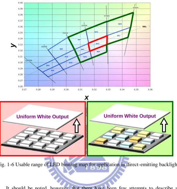
Both color uniformity of backlight system and cost down are key issues in LCDs fabrication. Moreover, LED is expected to become the backlight source of next generation, because of enhanced energy efficiency, a lager lifetime, the omission of mercury, and compliance with demand for green technologies. Since the manufacturing effect, LEDs are classified to different bin types by wavelength, brightness and voltage. However, the wavelength requirement of LED is very strict in backlight system. Fig. 1-6 shows a LED binning map[18], which represents the actual LEDs-bin classified range. From the LED binning map, only the center white bin LED can be chosen as light source in LED direct-emitting backlight. In the other words, the usable LEDs are rare in fabricating for backlight applications.

Reflector

Diffusive plate

Top diffuser

Prism sheet

Bottom diffuser

Phosphor layer

White LED

Blue LED

(a) Conventional direct-emitting

backlight

(b) Direct-emitting backlight with

remote phosphor technology

(21)

8

Fig. 1-6 Usable range of LED binning map for application in direct-emitting backlight.

It should be noted, however, that there have been few attempts to describe a calculation method for the arrangement of color deviation and binned-LEDs, because of the complexities of the conventional ray tracing method. The main purpose of this thesis is to build an efficient calculation system of direct-emitting backlight to analyze the optical properties and color deviation. By using the method, whether the phosphor having the wider blue LED binning range and evaluate the binning range under the required chromaticity uniformity or not is verified. According to this calculation system, an optimized binning distribution and arrangement method were proposed. In the last part, by applying the proposed method, the LED binning range for backlight could be extended thus becomes more cost effective.

y

x

(22)

9

1.5 Organization of this thesis

This thesis is organized as follows: The principles of backlight systems are presented in Chapter 2. In Chapter 3, the design concepts and processes of LSF approximation method are described. The simulation results and experimental results to analyze the accuracy of proposed method are verified in Chapter 4. In Chapter 5, the results of LEDs random arrangement, optimized arrangement, and reducing gap method are discussed. Finally, conclusions of this thesis and recommendations for the future work are presented in Chapter 6.

(23)

10

Chapter 2 Light Principles of Backlight Systems

For the purpose of designing and analyzing backlight systems, some optical principles are defined in this chapter. Emitted ray from light source propagates through an optical system, which is usually a homogeneous material, following the linear phenomena of light reacting. Thus geometrical optics is introduced to illustrate the light behavior in backlight systems. Moreover, results of the ray-tracing method can be mainly interpreted by Radiometry and Photometry. Furthermore, basing on the definition of Colorimetry, two color spaces, CIEXYZ and CIELUV, which specify color numerically, are also presented to explain the characterizations of phosphor films in this chapter.

2.1 Geometrical optics in illumination system

By electromagnetic theory and Maxwell equations, light exhibits a phenomenon as electromagnetic waves with time varying electric and magnetic fields when the wavelength of light is much smaller than surrounding objects it propagates through and around. After radiated from a point source, the light waves take a spherical form and travel in all directions. When propagating far away from the source, the light then behave like plane waves. The path of a hypothetical point on the wave front of light is called a ray of light. Thus the behavior of light can be approximated and described by ray optics (geometrical optics), including Snell’s law, Fresnel’s equation, and other optical principles.

(24)

11 2.1.1

Law of refraction (Snell’s law)

Snell’s law, also called law of refraction, defines the phenomenon of light refraction in the plane-of-incidence, which consists of an incident ray, a reflected ray, a refracted ray, and a normal direction of the surface. The verification of Snell’s law can be proved by Fermat’s Principle[19]. When a light ray having an angle i (the incidence

angle) with the surface normal strikes a boundary (interface) of two different optical media, it will induce a refracted ray transmitted through the boundary and makes a new angle t (the refraction angle) with the surface normal, as shown in Fig. 2-1. Based on

the definition of Snell’s law, the deviation of optical rays due to refraction is defined as the following equation[20],

sin

sin ,

i i t t

n





n



(2.1) where ni and nt are the refractive indices of the incident and transmitting medium,

respectively.

Fig. 2-1 Reflection and Refraction on a boundary surface

n

_i

n

_t

θ

_i

θ

_r

θ

_t

incidence

reflection

refraction

(25)

12 2.1.2

Law of reflection

In the plane of incidence, the propagating direction of the reflected rays follows below formula, which is also known as law of reflection[21]:

i r

 



(2-2) where i (incident angle) and r (reflected angle) are the angles of propagation

respectively. In other words, the reflected ray and the incident ray propagate with equal but opposite angle in the incident-of-plane of the same media.

2.1.3

Fresnel’s equations

Fresnel’s equations describe the energy of transmitted and reflected light at an interface between two different optical media. According to the polarization of light, electromagnetic waves can be classified to two types, P polarized light, and S polarized light, which vibrates parallel and perpendicular to the plane of incidence, respectively. The amplitude reflection and transmission coefficients r and t are respectively given by[22]:

cos

i i t t s i i t t

n

r

n









(2-3)

2 cos

cos

i i s i i t t

n

t

n







(2-4)

cos

t i i t p i t t i

n

r

n









(2-5)

2 cos

cos

i i p i t t i

n

t

n







(2-6)

(26)

13

where ni and nt are the refractive indices of the incident and transmitting medium, i and t are the angles made by the incident and refracted ray with the surface normal,

respectively.

According to radiant flux density (irradiance)[23], which unit is W/m2, the reflectance and the transmittance for polarized light are defined as:

2 s s

R



r

(2-7)

1

s s

T

 

R

(2-8) 2 p p

R



r

(2-9)

1

p p

T

 

R

(2-10)

where Rs and Ts are the reflectances and transmittances for S polarization light, and Rp

and Tp are the reflectances and transmittances for P polarization light, respectively.

According to the conservation of energy, the reflectance R and transmittance T of a random polarized light (eg. the nature light) striking the interface can be defined as the average of the polarized case as following equations:

2

s p

R





(2-11)

2

s p

T





(2-12) Basing on laws of reflection and refraction, the behaviors of light, reflected, and refracted, could be described by geometrical optics. Besides, by Fresnel’s equations, the reflectances and transmittances at an interface of two media could be calculated. Thus the energy of a particular light on the defined receiver could be obtained.

Therefore, the propagating direction of a light ray in an optical system can be traced and simulated to design and optimize the optical performances of the backlight

(27)

14 systems.

2.2 Radiometry

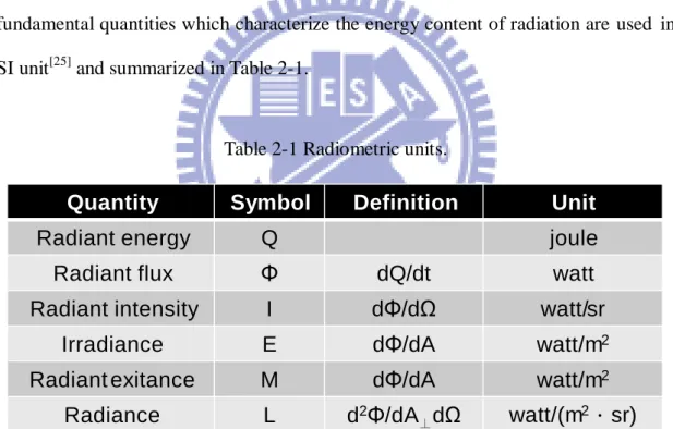
Radiometry is the science of measurement in electromagnetic radiation. It can gauge optical radiation within wavelengths ranging from 10 nm to 106 nm[24]. Consequently, the light source, which using ultraviolet-, visible-, and infrared-light, in optical systems can be analyzed by radiometry. Radiometric quantities include radiant energy, radiant flux, radiant intensity, irradiance, radiant exitance, and radiance. These fundamental quantities which characterize the energy content of radiation are used in SI unit[25] and summarized in Table 2-1.

Table 2-1 Radiometric units.

( t: time, : solid angle, A: area )

Radiant energy Q is the energy of a collection of photons (as in a laser plus). According to quantum mechanics, which classified by Albert Einstein, the energy of a single photon is hν. Radiant flux is defined as the measure of total power of radiation,

Quantity

Symbol

Definition

Unit

Radiant energy

Q

joule

Radiant flux

Φ

dQ/dt

watt

Radiant intensity

I

dΦ/dΩ

watt/sr

Irradiance

E

dΦ/dA

watt/m

2

Radiant exitance

M

dΦ/dA

watt/m

2

Radiance

L

d

2

_Φ/dA

(28)

15

which is the total emitted from a light source or the total debarkation on a particular surface. Basing on radiant energy Q and radiant flux , the other quantities are obtained by various geometric normalizations.

Radiant intensity I is generally used to describe the characteristics of sources whose size is infinitesimal, such as a point source. The definition of I is the radiant flux Φemitted per unit of solid angle Ω in a given direction of a specified surface, which the propagating radiation is incident passing through or upon, as shown in Fig.2-2 (a).

Irradiance E clarifies radiation distribution on a received plane. The definition is the radiant flux per unit area A of a specified surface, which the spreading radiation is incident on or passing though, as shown in Fig. 2-2 (b).

Fig. 2-2 Defining geometry of radiometric quantities.

Radiant flux dΦ

Solid angle element d

Ω

(a) Radiant intensity

Plane element dA

Radiant flux dΦ

(b) Irradiance

Plane element dA

Radiant flux dΦ

(c) Radiant exitance

θ

Plane element dA

dA

_⊥

=dAcosθ

Radiant flux dΦ

(d) Radiance

(29)

16

When the radiant flux leaving the plane per unit area A is considered, the term radiant exitance M is used instead of irradiance E. But the defined in the formulas are expressed by the same equation. Radiant exitance M clarifies radiation distribution on the plane which emits the radiation, as shown in Fig. 2-2 (c).

If an extended source, such as a planar source, is considered, radiance L is used to describe its characteristic. The definition of radiance L is the radiant flux Φ per unit project area A⊥ and per unit solid angle Ω of a specified surface, which the propagating radiation is incident on or passing through, as shown in Fig. 2-2 (d). The projected area of the plane element equals to dAcos, where  is the angle between the normal of the plane element and the direction of observation.

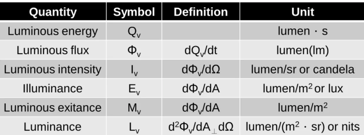
2.3 Photometry

Compared to Radiometry that describes all radiant energy, Photometry considers the responses to the optical radiation of human visual system, which are sensitivity at all wavelengths of visible light. Photometric quantity is an operationally defined quantity designed to represent the way in which the human visual system evaluates the corresponding radiometric quantity. The radiant power at each wavelength is weighted by CIE luminous efficiency curve, and the standard model that represents response or sensation of brightness for the eye versus wavelength is reproduced in Fig. 2-3. In particular, the optical radiation within the wavelengths range between 380 nm and 780 nm called visible light are discussed by photometry.

Photometric quantities include luminous energy, luminous flux, luminous intensity, illuminance, luminous exitance, and luminance. The definitions of photometric quantities are related to the corresponding radiometric quantities through the luminous

(30)

17

efficiency curve. The photometric quantities whose unit is based on lumen (lm)[25] are shown in Table 2-2. The unit lumen is defined as ‘luminous flux emitted into a solid angle of one steradian by a point source whose intensity is 1/60 of the intensity of 1 cm2 of a blackbody at the temperature of platinum (2042K) under a pressure of one atmosphere.’

Fig. 2-3 Scotopic and Photopic spectral sensitivities.

From the definition of lumen, the corresponsive maximum spectral efficiency of human eyes, which one watt is equal to 680 lumens, is at the wavelength 555 nm. Thus, the luminous flux v emitted from a source with a radiant flux λλ  is given by:

( )

683 lm/w

( )

v



V



 

d











(2.3) where  is the wavelength and



V_( ) is the normalized luminous efficiency function depicted in Fig. 2-4[26].

(31)

18

Table 2-2 Photometric quantities.

(t: time, : solid angle, A: area)

Fig. 2-4 1988 CIE Photopic Luminous Efficiency Function

Quantity

Symbol

Definition

Unit

Luminous energy

Q

v

lumen．s

Luminous flux

Φ

_v

dQ

_v

/dt

lumen(lm)

Luminous intensity

I

_v

dΦ

_v

/dΩ

lumen/sr or candela

Illuminance

E

v

dΦ

v

/dA

lumen/m

2

or lux

Luminous exitance

M

_v

dΦ

_v

/dA

lumen/m

2

(32)

19

2.4 Colorimetry

Colorimetry is the science designing and quantifying color comparison and matching in human eyes. As mentioned in prior paragraph, the photometric quantities have provided measures to describe the amount of energy for visible light, where the optical radiations within wavelengths range from 380 nm to 780 nm. However, in human visual system, the optical radiations stimulate not only intensity response (brightness) but also chromatic response (chromaticity). In human eyes, the retina contains two major types of light-sensitive photoreceptor cells used for vision: the rods and the cones, which are responsible for low-light monochrome vision and for color vision, respectively. Therefore, colorimetry is imported to specify the chromatic performance of backlight units in this thesis. The CIE 1931 xyY and CIE 1976 LUV color spaces, which have been developed for denoting colors numerically, are described in the following paragraphs.

2.4.1

CIE 1931 XYZ color space

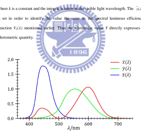
The CIE 1931 XYZ system, created by the International Commission on Illuminance (CIE, Commission internationale de l'éclairage) in 1931, is one of the first mathematically defined color systems that quantify colors numerically[27]. The human eye has three types of cones that perceive for short (S), middle (M), and long (L) wavelengths light, often referred to as red, green, and blue, respectively. Accordingly, in definition, three parameters are used to describe a color sensation. The tristimulus values of a color are the amounts of three primary colors in a three-component additive color model, which is needed to match that test color[28]. In the CIE 1931 XYZ system, the tristimulus values are called X, Y, and Z. The tristimulus values for a color with a

(33)

20

stimulus Ψ(λ ) can be evaluated from the color matching functions, the numerical illustration of the chromatic response of standard observer[29] (see Fig. 2-5), according to the following equations:

( ) ( )

vis

X



k







x

 

d

_(2.4)

( ) ( )

vis

Y



k







y

 

d

_(2.5)

( ) ( )

vis

Z



k







z

 

d

_(2.6)

where k is a constant and the integral is taken in the visible light wavelength. The y( ) is set in order to identify the value the same as the spectral luminous efficiency function Vλ() mentioned earlier. Thus the tristimulus value Y directly expresses a

photometric quantity.

(34)

21

Fig. 2-6 xy chromaticity diagram of CIE XYZ color system.

Basing on CIE 1931 XYZ system, a color could be represented by applying the tristimulus values X, Y, and Z in a three-dimensional color space, called CIE 1931 XYZ color space. Besides, for convenient descriptions of colors, a color space represented by x, y, and Y, known as CIE 1931 xyY color space, was evaluated[30]. In this color space, the x and y are defined as following equations:

X

x

X

Y

Z



 

(2.7)

Y

y

X

Y

Z



 

(2.8)

1 Z

z

x

y

X

Y

Z



  

 

(2.9)

(35)

22

where z coordinate could be neglected by providing Y parameter which is a measured value of the luminance of a color. Therefore, the chromaticity description of a color could be expressed more conveniently in a two-dimensional plane, which is called CIE xy chromaticity diagram and be widely used in custom (see Fig. 2-6).

However, the xy chromaticity diagram is highly non-uniform and has been found to be a serious problem in custom[31]. The color difference between two colors could not be calculated by using CIE 1931 XYZ color space or xy chromaticity diagram. Therefore, a uniform color space, the CIE 1976 LUV color space, is proposed to replace the non-uniform CIE 1931 XYZ color space.

2.4.2

CIE 1976 LUV color space

The CIE 1976 LUV color space proposed by CIE in 1976, which is an approach to define an encoding with uniformity in the perceptibility of color difference[32]. This uniform color space is based on a simple-to-compute transformation of the CIE 1931 XYZ color space[33.34]. For the non-linear relations from CIE 1931 XYZ color space to CIE 1976 LUV color space, the three-dimensinal orthogonal coordinates adopted in CIE 1976 LUV color space are defined as follows[35]:

1/3

*

116(

/

_n

)

16 L



Y Y



(2.10)

*

13 *( '

n

')

u



L

u



u

(2.11)

*

13 *( '

n

')

v



L

v



v

(2.12)

where u’ and v’ is the coordinates of two-dimensional u’v’ chromaticity diagram (see Fig. 2-7), which is used similarly to xy chromaticity diagram, defined as Equation 2.13 and 2.14. Yn, un’, and vn’ are the tristimulus value and the chromaticity coordinates u’

(36)

23 and v’ of reference white, respectively.

4 '

4

15

3 X

u

X

Y

Z





(2.13)

9 '

15

3 Y

v

X

Y

Z





(2.14)

Basing on the uniform CIE 1976 LUV color space, the color difference of two colors could be calculated simply and directly without changing based domain. The color difference u’v’ between two colors (u1’,v1’) and (u2’,v2’) at the u’v’ chromaticity

diagram is defined as[36]: 2 2 2 2 1 2 1 2

' '

(

')

(

')

(

'

')

(

'

')

u v

u

v

u

v







 









(2.15)

In this thesis, Equation 2.15 is imported to judge the chromatic performance of the backlight units.

(37)

24

2.5 Summary

Table 2-3 summarizes the principles mentioned earlier in this chapter. In this thesis, ray-tracing method was used to explain properties of light spread function (LSF). By Snell’s law, law of reflection, and Fresnel’ equations, the propagation trajectory and the carried energy of light could be calculated. Besides, basing on radiometry and photometry, the wavelength-corresponded spectrums with different detected locations of backlight illustrated the compositions of emitted (blue) and stimulated (yellow) light. Furthermore, the flux and chromaticity distribution of the backlight can be simulated by the numerical superposition in commercial calculated software, MATLAB. Accordingly, the CIELUV color space and the color difference u’v’ were utilized to judge the optical performances of the backlight units, which are the most important part for developing simulation models of backlight system. Therefore, the measurement framework will be discussed in the following chapter.

Table 2-3 Functions of applied principles.

Method

Principle

Function

Ray tracing

Snell’s law

Calculating propagation

trajectory and carried energy

of light.

Law of reflection

Fresnel’s equations

Radiometry

&

Photometry

Light flux properties

Characterizing light

scattering properties of

phosphor films.

Photopic spectral sensitivity

Colorimetry

CIE LUV color space

Specifying chromaticity

performance of backlight

output distribution.

Color difference (Δu’v’)

(38)

25

Chapter 3 Concept of LSF Approximation Method

The purpose of this thesis is to extend the blue LED binning range for remote phosphor backlight system. The first step is to build an accurate calculation model for the system. Here the chromaticity and luminance uniformity of the phosphor can be effectively calculated by the spectral distributions of the different binned LEDs under the considered configuration. As the structural parameters, including the pitch, gap, and optical films, are defined, the light spreading function (LSF) by single LED is measured first. Therefore, we can calculate the chromaticity distribution of the backlight by the numerical superposition of the LSF against the conventional ray-tracing computation.

3.1 LSF approximation method

The LSF approximation method was built to analyze the optical property and color uniformity of backlight system before manufactured process in a factory. Here the procedures of calculated method could be summarized to the flowchart in Fig. 3-1. Based on the calculation of LSF approximation method, a color deviation of a backlight could be computed and controlled less than the required light flux and chromaticity uniformity by choosing acceptable binning ranges, which are defined by wavelength, flux, and Vf. Moreover, by designing and optimizing binning distribution and arrangement, the more outer binned-type and binned-ratio of LEDs could be chosen to use in LCD backlights. In other words, according to this calculation system, the LEDs information of a good enough color uniformity backlight, which Δu’v’ less

(39)

26

than an acceptable value of color deviation, were evaluated by the simulation.

Fig. 3-1 Calculation model flowchart of backlight chromaticity.

3.1.1

Light spread function (LSF)

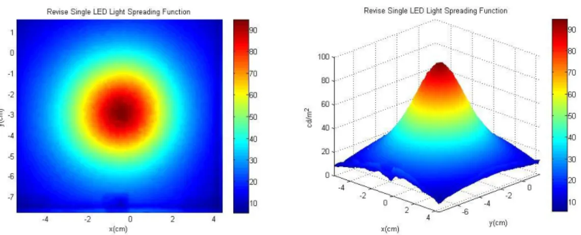
The first step of the procedure was to measure the light spread function (LSF)[37] of the backlight system module under single LED illuminating. The measurement setup was shown as Fig. 3-2. Since the LSF would be changed with the varying LED, module gap and optical films, the parameters should be defined before measuring it. Therefore, the measured LSF completely characterized the parameters of the backlight system configuration.

In a case of this thesis analyzing, the gap of module is 30 millimeter, and the encapsulation style of LED, whose driving voltage is about 3.2 V, is a bare chip made by Everlight Electronics CO., LTD. Besides, the optical films from bottom to top are diffuser plate, phosphor sheet, which is also called PEBBLE made by Sony CO.,

LSF

P

_(n,m)

(l)

I

_(n,m) Gaussian Binning Distribution (wavelength) Random Arrangement CIELUV Convolution Δ u’v’< Acceptable Deviation Value Acceptable Results

Y

N

Change distributing factor

Gaussian Binning Distribution

(intensity)

Binning Factors

(40)

27

diffuser sheet, BEF and DBEF, sequentially. Under these conditions, the LSF of single LED (Fig. 3-3) was measured by CCD camera (ProMetric 1603F-1)[38], as shown in Fig. 3-4. Since the LSFs are similar under the same encapsulation style of LED and module structure, this step of procedure could be just measured once, and the result indicates to represent LSF of every LED. According to the measured data of LSF, a intensity affected weight of LED in every backlight location could be obtained, and the flux uniformity of backlight system can be superposed. Furthermore, considering the difference of color composition in varied binned-LEDs, the color deviation of backlight system could be calculated, which are described in the following paragraphs.

Fig. 3-2 Measurement setup of light spread function.

Blue LED Array

Phosphor Sheet

(41)

28

Fig. 3-3 Light spread function of single LED illumination with phosphor.

Fig. 3-4 CCD camera (ProMetric 1603F-1).

3.1.2

Binning factors and spectrums

After the LSF measurement, the spectral distribution of the various binned LEDs with the considered phosphor film would be measured. Fig. 3-5 illustrates the measurement setup. The spectral distributions were varied with the different binned LEDs, so the relative spectrums[39] represented the binning factors.

(42)

29

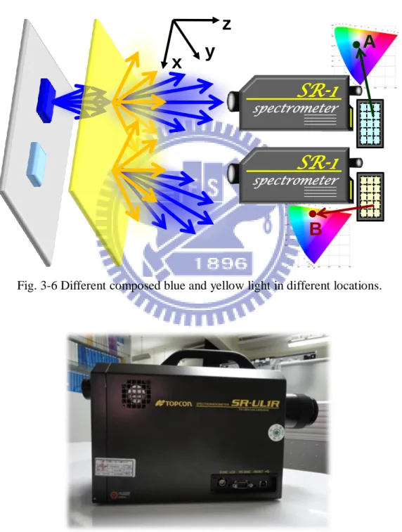
Fig. 3-5 Spectral measurement of binned LED with phosphor film.

It is worth noting that the spectral radiance has varied composition on different locations and viewing angles. It’s caused from the diverse angular radiance distributions of the excitation and emission light. The phosphor-scattered blue light has higher directivity than the phosphor-emitted yellow light, so there is the color dispersion pattern of measured LSF, as shown in Fig. 3-6.

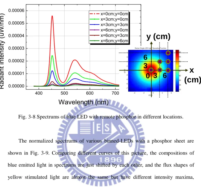
In this section, spectrums measured by spectrometer (Topcon SR-UL1R[40], see Fig. 3-7) are shown in Fig. 3-8 and Fig. 3-9 with the same conditions in the prior LSF section. According to principles of remote phosphor technology, a spectrum could be analyzed and classified to two parts: one is short wavelength range, which composing the blue light emitted by LED, and the other is long wavelength range, which consisting of yellow light stimulated by phosphor sheet.

Fig. 3-7 shows measured spectrums with the same LED and phosphor sheet in the different locations of backlight system. By normalizing the maximum intensity of spectrums, when a distance with the location above LED is farther, the intensity ratio

(43)

30

of yellow light divided by blue light in spectral configuration is higher. This phenomenon occurs by different field shapes of emitted blue light and stimulated yellow light. Since field shapes of blue light and yellow light are directional and lambertian, respectively, the blue component is higher than yellow one in normal detection, as mentioned in the previous paragraph.

Fig. 3-6 Different composed blue and yellow light in different locations.

Fig. 3-7 Spectrometer (Topcon SR-UL1R).

x

y

z

A

SR-1

spectrometer

SR-1

spectrometer

B

(44)

31

Fig. 3-8 Spectrums of blue LED with remote phosphor in different locations.

The normalized spectrums of various binned-LEDs with a phosphor sheet are shown in Fig. 3-9. Comparing different curves of this picture, the compositions of blue emitted light in spectrums are just shifted by each other, and the flux shapes of yellow stimulated light are almost the same but have different intensity maxima, which can be explained by phosphor emission and excitation data, as shown in Fig. 3-10. Based on phosphor materials, a phosphor sheet composed red and green stimulated light[41], which is made by Sony CO., is chosen for the better color rendering index. The dashed lines indicate the phosphor sheet absorptive ability in different wavelengths of blue LEDs, which is proportional to the maximal excitations of red and green light. Besides, the solid lines illustrate the spectral distribution of red and green emissive light.

400 500 600 700 800 0.00000 0.00001 0.00002 0.00003 0.00004 0.00005 0.00006 x=0cm;y=0cm x=3cm;y=0cm x=3cm;y=3cm x=6cm;y=0cm x=6cm;y=3cm x=6cm;y=6cm

Wavelength (nm)

R

a

d

ia

n

t in

te

n

si

ty (

u

W

/n

m

)

x

(cm)

y (cm)

0 3

3

6

(45)

32

Fig. 3-9 Spectrums of various binned-LEDs with remote phosphor.

Fig. 3-10 Phosphor emission and excitation data.

3.1.3

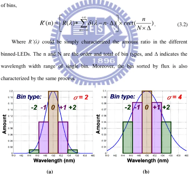
Gaussian binning distribution

The effect of chromaticity uniformity in the backlight system would be strongly affected by the LED binning distribution, which be sorted by wavelength and flux. In Fig. 3-11 (a) and (b), the discrete curve represents the practical wavelength bin

0 10 20 30 40 50 60 350 400 450 500 550 600 650 700 750 Wavelength (nm) In te n si ty ( a. u .) SP-G1-Ex SP-G1-Em SP-R2-Ex SP-R2-Em G-excitation G-emission R-excitation R-emission

(46)

33

distribution, including 0th, ±1st and ±2nd bin types. This discrete distribution is described by the applied Gaussian function[42],

 





_









_





_







0₂2 5 . 0

2 exp

2

1 )

(











R

_{, (3.1)}

where R(λ) is bin distribution sorted by wavelength λ. The ₀ symbol defines the peaked wavelength in the standard bin. And the waist of the Gaussian function σ indicates the width of this bin distribution. Since the Gaussian function, R(λ), is continuous, it should be convolution with the comb function to transform into the discrete one, and be multiplication with the rectangular function to limit the range width of bins,

)

(

)

(

)

(

)

(

'





























  

N

n

rect

n

R

n

R

n







_{. (3.2)}

Where R’(λ) could be simply characterized the amount ratio in the different binned-LEDs. The n and N are the order and total of bin types, and Δ indicates the wavelength width range of single bin. Moreover, the bin sorted by flux is also characterized by the same process.

(a) (b)

(47)

34 3.1.4

Convolution

Basing on the normalized LSF, the luminance distribution of the LED array with phosphor would be summed by the superposition,











     s t y x t s t s P x sp y tp L y x LSF y x L( , ,



) ( , )* ₍ _,₎ ₍ _,₎(



)



( , ) , (3.3)

where the weights P(s.t) and I(s.t) of the sampling function (x-spx, y-tpy) are the spectral

binning factors (normalized spectral distribution) and flux binning factors (maximum luminance of the LSF obtained from binned LED) varied with the LED position (s,t). The spectral radiance distribution at any point (x, y) on the phosphor emission surface could be obtained by this function, which is defined as spatially spectral distribution.

3.1.5

Comparing results

The chromaticity distribution of the backlight system module at the considered position could be transformed from the spatially spectral distribution function by the definition of the CIELUV color space. The evaluating factor is defined as

2 2 ) , (st



(

u

'

(

x

s

,

y

t

)



u

'

e

)



(

v

'

(

x

s

,

y

t

)



v

'

e

)



, (3.4)

where the (s, t) indicates the position exactly above the LED at the s-th line and t-th row. Here the data were compared with the expected value. One set of the calculated results would be verified with the experimental measurement of a small-size prototype.

(48)

35

3.2 Summary

To develop a simulation model to test color deviation of backlight system and design an acceptable binned distribution, the backlight configurations, which were integrated a direct-emitting backlight with the remote phosphor technology, were first specified. In the LSF approximation method, a CCD camera measured LSF completely characterized the conditions of LED encapsulation style, module gap and optical films. Moreover, the spectral distribution of the various binned LEDs with the considered phosphor film was measured by spectrometer. Combing the radiant distribution of LSF and the binning factors of spectrum, the chromaticity distribution of backlight with controlling binned amount were calculated by commercial software, MATLAB. Therefore, the color coordinate in every place of backlight can be simulated simply by procedures of the LSF approximation method. Further, the accuracy of proposed module would be analyzed in the following chapter.

(49)

36

Chapter 4 Verification

In this thesis, the remote phosphor sheet direct-emitting backlight system was chosen as the analyzed structure. According to the procedures of LSF approximation method mentioned in previous chapter, the color deviation of backlight system, which could be evaluated by software simulating, is the key issue of this thesis. Thus, the accuracy of proposed method is very important and would be analyzed in this chapter.

4.1 Accuracy of LSF approximation method

To evaluate the direct-emitting backlight with a specific LED binning distribution, the commercially mathematical software was utilized to accomplish this purpose. In the software, the remote phosphor sheet direct-emitting backlight system was set up as shown in Fig. 4-1, which composed of blue LED chips, reflector white, diffuser plate, phosphor sheet, diffuser sheet, BEF and DBEF. In the simulation, the module gap (h) and the period of blue LED chips (p) were both 30 mm. The range of blue LED peak wavelengths in the center bin (0th) was from 455.0 nm to 457.5 nm, and the others were every 2.5 nm nearby the center one. Besides, in the same conditions, a small-sized remote phosphor sheet direct-emitting backlight system (180 mm x 180 mm x 30 mm) with 36 blue LED chips (6 x 6) was demonstrated to verify the calculation model, as shown in Fig. 4-2 (a) and (b). According to the target of the thesis, the acceptable color deviation of whole backlight was 0.014. This required condition was strict, so the accuracy of computation was very important. In this section, the errors between

(50)

37

simulation and measurement were discussed step by step.

Fig. 4-1 Structures of simulated remote phosphor direct-emitting backlight model.

Fig. 4-2 Ten inch direct-emitting prototype of (a) blue LEDs; and (b) phosphor sheet and optical films with LED illuminating.

4.1.1

Correctness of LSF superposition method

The first step is to exam the correctness of the proposed LSF superposition method. Fig. 4-3 (a) shows the experiment setup for verification. Considering the 3×3 LED

(51)

38

array, the calculation result is derive from the superposition of the nine LSF, as shown in Fig. 4-4. From Table 4-1, the color difference between measurement and calculation is 0.0007. The errors are caused from the limitation of the spectrometer dynamic range. Here the electronic noise and straight light strongly affect the spectrum distribution of the superposition.

(a) (b)

Fig. 4-3 Spectrums measurement setup with turning on (a) 3×3 LEDs; and (b) 5×5 LEDs.

Fig. 4-4 Simulated spectrums superposition compared with measurement data.

=

λ R ad ian t in te n si ty λ R ad ian t in tensi ty λ R ad ian t in tensi ty λ R ad ian t in tensi ty λ R ad ian t in tensi ty λ R ad ian t in te n si ty λ R ad ian t in tensi ty λ R ad ian t in tensi ty λ R ad ian t in tensi ty λ R ad ian t in tensi ty

+

(52)

39

Table 4-1 Color difference between simulated superposition and measurement.

4.1.2

Tolerance of self-fabricated module

Second, we found out the tolerance of the measurement set up. The deviation between different times measurement is 0.0012. There are two main reasons. One is the unstable of the self-fabricated module, and the small tilt angle (θ) between the panel normal and the axis of objective, as shown in Fig. 4-5. The other is the radiance tolerance of the instrument, where the noise rises as the increased exposure time.

Fig. 4-5 Measurement deviation by small tilt angle between panel normal and detector.

Color Coordinates In Center Place

Measurement (3×3) 0.1905,0.4560 Calculation (3×3) 0.1908,0.4554

(53)

40

4.1.3

Affected color composition range of LED

Thirdly, we compared the measured 5×5 and 6×6 data with the calculated 3×3 result to verify the approximation of 3×3 LSF superposition. We assume the LEDs of outer ring from 3×3 matrix wouldn’t affect the color composition in the center. The comparisons are shown in Table 4-2. Here the color difference is 0.0071 and 0.0130 respectively. The huge deviation shows that the 3×3 assumption is incomplete for this case. However, the calculated 5×5 case has small color difference from the measurement results. Therefore, the 5×5 approximation is more suitable to simulation the color deviation.

Table 4-2 Color difference between different considered LEDs and measurement.

4.1.4

Built-in tolerance from bin width

The forth step is to exam the calculation tolerance caused from bin width. We consider the situation that the 457.7 nm and 460.0 nm blue LEDs are all in 457.5~460.0 nm bin. The color difference between them by measuring 3×3 LEDs is 0.0034, as shown in Table 4-3. Measurement (5×5) Measurement (6×6) 0.1915,0.4625 0.1908,0.4554 Calculation (3×3) 0.1908,0.4554 Calculation (5×5) 0.1921,0.4623 0.0071 0.0130 Color Differences ( Δ u’v’ ) 0.0006 0.0060

(54)

41

Table 4-3 Color difference between two different wavelength LEDs in the same bin.

The real manufacture of 3×3 single bin LEDs, which composing varied peak wavelengths, was constructed for testing the built-in error, as shown in Fig. 4-6. The color coordinates measured from module is compared with the simulated condition, which LEDs peak wavelengths are all in the bin edge, as compared in Table 4-4.

Fig. 4-6 Peak wavelengths of LEDs in the same bin to test the built-in errors.

Peak wavelength (nm) Color coordinate (u’v’)

457.7 0.1901,0.4604 460.0 0.1887,0.4635 Difference 0.0034 Difference (intensity variable±5%) 0.0043

x

y

z

Pitch x=30 mm

Pitch y

=30 mm

Gap=

30 mm

(55)

42

Table 4-4 Built-in color errors by a width of peak wavelength in the same bin.

4.1.5

Boundary effect by light reflection

The last step is discussing the boundary effect. The color uniformity was influenced since the light reflected by the panel frame. A diffuse white frame is to cause the diffuse reflection, and an absorption black frame is to mimic the situation that there is no boundary, as shown in Fig. 4-7, Fig. 4-8 (a) and (b).

By measuring the backlight systems, the color difference between these two types is compared in Table 4-5, where ε is defined as the color error value. According to the results, the ε in the outer rings is larger than the inner locations, which are far away from the boundary. Also, the black boundary model is more similar to the proposed approach, as shown in Table 4-6.

Table 4-5 Color difference between the white boundary and black boundary modules.

Peak wavelength (nm) Color coordinate (u’v’)

(1) Mixed LEDs of single bin 0.1886,0.4615

(2) 457.7 0.1901,0.4604

Difference between (1)& (2) 0.0019

(3) 460.0 0.1887,0.4635

藉由最佳化LED排列方式增進背光源LED波長使用範圍之模型

國立交通大學

光電工程學系碩士班

碩 士 論 文