國
立
交
通
大
學
電機學院通訊與網路科技產業研發碩士班
碩
士
論
文
IEEE 802.17 彈性分封環乏晰公平控制機制之研究
A Fuzzy Fairness Control Mechanism in
IEEE 802.17 Resilient Packet Ring
研 究 生:劉尚樺
指導教授:張仲儒 教授
IEEE802.17 彈性分封環乏晰公平機制之研究
A Fuzzy Fairness Control Mechanism in IEEE802.17Resilient Packet Ring
研 究 生:劉尚樺 Student:Shang-Hua Liu
指導教授:張仲儒 博士 Advisor:Dr.Chung-Ju Chang
國 立 交 通 大 學
電機學院通訊與網路科技產業研發碩士班
碩 士 論 文
A ThesisSubmitted to College of Electrical and Computer Engineering National Chiao Tung University
in partial Fulfillment of the Requirements for the Degree of
Master in
Industrial Technology R & D Master Program on Communication Engineering
January 2008
Hsinchu, Taiwan, Republic of China
IEEE 802.17 彈性分封環乏晰公平
控制機制之研究
學生 : 劉尚樺 指導教授 : 張仲儒教授
國立交通大學電機學院產業研發碩士班
中文摘要
近幾年來,數據訊務的激增持續挑戰現存網際網路架構的負荷上限。為了支援 日益增加的寬頻多媒體服務的需求以及傳輸服務品質(Quality of Service)的需要, IEEE 在標準 802.17 中提出適用於都會區域網路(Metropolitan Area Network)的彈性 分封環(Resilient Packet Ring)架構。不同於現存的同步光纖(SONET)環狀網路以及同 步數位階(SDH)網路,彈性分封環並不使用分時多工(TDM)技術傳輸,而傾向於設 計出環狀的高速封包傳輸網路。若是要妥善管理此一環狀網路,需要有效率而實用 的公平控制機制,方能使得網路有效運用而不致於發生壅塞。在本篇論文中,我們 提出一套適用於此一環狀網路的乏晰公平控制機制,此一機制運用模糊推論系統 (Fuzzy Inference System)偵測可能發生的網路壅塞問題,並透過適應性的網路資源配 置避免此一壅塞問題的發生。在模擬結果中可以發現,相較於原有的公平控制機制, 此一乏晰公平控制機制具有較好的表現。因此乏晰公平控制機制對於彈性分封環而 言,是一種有效且可行的公平控制方法。A Fuzzy Fairness Control Mechanism in IEEE
802.17 Resilient Packet Ring
Student: Shang-Hua Liu Advisor: Dr. Chung-Ju Chang
English Abstract
Industrial Technology R & D Master Program of
Electrical and Computer Engineering College
National Chiao Tung University
Abstract
In recent years, the highly increasing volume of data traffic is challenging the
capacity limit of existing Internet infrastructures. To support the growing demands of the broadband multimedia services and the requirement of the quality of services, the Resilient Packet Ring (RPR) is defined for the Metropolitan Area Network (MAN) in the IEEE 802.17 Standard. To different from the existing synchronous optical network (SONET) or synchronous digital hierarchy (SDH) network, the RPR does not use time division multiplexing (TDM) transport technology, it is intended to enable the creation of high-speed networks optimized for packet transmission in ring topologies. To manage the network efficiently, an effective and feasible fairness control mechanism is indispensable. Thus the network can be operated effectively without congestion. In this thesis, we propose a fuzzy fairness control mechanism (FFCM). The FFCM uses the Fuzzy Inference System (FIS) to detect and prevent the congestion problem by allocating the network resources adaptively. In the simulation results, the performance of the FFCM is much better than the performance of the fairness control mechanism defined in the standard. Consequently, we can conclude that the FFCM is an effective and feasible fairness control
誌 謝
匆匆兩年一晃而過,研究生的生活就在這篇論文完成的同時結束了。兩年中所 得到的東西不可勝數,論文僅僅是其中的一小部份,在論文之外的,是許許多多珍 貴的回憶。回顧這兩年,首先要感謝恩師張仲儒教授對我的指導與教誨,除了正確 的論文研究方向之外,更多的是待人接物的良好態度以及行事工作的積極精神。其 次要感謝文祥學長總是不厭其煩的與我討論論文的問題,幫助我找出解決的方法。 感謝立峯、詠翰、志明、家源、俊帆、琴雅及煖玉等學長姐的照顧及幫忙,讓我在 初進實驗室的時候能夠盡快適應研究生的生活。感謝建興、建安、佳璇、佳泓、世 宏、正昕、耀興、振宇等學長姐,以及英奇、邱胤、浩翔、宗利、巧瑩、維謙、欣 毅、志遠、和儁及盈伃等學弟妹,與我分享生活中的點點滴滴,同歡笑共甘苦地伴 我渡過了這兩年,沒有你們,這兩年不會如此精采而多彩多姿,對我而言,這兩年 充滿了極其珍貴的回憶,是生命中其它時刻所無法取代的。 最後我要感謝我的父母親,在他們的支持之下讓我能夠沒有後顧之憂的專心於 課業之上,完成這篇論文。這篇論文是獻給你們的,願你們與我分享這份喜悅。 劉尚樺 謹誌 民國九十七年一月Contents
Mandarin Abstract………i English Abstract………ii Acknowledgements………..iii Content………..iv List of Figures………v List of Tables……….vi Chapter 1 Introduction………..1Chapter 2 System Model………...9
2.1 System Architecture……….9
2.2 Source Model………..13
Chapter 3 Fuzzy Fairness Control Mechanism……….15
3.1 Fuzzy Inference System…….………15
3.2 The Fuzzy Fairness Control Mechanism……….17
3.2.1 Fuzzy fairRate Calculation………..18
3.2.2 Fuzzy Congestion Indication………21
3.2.3 Fuzzy STQ Output Rate Calculation………..24
Chapter 4 Simulation Results and Discussions……….27
4.1 Simulation Environment………...27
4.2 Simulation Results……….29
Chapter 5 Conclusion………..35
Bibliography……….37
List of Figures
Figure 2.1 RPR network structure………10
Figure 2.2 The station structure of RPR node………...11
Figure 2.3 The ON/OFF model……….13
Figure 2.4 The bursty traffic model………...14
Figure 3.1 The basic structure of the fuzzy inference system………... 16
Figure 3.2 The fuzzy fairness control mechanism...………..18
Figure 4.1 The simulation model………...28
Figure 4.2 The utilization performance in the balance mode………31
Figure 4.3 The utilization performance in the unbalance mode………33
List of Tables
Table 3.1: The rule base of the fairRate calculation………21 Table 3.2: The rule base of the fuzzy congestion indication………23 Table 3.3: The rule base of the STQ output rate calculation………26
Chapter 1
Introduction
In recent years, the highly increasing volume of data traffic is challenging the capacity limit of existing Internet infrastructures. In the access network, xDSL and the cable network have been developed as more enhanced Internet access mechanisms. However, the metropolitan area networks (MAN) are still based on the synchronous optical network (SONET) or synchronous digital hierarchy (SDH) network. The SONET/SDH network works on the TDM-based circuit switching mechanism which is inappropriate for the bursty Internet traffic. The SONET/SDH rings consist of a dual-ring configuration in which one of the rings is used as the backup ring [1], and remains unused during normal operation. The backup ring is utilized only in the case of failure of the primary ring, thus the cost increases and the ring is underutilization. Also, a SONET/SDH-based ring network, a source node must generate a separate copy for each destination for the delivery of multicast/broadcast traffic, and almost a half of the entire bandwidth is used for the management of the ring. The SONET/SDH manages the ring
inefficiently. This causes the waste of bandwidth and becomes the bottleneck in the overall Internet architecture.
The Resilient Packet Ring (RPR) is a new technology for high-speed backbone MAN [2]. RPR is a dual-ring-based architecture with packet switching mechanism which is appropriate for the bursty Internet traffic. In RPR, there are two counter rotating rings work independently. The frames are added onto one of the ringlets by the node which also decides on which of the two ringlets that the frames should travel to the destination. The RPR is based on the insertion buffer principle. Instead of controlling the access to the ring using a circulating token, each station on the ringlet has a buffer which is called the transit queue in which frames transiting the station may be temporarily queued. The stations must work according to two rules. The first rule is that the station may only start to add a frame to the ring if the transit queue is served. Second, if a transiting frame arrives after the station has started to add a frame, this transiting frame will be temporarily stored in the transit queue. When a transit frame comes, if the local station recognizes that the destination address of the frame header is not itself, the frame will be forwarded to the next station on the ringlet.
In RPR, the transit methods supported are cut-through and store-and-forward. A time to live (TTL) field is decremented by all stations on the ringlet to prevent frames with a destination address recognized by no station on the ringlet from circulating forever. When an RPR station is the receiver of a frame, it drops the frame, and the frame will be removed completely from the ring instead of just copying the contents of the frame and letting the frame traverse the ring back to the sender. When the receiving station removes the frame from the ring, the bandwidth otherwise consumed by this frame on the path back to the source is available for use by other sending stations. This is generally known as spatial reuse.
In order to support quality of services, RPR provides a three-level class-based traffic priority scheme. All the traffic is divided into three classes, which are called Class A, Class B, and Class C. The objectives of the class-based scheme are to let Class A be a low-latency low-jitter class, Class B be a class with predictable latency and jitter, and Class C be a best effort transmission class. The Class B traffic includes two kinds of traffic. One is the traffic which is bounded delay transfer at or below the committed information rate (CIR), and the other is a best-effort transfer of the excess information rate (EIR). The Class A is used for the real time traffic, like voice; and the Class B is used for near real time traffic, like video; the Class C is used for best-effort traffic, like data. In the basic insertion buffer method, a station may only add frames if the transit queue is empty. Thus, it is very easy for a downstream station to be starved by upstream stations. The starvation problem is here called congestion, and the starved station is called the congested station. The RPR ring does not permit to discard frames to resolve congestion. Hence, when a frame has been added onto the ring, even if it is a Class C frame, it will eventually arrive at its destination. The solution of RPR to the congestion is to force all stations to behave according to specified fairness algorithm [3]. The fairness algorithm is defined to control the congestion and set the rate restrictions to apply fairly across stations contributing to congestion. The objective of the fairness algorithm is to distribute unallocated and unused reclaimable bandwidth fairly among the stations contending for system capacity and use this bandwidth to send fairness eligible (FE) traffic, which includes Class B-EIR and Class C traffic. The FE traffic gets no guaranteed bandwidth and unbounded jitter.
There are two options specified for the fairness algorithm, which are called aggressive mode (AM) and conservative mode (CM), in order to compute the fair transmission rate advertised by a congested node. In the aggressive mode, the congested
station will firstly set the fair transmission rate to be its own send rate of the FE traffic. Then the congested station calculates and sends the fair transmission rate periodically. The fair transmission rate will be sent to the upstream nodes hop by hop. Upon receiving the fair transmission rate, the station which sends frames cross the congested station starts to decrease their transmission rate of the fairness eligible traffic so that it does not exceed the received fair transmission rate. As the traffic from upstream node decreases and, as a result, the send rate of the congested node increases, the congestion can be resolved. When the station finally becomes uncongested, it sends a fairness message indicating no
congestion. Once a station receives a fairness message indicating no congestion, it will gradually
increase the add traffic. The aggressive mode provides responsive fair transmission rate adjustment and the congestion will be resolved in a short time. Also it ensures the fairness because the send rate of each node will be the same as the congested node. But the station may become congested again after a while, which incurs rate oscillation and causes the link utilization down [4].
To prevent the rate oscillation, the conservative mode is defined. In the conservative mode, if a node becomes congested, it calculates the fair transmission rate by dividing the total bandwidth by the number of nodes (including the congested node itself) which has transmitted at least one frame to a destination downstream of the congested node, and then sends the calculated fair transmission rate to its upstream nodes. Differing from the aggressive mode, the congested station will wait a fairness round trip time (FRTT). The FRTT is the time that it takes for the fair transmission rate to propagate from a congested node to the farthest upstream node (which is called the congestion domain) and for the first affected data frame to be sent by the farthest upstream node to be received by the congested node [5]. The conservative mode can prevent the rate
oscillation, but as a drawback of that the congestion will be resolved by much time as the FRTT increases. The bandwidth cannot be utilized efficiently until the congestion is resolved, especially for the Internet traffic with bursty characteristic.
Both of the aggressive mode and the conservative mode can solve the congestion problem, but both schemes suffer from the inefficient use of the ring bandwidth. The aggressive mode may estimate a wrong fair transmission rate and over throttle the fairness eligible traffic, also it will cause the rate oscillation. The conservative mode resolves the congestion in a long time because of waiting for a FRTT, and this will decrease the bandwidth utilization. To improve the fairness, several proposals were made. In [6], Davik, etc. proposed the moderate fairness mode. This paper considers two problems, the congestion domain fair rate calculation and the congestion domain fair rate propagation. The basic idea of the moderate fairness mode is simple. If the transit queue occupancy of the congested node increases, the fair rate estimate is too high and must be decreased. Correspondingly, if the transit occupancy of the congested node decreases, the fair rate estimate is too low and must be increased. The moderate fairness mode improves the estimation of the fair transmission rate and prevents the rate oscillation which is occurred by the aggressive mode. The moderate mode removes the oscillation problem and maximizes the throughput by minimizing the changes to the aggressive mode, but the fairness between the contending stations is not good enough.
In [7], Robichaud and Huang proposed an improved fairness algorithm. This paper considers the permanent oscillation which is induced by the current fair rate advertisement mechanism. The improvements avoid this congested/uncongested toggling by letting the tail node advertise the maximum rate at which the upstream nodes can send traffic through the tail node link. This is done by detecting that the congestion comes from too much upstream traffic and not because the tail node itself wants to send more
locally sourced traffic than its fair share and that the upstream nodes would consume more bandwidth than available thus creating an unnecessary congestion. This improved fairness algorithm reduces the unnecessary congestion and increase the average throughput, but the fair rate oscillation still occurs so that the average link utilization is in a low condition.
In [8], Kim proposed an enhanced aggressive mode. This paper considers that the transit queue length of a congested node should be introduced to represent the degree of congestion alleviation and upstream nodes use this length in determining the amount of additional bandwidth to reclaim. An alleviation threshold is defined to decide whether congestion at a node is alleviated enough or not. The upstream nodes set their transmission rates as their maximum values once the transit queue length of the congested node goes below the alleviation threshold. The enhanced aggressive mode improves the method of congestion resolving and increases the bandwidth utilization, also it can be easily implemented by letting each node advertises its transit queue length to upstream nodes, but the rate oscillation problem is not considered.
Lee proposed a novel bandwidth allocation mechanism for the fairness mechanism of RPR in [9], which is called efficient bandwidth allocation mechanism based on the Number of effective Nodes. The proposed mechanism estimates the number of effective nodes by measuring the amount of traffic entering into the transit queue and comparing this measured amount with the advertised fair rate. It has the advantage of providing higher bandwidth utilization by fairly allocating bandwidth to effective nodes.
The above proposed algorithms improved the fairness of the RPR network. But some problems are not considered. First, the congestion may happen in two or more stations at the same time, so the fair rate may not suitable. Second, the fair rate is not adaptive to the transmission rate of each node. If there are some nodes are in heavy load
and the others are in light load, the ingress traffic flow of the nodes which are in heavy load may suffer unreasonable over-throttle. Finally, the congestion still occurs in a short time after each station sets its transmission rate to the fair rate. The congestion which happens frequently will decrease the link utilization.
The fuzzy logic is derived from fuzzy set theory dealing with reasoning that is approximate rather than precisely deduced from classical predicate logic. It represents membership in vaguely defined sets, not likelihood of some event or condition. The fuzzy logic can inference the appropriate fair rate in a short time, also it is adaptive for the highly changeable network environment. Therefore, the fuzzy logic is effective to deal with the congestion problem.
To solve the congestion problem, we propose a new fairness control mechanism which is based on the fuzzy logic. To differ from the original fairness control mechanism, the transit queue output rate and the fair transmission rate will be calculated by the local station. The new control mechanism we proposed will monitor the status of the transit queue to estimate the order of severity of the congestion; also it will calculate the appropriate transit queue output rate in accordance with the station ingress traffic information. Finally the appropriate transmission rate will be decided and transmitted to the upstream nodes. The new mechanism will manage the transit queue and the link capacity more efficiently, also the fair transmission rate calculated by the fuzzy logic will be more adaptive to the highly changeable traffic flow. Simulation results show that the new fuzzy fairness control mechanism can keep the bandwidth of the RPR network in a high utilization, resolve the congestion more efficiently, and improve the fairness of the access delay between the stations.
The rest of this thesis is organized as follows. In chapter 2, the original fairness control mechanism will be introduced. Then the modified system model for the fuzzy
fairness control mechanism will be proposed. In chapter 3, we will give a brief introduction of the fuzzy inference system, and then the new fuzzy fairness control mechanism will be described. Simulation results and discussion are provided in chapter 4. Finally the chapter 5 concludes the thesis.
Chapter 2
System Model
2.1 System Architecture
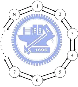
Figure 2.1 shows that the topology of the RPR network. The RPR ring network consists of two rings each using a unidirectional, counter-rotating ringlet. Nodes can transmit frames in clockwise direction by using one ringlet called the outer ring, and also transmit frames in counter clockwise direction by using the other ringlet called inner ring. This can be seen as two independent, symmetric counter rotating ringlets. The RPR protocol operates by sending data traffic in one direction and its corresponding control information in the opposite direction on the opposite ringlet. Each station receives the data frames from its upstream node; also it receives the control frames from the downstream node.
The RPR MAC provides three kinds of services, which are called Class A, Class B, and Class C services, to its upper layer. The Class A service is the service for the delivery of delay and jitter sensitive traffic. The Class B service is the service for the delivery of
bounded delay transfer of traffic at or below the committed information rate (CIR) and a best effort transfer of the excess information rate (EIR). The Class C service is the service for the delivery of the best effort traffic. In order to achieve the quality of service, the Class A and Class B-CIR traffic are transmitted by allocating the reserved bandwidth of the link. The Class B-CIR traffic and the Class C traffic are called the fairness eligible (FE) traffic and are transmitted to the downstream node opportunistically. In order to prevent the frame loss in transit because of the buffer overflow, the RPR nodes run a distributed traffic transmission control mechanism called the fairness control mechanism.
Figure 2.1: RPR network structure
Figure 2.2 shows the station structure of the RPR node. The traffic from the upstream node is put into two different queues, which are called the Primary Transit Queue (PTQ) and the Secondary Transit Queue (STQ). The PTQ is the queue used to buffer the Class A and Class B-CIR from the upstream node and it will be served firstly. The STQ is the queue to store the FE traffic from the upstream node, and it will be served lastly. The traffic from upper layer of local station is put into three different queues. The
Class A and Class B-CIR traffic are put into the Queue A, the Class B-EIR traffic is put into the Queue B, and the Class C traffic is put into the Queue C. The traffic in the Queue A will be served with the second priority, the traffic in the Queue B will be served with the third priority, and the traffic in the Queue C will be served lastly, which is the same as the STQ. In the RPR network, the total transmission rate of the Class A and the Class B-CIR traffic which are buffered in the Queue A and the PTQ is respectly called reservedRate.
Figure 2.2: The station structure of RPR node
The reservedRate is ensured the allocated bandwidth and service guarantees. The transmission rate of the FE traffic from the upper layer is called addRate. The addRate means the amount rate of the FE traffic which is permitted to add to the ringlet in the local station by the fairness control mechanism. The transmission rate of the FE traffic from the upstream node is called fwRate. The fwRate means the FE traffic added into the STQ of the local station from the upstream node. The LINK_RATE is defined as the total
transmission rate of the output link in the local station. The upperbound of the total output transmission rate of the FE traffic is called the unreservedRate. The value of the unreservedRate is the difference of the LINK_RATE and the value of the reservedRate. In order to implement the fairness, the fairRate is defined. The fairRate is determined by the fairness control mechanism and it will be sent to the upstream node to limit the addRate of the upstream node. When the local station received the fairRate from the downstream node, the received fairRate will be sent to the rate controller and the fairness control mechanism. Both of the aggressive mode and the conservative mode fairness control mechanism defined in the 802.17 specification limit the addRate and the STQ output rate by the fairRate. When the node receives the fairRate from the downstream node, it sends the received fairRate to the Rate Controller. If the node is congested, i.e. the STQ occupancy of the node exceeds the pre-determined threshold; it compares the received fairRate and the local fairRate which is calculated by the fairness control mechanism locally. The smaller fairRate will be sent to the upstream node.
In the fuzzy fairness control mechanism we proposed, the fairRate for the upstream node and the STQ output rate will be determined. Then the STQ output rate will be sent to the Rate Controller, and the new fairRate will be sent to the upstream node. The method to determine the fairRate and the STQ output rate will be described in section III. The Rate Controller is a hardware controller to control the transmission rate of the FE traffic. It controls the traffic from the Queue B and the Queue C according to the received fairRate, and controls the traffic from the STQ by the STQ output rate. Finally the output of the Rate Controller will be multiplexed with the traffic from the Queue A and the PTQ, and be transmitted to the downstream node.
2.2 Source Model
The three kinds of traffic, real-time voice, real-time multimedia, and none-real-time data, are considered in our work. Since the real-time voice traffic can’t torrent delay and jitter, it is classified as the Class A traffic. The real-time multimedia traffic permits bounded delay and jitter, so it is classified as the Class B traffic. The none-real-time data traffic is classified as the Class C traffic. In [10], we know that the traffic in a real network does not just arrive and leave according to Poisson process. The burstiness and the self-similarity should be considered. Here we will use the ON/OFF model to generate the constant bit rate (CBR) voice traffic that exhibit the properties of self-similarity, and the Sup-FRP Model will be used to generate the variable bit rate (VBR) multimedia and data traffic that exhibit the properties of self-similarity.
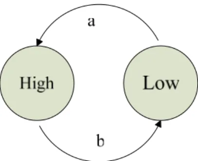
Figure 2.3: The ON/OFF model
Figure 2.3 shows the ON/OFF model which is characterized by a two-state discrete-time Markov train traffic model. It will generate Class-A packets during ON state but none during OFF state. The mean durations of ON and OFF periods are assumed to be exponentially distributed with 1/a and 1/b.
Figure 2.4: The bursty traffic model
The real-time multimedia traffic is divided as three kinds of frames, the Intra frame (I frame), the Predicted frame (P frame), and the Bidirectional frame (B frame). The I frame is the most important frame in a video because it contains the most image information in the three kinds of the frames. In this thesis we set I-frame as the Class-B CIR traffic and put it into the PTQ. The P frames and B frames will set as the Class-B EIR traffic and put into the STQ. The Class-B traffic and the Class-C traffic are generated by the bursty traffic model shown in Figure 2.4. The bursty traffic model is similar to the ON/OFF model. But the bursty traffic model will generate packet in both the high period and the low period. The packet inter-arrival time in the high period will be shorter than the packet inter-arrival time in the low period.
The traffic load of the bursty traffic model is controlled by the parameters of the arrival rate in the High state (RHigh), the arrival rate in the Low state (RLow), the change rate from the Low state to the High state (a), and the change rate from the High state to the Low state (b). The mean rate (λ) of the traffic load generated by the source can be obtained by b a aR bRhigh LOW + + = λ . (1)
Chapter 3
Fuzzy Fairness Control Mechanism
3.1 Fuzzy Inference System (FIS)
Fuzzy logic is based on the concepts of linguistic variables and fuzzy sets theory. A
fuzzy set in a universe of discourse U is characterized by a membership function μ(·)
which takes values in the interval [0, 1]. A fuzzy set F is represented as a set of ordered pairs, each made up of a generic element u∈U and its degree of membership μ(u). A
linguistic variable x in a universe of discourse U is characterized by T(x) =
{ } and M(x) = { }, where T(x) is the fuzzy term
set, i.e., the set of linguistic values’ names the linguistic variable x can take, and
is the membership function with respect to the term . If, for instance, x indicates the temperature, T(x) could be the set as {Low, Medium, High}, and each element in T(x) is associated with a membership function.
k x i x x T T T1,..., ,..., M1(u),...,M (u),...,Mk(u) x i x x i x T ) (u Mi x i x T
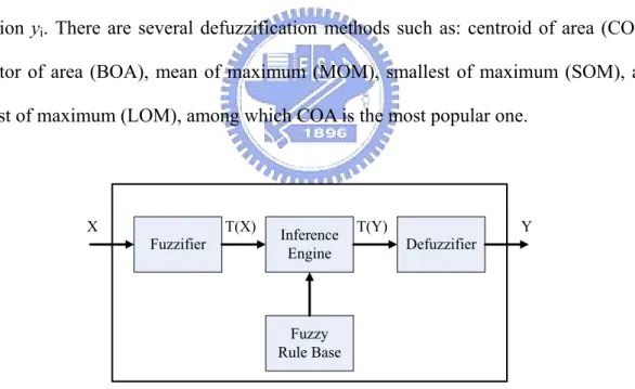
The fuzzy inference system (FIS) is a popular computing framework based on the concept of fuzzy logic and fuzzy reasoning. As shown in Figure 3.1, a fuzzy inference
system consists of four fundamental blocks: fuzzifer, fuzzy rule base, inference engine, and defuzzfier. The fuzzfier performs a mapping function from the observed value of each input linguistic variable xi to the fuzzy term set T(xi) with associated set of membership
degree M(xi), i = 1,…,m. The fuzzy rule base is a knowledge base characterized by a set
of linguistic statements in a form of “if-then” rules that describe a fuzzy logic relationship between the m-dim input linguistic variables {xi} and the n-dim output linguistic
variables {yi}. The inference engine performs an implication function according to the
pre-condition of the fuzzy rule with the input linguistic terms. It is a decision-making logic that acquires the input linguistic terms of T(yi). The defuzzifier adopts a
defuzzification function to convert T(yi) into a non-fuzzy value that represents the
decision yi. There are several defuzzification methods such as: centroid of area (COA),
bisector of area (BOA), mean of maximum (MOM), smallest of maximum (SOM), and largest of maximum (LOM), among which COA is the most popular one.
Fuzzifier InferenceEngine Defuzzifier
X T(X) T(Y) Y
Fuzzy Rule Base
Figure 3.1: The basic structure of the fuzzy inference system
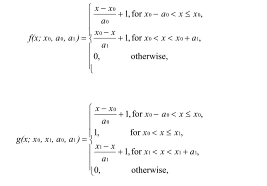
In this thesis, we use the triangular function f(x; x0, a0, a1) and the trapezoidal function g(x; x0, x1, a0, a1) to define the membership functions for terms in the term set. The two functions f(x; x0, a0, a1) and g(x; x0, x1, a0, a1) are given by
⎪ ⎪ ⎪ ⎩ ⎪ ⎪ ⎪ ⎨ ⎧ + < < + − ≤ < − + − = otherwise, , 0 , for , 1 , for , 1 1 0 0 1 0 0 0 0 0 0 1 0 0 x x x a a x x x x a x a x x ) , a , a f(x; x (2) and ⎪ ⎪ ⎪ ⎩ ⎪ ⎪ ⎪ ⎨ ⎧ + < < + − ≤ < ≤ < − + − = otherwise, , 0 , for , 1 , for , 1 , for , 1 1 1 1 1 1 1 0 0 0 0 0 0 1 0 1 0 a x x x a x x x x x x x a x a x x ) , a , a , x g(x; x (3)
where x0 in f(·) is the center of the triangular function; x0(x1)in g(·) is the left (right) edge of the trapezoidal function; and a0(a1) is the left (right) width of the triangular or the
trapezoidal function.
3.2 The Fuzzy Fairness Control Mechanism
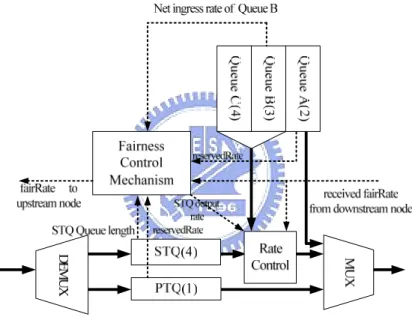
Figure 3.2 show that the fairness control mechanism, which generates the fairRate and the STQ output rate. In the RPR network, the fairRate and the STQ output rate are calculated and used in each unit time, where the duration is of unit time is 100μs and the length is an aging interval defined in the 802.17 specification. The fairRate and the STQ output rate will be computed and sent at the end of a unit time, but the other parameters will be measured or received by the fairness control mechanism at the beginning of a unit time. There are two important factors to determine the fairRate to the upstream node. One is the STQ status, and the other is the output transmission rate of the node. Since STQ is used to buffer the FE traffic, if the STQ is in a high occupancy, the
fairRate should be decreased to avoid frames losing. The output transmission rate is the available service rate of the local station due to the received fairRate. If the amount of the incoming traffic exceeds the output transmission rate, some traffic will be buffered in the queue system of the local station due to their low priority and causes the congestion because the RPR network does not drop any frame. For the above reasons, we use the Fuzzy Congestion Indication to indicate the STQ status in each unit time, and the Fuzzy STQ Output Rate Calculation to calculate the STQ output rate which is used in the next time unit. Finally, the new fairRate will be calculated by the Fuzzy fairRate Calculation according to the output of the Fuzzy Congestion Indication and the Fuzzy STQ Output Rate Calculation.
Figure 3.2: The fuzzy fairness control mechanism
3.2.1 Fuzzy fairRate Calculation (FfC)
The fairness control mechanism determines the fairRate for the upstream node according to two issues, the congestion and the available service rate. The congestion of the local station means that remain queue length of the STQ is not enough to buffer the transit traffic from the upstream node. In this situation, the value of the fairRate for the
upstream node is used to reduce the fwRate of the local station. We use the congestion degree, denoted by Dc(n), to indicate the occupancy and the variation of the STQ and represent the possibility of the congestion in the n-th unit time. The available service rate represents the capability of the local station to deal with the transit traffic from the upstream node. Since the congestion degree is determined by the STQ, we use the STQ output rate of the local station, denoted by os(n), in the n-th unit time to represent the available service rate. We can determine whether the fairRate should be decremented or not to prevent probably congestion in the local station according to this parameter. The STQ output rate is the service rate of the STQ in the n-th unit time so we can predict the amount of the transit traffic which is allowed to buffer in the STQ in the next time unit. The term set for the congestion degree is defined as T(Dc(n)) = {Very High (VH), High (H), Low (L), Very Low (VL)}; that for the STQ output rate is defined as T(os(n)) = {Very High (VH), High (H), Low (L), Very Low (VL)}; that for the determined fairRate is defined as T(r(n)) = {Extreme High (EH), Very High (VH), High (H), Low (L), Very Low (VL), Extreme Low (EL)}.
The membership functions for VH, H, L, and VL in T(Dc(n)) are denoted by
μVH(Dc(n)), μH(Dc(n)), μL(Dc(n)), and μVL(Dc(n)) and they are defined for
μVH(Dc(n))= f(Dc(n); 1, 0.25, 0) (4)
μH(Dc(n))= f(Dc(n); 0.75, 0.3, 0.25) (5)
μL(Dc(n))= f(Dc(n); 0.45, 0.25, 0.3) (6)
μVL(Dc(n))= f(Dc(n); 0, 0, 0.45) (7)
The membership functions for VH, H, L, and VL in T(os(n)) are denoted by μVH(os(n)), μH(os(n)), μL(os(n)), and μVL(os(n)), and they are defined as μVH(os(n))= g(os(n); 0.8RL, RL, 0.2RL, 0) (8)
μH(os(n))= f(os(n); 0.6RL, 0.2RL, 0.2RL) (9)
μL(os(n))= f(os(n); 0.4RL, 0.2RL, 0.2RL) (10)
μVL(os(n))= g(os(n); 0, 0.2RL, 0, 0.2RL) (11)
where RL is the link rate of the output link. The fuzzy inference algorithm is min-max inference method. The defuzzification method we used is the center of area defuzzification method. The membership function for EL, VL, L, H, VH, and EH in r(n) are denoted by μEL(r(n)), μVL(r(n)), μL(r(n)), μH(r(n)), μVH(r(n)), μEH(r(n)), and they are defined as μEL(r(n))= f(r(n); 0, 0, 0) (12) μVL(r(n))= f(r(n); 0.2 RU, 0, 0) (13) μL(r(n))= f(r(n); 0.4 RU, 0, 0) (14) μH(r(n))= f(r(n); 0.4 RU, 0, 0) (15) μVH(r(n))= f(r(n); 0.8 RU, 0, 0) (16) μEH(r(n))= f(r(n); RU, 0, 0) (17) where RU is the unreserved rate of the output link.
The fuzzy rules of the fairRate calculation are shown in Table 3.1. We do not only determine the fairRate based on the congestion degree, but the STQ output rate is also considered. If the STQ output rate is high or very high, the fairRate will not be very low or extreme low even if the congestion degree is very high because that the congestion degree will level down for the high STQ output rate.
Table 3.1
The rule base of the fairRate calculation
Rule Dc(n) os(n) r(n) Rule Dc(n) os(n) r(n) 1 VH VL EL 9 L VL L 2 VH L VL 10 L L H 3 VH H L 11 L H VH 4 VH VH L 12 L VH VH 5 H VL VL 13 VL VL H 6 H L VL 14 VL L H 7 H H L 15 VL H VH 8 H VH H 16 VL VH EH
3.2.2 Fuzzy Congestion Indication (FCI)
The FCI is used to determine the congestion degree in the time unit. In the RPR network, the queue length of the STQ can present the amount of the buffered transit FE traffic. If the queue length is long, the local station may in a congested condition. Also, if the queue length of the STQ is still getting longer, the congestion of the local station may be more serious. Therefore, we measure the net input rate of the STQ in the previous unit time, denoted by Ns(n-1), and the STQ length at the beginning of the n-th unit time, denoted by Ls(n), to indicate the congestion degree of the local station in the n-th unit time, Dc(n). The term set for the net input rate of the STQ is defined as T(Ns(n-1)) = {Increment Large (IL), Increment Small (IS), Decrement Small (DS), Decrement Large (DL)}; for the STQ length is defined as T(LS(n)) = {Long (L), Medium (M), Short (S)}; for the congestion degree is defined as T(Dc(n)) = {Very high, High, Low, Very low}.
The membership functions for IL, IS, DL, and DS in T(Ns(n-1)) are denoted by
μIL(Ns(n-1)), μIS(Ns(n-1)), μDS(Ns(n-1)), and μDL:(Ns(n-1)), and they are
μIS(Ns(n-1))= f(Ns(n-1); 0.25Q, 0.25Q, 0.25Q) (19)
μDS(Ns(n-1))= f(Ns(n-1); −0.25Q, 0.25Q, 0.25Q) (20)
μDL(Ns(n-1))= g(Ns(n-1); −Q, −0.5Q, 0, 0.25Q) (21)
Note that we measure the net input rate as a ratio with STQ size in a unit time. The membership functions for L, M, and S in T(LS(n)) are denoted by μL(LS(n)), μM(LS(n)), and μS(LS(n)), and they are μL(LS(n))= f(LS(n); Q, 0.25Q, 0) (22)
μM(LS(n))= f(LS(n); 0.75Q, 0.25Q, 0.125Q) (23)
μS(LS(n))= g(LS(n); 0, 0.5Q, 0, 0.25Q), (24)
where Qis the size of the STQ. The fuzzy inference algorithm is also min-max inference method. The defuzzification method we used is the center of area defuzzification method. The membership function for VL, L, H, and VH in Dc(n) are denoted by μVL(Dc(n)), μL(Dc(n)), μH(Dc(n)), μVH(Dc(n)), and they are defined as μVL(Dc(n))= f(Dc(n); 0.2, 0, 0) (25)
μL(Dc(n))= f(Dc(n); 0.4, 0, 0) (26)
μH(Dc(n))= f(Dc(n); 0.6, 0, 0) (27)
μVH(Dc(n))= f(Dc(n); 0.8, 0, 0) (28) The fuzzy rules of the fairRate calculation are shown in Table 3.2. We determine the level of the congestion degree according to the length of the STQ as the original fairness control mechanism. The net input rate is the reference to modify the congestion degree. If the net input rate is decrement largely, the congestion degree will be leveled down. Oppositely, the congestion degree will be leveled up by the highly increment of the
net input rate.
Table 3.2
The rule base of the fuzzy congestion indication
Rule Ns(n-1) LS(n) Dc(n) Rule Ns(n-1) LS(n) Dc(n) 1 IL L VH 7 DL M L 2 IS L VH 8 DS M L 3 DL L H 9 IL S H 4 DS L VH 10 IS S L 5 IL M H 11 DL S VL 6 IS M H 12 DS S VL
The FCI is used to estimate the congestion condition of the local station. In the original fairness control mechanism, if the STQ occupancy is higher than the pre-determined threshold, the fairness mechanism will start to throttle the transmission rate of the upstream nodes. But sometimes the STQ occupancy can’t represent if the congestion will happen or but. Therefore, we set the default threshold as the boundary of the membership function in FCI instead of letting the threshold be fixed. Also we consider the net input rate of the STQ to show the variation of the STQ. The STQ occupancy shows that the buffer usage of the local node and the net input rate of the STQ show that the STQ usage is getting higher or lower. If the usage is getting lower, we can give a larger value of the fairRate to the upstream node because of the more space of the STQ will be release in the next unit time. So the FCI can predict the congestion degree more exactly.
3.2.3 Fuzzy STQ Output Rate Calculation (FSORC)
The STQ output rate is an important factor to determine the fairRate. It limits the amount of the transit traffic in the STQ which can be passed to the downstream node in the unit time. In the original fairness control mechanism, the STQ output rate is limited by the fairRate, too. However, if the node has not much local ingress traffic, the STQ output rate should be given a high rate to accelerate the decreasing of the STQ occupancy. Therefore, in the fuzzy fairness control mechanism, we define the method to estimate the appropriate STQ output rate.
There are two important factors to determine the STQ output rate. One is the difference of the received fairRate, denoted by drf(n), which shows that the variation of the received fairRate from the downstream node. The received fairRate can represent the capacity of the STQ in the downstream node. According to the received fairRate, the addRate of the local station will be limited. The total output transmission rate will be determined. The STQ output rate is influences the total output transmission rate. If the received fairRate increases, the total output transmission rate may increase and the STQ output rate may increase. On the contrary, if the received fairRate decreases, the total transmission rate will decrease and the STQ output rate will decrease. The other factor is the ingress traffic of the local station in the previous time unit, denoted by T(n-1), which has higher priority than the traffic in the STQ. Since the STQ is served lastly, the ingress traffic of the PTQ, Queue A, and Queue B should be served before the STQ. The amount of the traffic in PTQ, Queue A, and Queue B will directly influence the STQ output rate due to their priority. The term set for the difference of the received fairRate is defined as
T(drf(n)) = {Positive High (PH), Positive Low (PL), Negative High (NH), Negative Low
STQ is defined as T(T(n-1)) = {Big (B), Small (S)}; for the determined STQ output rate is defined as T(os(n)) = {Very High (VH), High (H), Low (L), Very Low (VL)}.
The membership functions for PH, PL, NL, and NH in T(drf(n)) are denoted by
μPH(drf(n)), μPL(drf(n)), μNL(drf(n)), and μNH(drf(n)), and they are
μPH(drf(n))= f(drf(n); RL, 0.75RL, 0) (29)
μPL(drf(n))= f(drf(n); 0.25RL, 0.25RL, 0.25RL) (30)
μNL(drf(n))= f(drf(n); −0.25RL, 0.25RL, 0.25RL) (31)
μNH(drf(n))= f(drf(n); −RL, 0, 0.75RL) (32)
where RL is the link rate of the output link. The membership functions for B and S in T(T(n-1)) are denoted by μB(T(n-1)), and μS(T(n-1)), and they are μB(T(n-1))= g(T(n-1); 0.6RL, RL, 0.4RL, 0.4RL) (33)
μS(T(n-1))= f(T(n-1); 0, 0, 0.4RL) (34)
where RL is the link rate of the output link. The fuzzy inference algorithm is also min-max inference method. The defuzzification method we used is the center of area defuzzification method. The membership function for VL, L, H, and VH in os(n) are denoted by μVL(os(n)), μL(os(n)), μH(os(n)), μVH(os(n)), and they are defined as μVL(os(n))= f(os(n); 0.2 RU, 0, 0) (35)
μL(os(n))= f(os(n); 0.4 RU, 0, 0) (36)
μH(os(n))= f(os(n); 0.6 RU, 0, 0) (37)
where RU is the unreserved rate of the output link.
The fuzzy rules of the fairRate calculation are shown in Table 3.3. We determine the STQ output rate based on the deference of the received fairRate. If the received fairRate increases, the corresponding STQ output rate will be set in a high level. Oppositely if the received fairRate decreases, the STQ output rate will be set in a low level. The ingress traffic in the previous time unit which has higher priority than the STQ is a reference value to adjust the STQ output rate. The STQ output rate will be leveled down because of the large amount of the ingress traffic with high priority.
Table 3.3
The rule base of the STQ output rate calculation
Rule drf(n) T(n-1) os(n) Rule drf(n) T(n-1) os(n)
1 PH S VH 5 NL S H 2 PH B H 6 NL B L 3 PL S H 7 NH S L 4 PL B L 8 NH B VL
Chapter 4
Simulation Results and Discussions
4.1 Simulation Environment
In this section, a time-driven packet-based simulation is developed to show the performance of the proposed fuzzy fairness control mechanism (FFCM) presented in the previous chapter. We consider the RPR architecture with five nodes. The link bandwidth between the stations is considered to be 1Gbps. The propagation delay is set to 0.2ms. The aggressive mode (AM) fairness control mechanism is implement to compare with the FFCM.
Three kinds of traffic are considered in the system: voice, video, and data. The voice traffic is transmitted as the Class A traffic with the highest priority, and is generated by an ON/OFF model defined in Chapter 2. The video traffic is transmitted as the Class B traffic. The main frames of the video will be transmitted as the Class B-CIR traffic, the others will be sent as the Class B-EIR. The data traffic will be transmitted as the Class C
traffic.
Figure 4.1 shows the simulation model. There are five nodes in the RPR ring which is indicated by node 1, node 2, node 3, node 4, and node 5. The corresponding link to transmit the data frames from node 1, node2, node3, and node 4 is called link 1, link 2, link 3, and link4. In this simulation model, we define four flows which indicate the ingress traffic to node 5. The flow 1, for instance, means the traffic from node 1 to node 5 which is transit in node 2, node 3, and node 4. The flow 2, flow 3, and flow 4 is similar to the flow 1.
Figure 4.1: The simulation model
Each flow consists of the fairness eligible traffic, i.e. the Class B-EIR traffic and the Class C traffic, with a mean traffic rate. The mean traffic rate is a ratio of the link capacity. If the rate is 0.1, for instance, the traffic load is 100Mbps. The Class B-EIR traffic and the Class C traffic will be generated by the bursty traffic model with the arrival rate of the High state is set to 0.9 and the arrival rate of the Low state is set to 0.1. We can adjust the change probability to generate different traffic load. The Class A and the Class B-EIR traffic will be generated be the ON/OFF model and the Sup-FRP Model. The total traffic load of the Class A and the Class B-EIR will vary in the range of 10Mpbs to
100Mbps.
There are two scenarios in our simulation, the balance mode and the unbalance mode. In the balance mode, all the flows have the same traffic load. As the traffic load of each flow is getting higher, the link 4 will be overloaded, and the node 4 will become congested. We observe the link utilization of the link 2 and link 3 to show that the fuzzy fairness control mechanism is able to control the congestion as the aggressive mode fairness control mechanism which is defined by the 802.17 standard. In the unbalance mode, the traffic load of the flow 2 and the flow 4 is fixed at 0.1, and we change the traffic load of the flow 1 and flow 3 from 0.15 to 0.4. As in the balance mode, the node 4 will become congested, too, but the fair rate will over throttle the transit traffic from the upstream node of node 4 because of the extreme low load of the node 4. In the unbalance mode, we will observe the link utilization and the access delay of each flow to test and verify the influence of the over throttle behavior; also we will show that the fuzzy fairness control mechanism can improve the performance.
4.2 Simulation Results
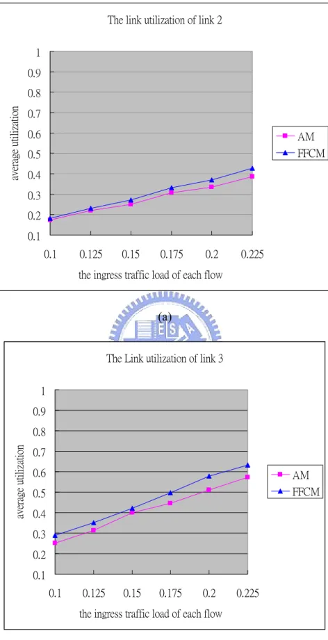
Figure 4.2 shows the link utilization of the link 2 and link 3 in the balance mode. The ingress traffic load is set from 0.1 to 0.225, i.e. the system traffic load is set from 0.4 to 0.9. In Figure 4.2 (a), we can observe that the performance of the aggressive mode and the fuzzy fairness control mechanism are nearly the same. This result shows that when the system load is light and balance, both of the two fairness control mechanism work well because the node does not become congested frequently. But in Figure 4.2(b), when the load is getting higher, the utilization of the link 3 under aggressive mode is clearly lower than the utilization under the fuzzy fairness control mechanism. The reason of this
result is that the node 4 is treated as congested only when the STQ occupancy exceeds the pre-determined threshold in the aggressive mode, but the node information, such as the net input rate of the STQ and the STQ output rate of the local node, is considered to determine whether the node is congested or not in fuzzy fairness control mechanism. Even if the STQ occupancy is in a really high position, the FFCM may not treat the node as congestion because of the low net input of the STQ and the high STQ output rate. In other words, the frequency of the congestion in fuzzy fairness control mechanism is less than in the aggressive mode.
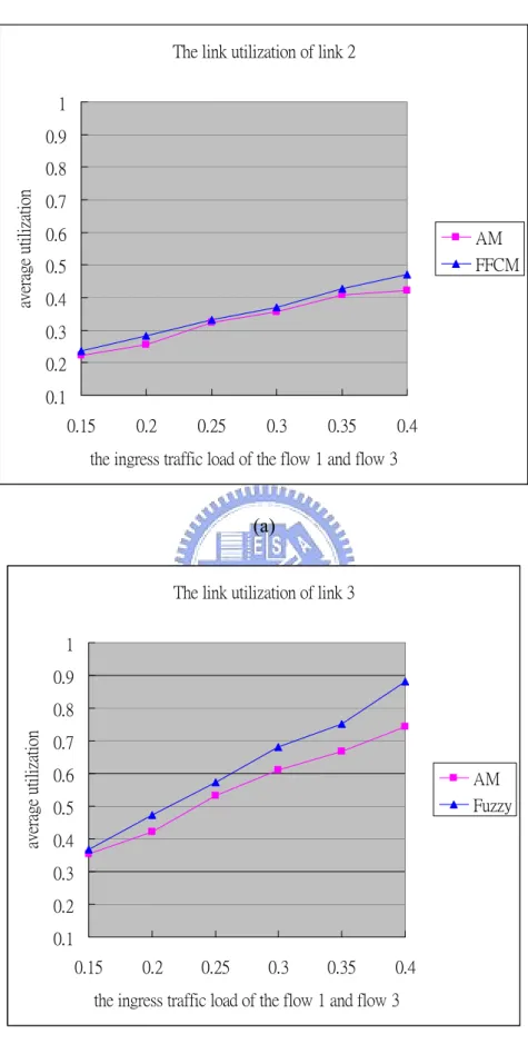
In Figure 4.3, the utilization of the link 2 and link 3 is shown. The horizontal axis is the ingress traffic load of the flow 1 and flow 3 in the unbalance mode. Both of the ingress traffic loads of flow 2 and flow 4 are set at 0.1. In Figure 4.3(a) the utilization is similar as Figure 4.2(a) because of the low traffic load which transit by the link 2, but in Figure 4.3(b) we can observe that the utilization of the link 3 under the fuzzy fairness control mechanism is deferent obviously because of the over throttle problem.
When the node 4 is congested, it will send it’s addRate as fairRate to the upstream node firstly. In the unbalance mode, the addRate of the node 4 is less than 0.1 because of the low ingress traffic load, so the unreasonable fairRate is sent to the node 3. This fairRate causes that the ingress traffic of the node 3 is limited excessively. The utilization of link 3 decreases clearly because of the unnecessarily limitation. In our fuzzy fairness control mechanism, as the occupancy of the STQ in node 4 is getting higher, the node 4 will send a lower fairRate to its upstream node, too. To differ with the aggressive mode, the ingress traffic load and the STQ output rate is considered, and node 4 will determine a higher fairRate because of the lower local ingress traffic load and the higher STQ output rate. This behavior can estimate the appropriate fairRate more correctly and prevent the
The link utilization of link 2 0.1 0.2 0.3 0.4 0.5 0.6 0.7 0.8 0.9 1 0.1 0.125 0.15 0.175 0.2 0.225 the ingress traffic load of each flow
ave rage ut ili zat io n AM FFCM (a)
The Link utilization of link 3
0.1 0.2 0.3 0.4 0.5 0.6 0.7 0.8 0.9 1 0.1 0.125 0.15 0.175 0.2 0.225
the ingress traffic load of each flow
av erag e u tili za ti on AM FFCM (b)
over-throttle problem to decrease the utilization.
For the reason we described in the previous paragraph, the ingress traffic of node 3 will be limited excessively. In Figure 4.4(a), we can observe that by the access delay performance of each flow, and we notice that the access delay of the flow 1 is distinct unreasonable higher in the aggressive mode. When the congestion happens, the fairRate which is sent to all nodes in the congestion domain is the same. So the flow 1 is over throttled as the flow 3 because of the high ingress traffic load which is the same as the flow 3.
In Figure 4.4(b), we can find that the access delay of each flow is almost the same. The fuzzy fairness control mechanism does not only prevent the over-throttle problem but also allocates the link capacity for all the ingress traffic flow more efficiently. The node with heavy traffic load will be allocated more link bandwidth to transmit the ingress traffic before the delay bound. As the result shows in Figure 4.4(b), the access delay is fairly distributed between all flows. In the aggressive mode, the access delay of the flow 1 and flow 3 are higher than the flow 2 and flow 4 because of the fairness access probability of each flow which is controlled by the fairness control mechanism. This problem is improved by FFCM because the link bandwidth is shared according to the traffic load of the flows.
The link utilization of link 2 0.1 0.2 0.3 0.4 0.5 0.6 0.7 0.8 0.9 1 0.15 0.2 0.25 0.3 0.35 0.4
the ingress traffic load of the flow 1 and flow 3
ave rage uti lizat ion AM FFCM (a)
The link utilization of link 3
0.1 0.2 0.3 0.4 0.5 0.6 0.7 0.8 0.9 1 0.15 0.2 0.25 0.3 0.35 0.4
the ingress traffic load of the flow 1 and flow 3
av erag e u tili za ti on AM Fuzzy (b)
average access delay of AM 0 50 100 150 200 250 300 350 400 450 500 0.15 0.2 0.25 0.3 0.35 0.4 the ingress traffic load of flow 1 and flow 3
acc ess del ay( m s) flow1 flow2 flow3 flow4 (a)
average access delay of FFCM
0 50 100 150 200 250 300 350 400 450 500 0.15 0.2 0.25 0.3 0.35 0.4 the ingress traffic load of flow 1 and flow 3
access del ay(m s) flow1 flow2 flow3 flow4 (b)
Figure 4.4: The access delay of each flow in the unbalance mode (a) aggressive mode (b) the fuzzy fairness control mechanism.
Chapter 5
Conclusion
In this thesis, we propose a fuzzy fairness control mechanism to solve the problems which exist in the aggressive mode fairness control mechanism. The goal is to increase the link utilization and to share the link capacity to each node effectively. We study the architecture of node and network architecture in RPR which is defined in standard 802.17. The proposed fuzzy fairness control mechanism is divided as three parts. First, we decide the congestion degree of the node by observing the STQ input rate and STQ occupancy. Second, we calculate the STQ output rate by gathering the fairRate from the downstream node and the ingress traffic load information. Finally, we determine the fairRate to the upstream node to limit the traffic to the node.
The proposed fuzzy fairness control mechanism is compared to the aggressive mode fairness control mechanism. To differ with the aggressive mode, the congestion does not be determined to happen only when the STQ occupancy exceeds the pre-defined threshold, and we calculate the fairRate with more information of the node instead of setting the addRate as the fairRate firstly. As the result of that, the STQ can be utilized
effectively, and the fairRate is estimated more reasonably.
Simulation results show that the utilization of the link in the mechanism we proposed is higher than in the aggressive mode because the over-throttle problem is prevented and the congestion does not happen excessively persistently. Also the access delay of each node will become almost the same even if the ingress traffic load of each node is different. The fairness to access the RPR ring of all the nodes is improved. The fuzzy fairness control mechanism is more feasible and robust for the RPR network then aggressive mode fairness control mechanism.
Bibliography
[1] T. H. Wu and W. Way, “A novel passive protected SONET bi-directional self-healing ring architecture,” MILCOM’91, Conference Record, 'Military Communications in a Changing World',
IEEE, vol.3, pp.894-900, Nov. 1991.
[2] IEEE Standard 802.17, Resilient Packet Ring (RPR) access method and physical layer specification, Sept. 2004
[3] F. Davik, M. Yilmaz, S. Gjessing, and N. Uzun, “IEEE 802.17 resilient packet ring tutorial,” IEEE
Communication Magazine, vol.42, no.3, pp.112-118, March 2004.
[4] F. Davik and S. Gjessing, “The Stability of the resilient packet ring aggressive fairness algorithm,” in Proceedings of the 13th IEEE Workshop on Local and Metropolitan Area Network
(LANMAN2004), April, 2004, pp. 17-22.
[5] F. Davik, A. Kvalbein, and S. Gjessing, “An analytical bound for convergence of the resilient packet ring aggressive mode fairness algorithm,” in Proceedings of the IEEE ICC May, 2005. [6] F. Davik, A. Kvalbein, S. Gjessing, and N. Uzun, “Improvement of resilient packet ring fairness,”
in Proceedings of the Global Telecommunications Conference, 2005, Volume 1, Nov, 2005. [7] Y. F. Robichaud and C. C. Huang, “Improvement fairness algorithm to prevent tail node induced
oscillations in RPR,” in Proceedings of the IEEE ICC May, 2005.
[8] T.J.Kim, “An enhanced fairness algorithm for the IEEE 802.17 resilient packet ring,” IEICE
Transactions of Communication, May, 2005.
[9] D.H. Lee, and J.H. Lee, “A novel fairness mechanism based on the number of effective nodes for efficient bandwidth allocation in the resilient packet ring, ”IEICE Transactions of
[10] W.E. Leland, M.S. Taqqu, W. Willinger, and D. V. Wilson, “On the self-similar nature of ethernet traffic (extended version), ”IEEE/ACM Transactions on networking, vol.2, no.1, Feb,