以多項式消除編碼為基礎之OFDM系統頻率估計

國

立

交

通

大

學

電機學院通訊與網路科技產業研發碩士班

碩

士

論

文

以多項式消除編碼為基礎之 OFDM 系統頻率估計

CFO Estimation for Polynomial Cancellation Coded OFDM Systems

研 究 生：洪千雅

指導教授：蘇育德 教授

以多項式消除編碼為基礎之 OFDM 系統頻率估計

CFO Estimation for Polynomial Cancellation Coded OFDM Systems

研 究 生：洪千雅 Student：Chien-Ya Hung

指導教授：蘇育德 Advisor：Y.T. Su

國 立 交 通 大 學

電機學院通訊與網路科技產業研發碩士班

碩 士 論 文

A Thesis

Submitted to College of Electrical and Computer Engineering National Chiao Tung University

in partial Fulfillment of the Requirements for the Degree of

Master in

Industrial Technology R & D Master Program on Communication Engineering

August 2008

Hsinchu, Taiwan, Republic of China

i 1

以多項式消除編碼為基礎之 OFDM 系統頻率估計

學生：洪千雅

指導教授

：

蘇育德

國立交通大學電機學院產業研發碩士班

摘

要

正交多頻分工(Orthogonal Frequency Division Multiplexing ,OFDM)技

術近年來頗受到重視。OFDM 系統設計必需要考慮到載波頻率偏移(CFO)補償這

個課題，因為載波頻率偏移會造成載波彼此之間的與干擾(ICI)，破壞載波的

正交性並將大大的降低系統效能。載波彼此之間的干擾(ICI)會使載波上的信

號強度衰減(attenuation)並產生相角旋轉 (phase rotation)。在許多消除

ICI 的方法中，ICI 自我消除法(ICI self-cancellation) 或稱為多項式消除

編碼(polynomial cancellation coding, PCC)因其容易實現以及效能穩定而

受到重視。然而，當載波頻率偏移大時，多項式消除編碼只能消除一小部份

的 ICI。因此，我們提出以多項式消除編碼為基礎的載波頻率偏移估計。首先，

以 PCC 做為事前編碼 (precoding)並解出初步的資料，接下來再以此資料估

計載波頻率偏移(CFO)。藉由使用多項式消除編碼，直接估出載波頻率偏移

(CFO)並加以補償，可以改善原本多項式消除編碼在載波頻率偏移(CFO)大時

只能消除部份 ICI 的缺失。

CFO Estimation for Polynomial Cancellation Coded OFDM Systems

student：Chien-Ya Hung

Advisors：Dr.

Y.T. Su

Industrial Technology R & D Master Program of

Electrical and Computer Engineering College

National Chiao Tung University

ABSTRACT

Orthogonal Frequency Division Multiplexing (OFDM) is being considered as a promising

transmission technique. However, a carrier frequency offset (CFO) between the transmitter

and receiver will results in ICI and thus destroy the orthogonality of the subcarrier and

degrades the performance. ICI leads to attenuation and phase rotation of desired signal on

each subcarrier. These impairments have already motivated several studies to find solutions.

Among the several ICI reduction schemes, ICI self-cancellation or polynomial cancellation

coding (PCC) scheme has received much attention due to its simplicity and its high robustness

to frequency offset errors. However, for large CFO, PCC can only eliminate ICI to a certain

extent. Thus, we propose new methods of PCC based CFO estimation to eliminate ICI for

either low or high CFOs. First, we use PCC as precoding scheme and get the initial decoded

data. Then CFO estimation is done by making use of the decode data. CFO estimation and

compensation from PCC can overcome the drawback of PCC that only a certain part of ICI

can be eliminated when CFO is large.

iii

誌

謝

本論文得以順利完成，首先要感謝我的指導老師蘇育德教授，在

我研究所的生涯中，不厭其煩地賜予方向與教導。也謝謝蒞臨的口試

委員們所提出的建議，使本論文得以更加完整。更感謝實驗室每一位

優秀、熱心的學長姐與可愛的學弟妹們，你們總是在我最需要的時

候，不吝伸出援手。

更感謝一直陪伴在我身邊的摯友，以及最關心我的家人們。

Contents

English Abstract

i

Chinese Abstract

ii

Contents

iv

List of Figures

vi

1 Introduction

1

2 Polynomial Cancellation Coded OFDM Systems

3

2.1

Introduction………

3

2.2 System Model………. 4

2.3

Polynomial

Cancellation Coding………... 4

2.3.1 Overview………

4

2.3.2 ASR………

6

2.3.3 SSR……….

9

3 CFO Estimation for ASR of Polynomial Cancellation Coding

13

3.1 Modulation Scheme over AWGN Channel……… 13

3.2 Modulation Scheme over Fading Channel……….

17

3.3 Demodulation Scheme over AWGN Channel………

18

3.4 Demodulation Scheme over Fading Channel……….

21

4 CFO Estimation for SSR of Polynomial Cancellation Coding

22

4.1 Modulation Scheme over AWGN Channel……… 26

v

4.2 Modulation Scheme over Fading Channel………. 27

4.3 Demodulation Scheme over AWGN Channel……… 29

4.4 Demodulation Scheme over Fading Channel………. 30

5 Simulation Results and Discussions

33

6 Conclusion

34

vi

List of Figures

1. A typical OFDM modulator……… 3

2. A typical OFDM demodulator……… 3

3. An example of s l( − for = 16  = 0 Real part ofk) 　 　　 　 s l( − ……….k) 5 4. An example of s l( − for = 16  = 0 Real part ofk) 　 　　 　 s l( − ……….k) 5 5. A comparison between s l( − ,k) s l'( −k)and s l"( −k)……….. 7

6. BER of ASR demodulation scheme over AWGN channel……….. 8

7. BER of ASR demodulation scheme over fading channel……… 9

8. BER of SSR demodulation scheme over AWGN channel……….. 10

9. BER of SSR demodulation scheme over fading channel………. 11

10. Re{ ( )Λ

ε

}with Λ( ) S

ε

= ₀− of ASR modulation scheme S₁ whenε is fom 0 to 1……… 16

11. Im{ ( )Λ

ε

}with Λ( ) S

ε

= ₀− of ASR modulation scheme S₁ whenε is from 0 to 1……… 17

12. Re{ ( )Λ

ε

}with Λ( ) 2S

ε

= ₀− −S₁ S₋₁ of ASR demodulation scheme whenε is from 0 to 1………. 22

13. Im{ ( )Λ

ε

}with Λ( ) 2S

ε

= ₀− −S₁ S₋₁ of ASR demodulation scheme whenε is from 0 to 1………... 23

14. Re{ ( )Λ

ε

}with Λ( )

ε

=S₀−S_N−1 of SSR modulation scheme whenε is from 0 to 1……… 27

15. Im{ ( )Λ

ε

}with Λ( )

ε

=S₀−S_N−1 of SSR modulation scheme whenε is from 0 to 1……… 28

16. Re{ ( )Λ

ε

}with Λ( ) 2

ε

= S₀−S_N−1−S_−(N−1) of SSR demodulation whenε is from 0 to 1……… 30

17. Im{ ( )Λ

ε

}with Λ( ) 2

ε

= S₀−S_N−1−S_−(N−1) of SSR demodulation whenε is from 0 to 1……… 31

18. Comparison of MSE of CFO with SNR=3dB over AWGN channel…………. 33

1

Introduction

Orthogonal Frequency Division Multiplexing (OFDM) is being considered as a promising transmission technique for high data rate wireless communication systems because of its su¢ -cient robustness to handle radio channel impairments and its bandwidth e¢ ciency [1]. Despite its bene…ts, one of its impairments is intercarrier interference (ICI) and is considered as one limiting factor for e¢ cient implementationof OFDM systems. An OFDM system uses a set of orthogonal subcarriers. This orthogonality allows the receiver to separate the data symbol on each subcarriers, which are overlapped at the transmitter to achieve spectral e¢ ciency. The loss of orthogonality results in ICI. This ICI deteriorates the bit error rate of the system and introduces an error ‡oor. This error ‡oor cannot be removed by just increasing the transmit power. Generally, the cause for ICI can be grouped into following categories: (i) carrier fre-quency o¤set errors, (ii) phase noise, (iii) IQ mismatch at the receiver front end and (iv) time selectivity of the wireless channel.

The characteristics of the above causes and the degree of their e¤ects are di¤erent. The …rst three causes are due to hardware imperfections and the later is due to unpredictable nature of wireless channel. Carrier frequency o¤set errors are caused by the mismatch of oscillators’frequencies between the transmitter and the receiver [2] where as phase noise is due to instability of an oscillator [2], [3]. Besides, the doppler frequency will also result in CFO. IQ mismatch refers to phase and gain imbalance between in-phase (I) and quadrature (Q) paths at the receiver front end [4], [5]. On the other hand, the fading channels generally exhibit both frequency selectivity and time selectivity. OFDM has been proposed to combat the frequency selectivity, but its performance might be a¤ected by the time selectivity. The resulting time selective fading causes a loss of subcarrier orthogonality, thus resulting in ICI [6]. These ICI causes also lead to attenuation and phase rotation of desired signal on each subcarrier. These impairments have already motivated several studies to …nd solutions. Among the several ICI reduction schemes, ICI self-cancellation [7] or polynomial cancellation coding (PCC) scheme has received much attention due to its simplicity and its high robustness to frequency o¤set

errors. In this technique, each data symbol is transmitted on two adjacent subcarriers with opposite polarity in order to cancel ICI. The data throughput of this scheme will therefore be half of that of conventional OFDM. Thus, this cancellation scheme is also referred to as rate-half repetition coding. This cancellation scheme is further extended to reduce more ICI by mapping data symbols onto a larger group of adjacent subcarriers [7], [8]. However, this further reduces the data throughput, despite more ICI reductions. In [9], rate 2/3 and 3/4 coding schemes has been proposed t o improve the data throughput with moderate ICI reduction. Authors in [l0] improved this cancellation scheme by transmitting the data symbols on k-th and (N-1-k)-th subcarriers, instead of adjacent subcarriers. This approach o¤ers a frequency diversity because of the frequency separation between the same data symbols. In this paper, we will refer adjacent ICI self-cancellation scheme [7], [8] as "Adjacent Symbol Repetition (ASR)" and the non-adjacent ICI self-cancellation scheme [10] as "Symmetric Symbol Repetition (SSR)".

However, ICI self-cancellation schemes have been veri…ed being e¤ective at low frequency o¤sets. For high frequency o¤sets, the ICI self-cancellation can only eliminate ICI components to a certain extent. The remaining frequency errors still degrade the system signi…cantly. The existing compensation methods based on the ICI self-cancellation for frequency o¤sets require either pilot information or training sequences [10]–[12]. Blind estimation methods are either only e¤ective for small frequency o¤sets or with considerable computational complexity [13]–[17]. Therefore, a simple acquisition and tracking approaches for compensating carrier frequency o¤set prior to the ICI self-canceling demodulation is developed [18], and CFO is estimated and compensated in the range from 0 to 0.5.

So far as to CFO estimation, there have been a multitude of proposals for CFO compensa-tion. A maximum likely hood estimate was proposed by Moose [19], based on the observation of two consecutive and identical symbols. Its maximum frequency acquisition range is 1=2 subcarrier spacing because of mod 2 ambiguity.

Here we propose new methods to estimate CFO by making use of the decoded data symbol from polynomial cancellation coding.

Figure 1: A typical OFDM modulator.

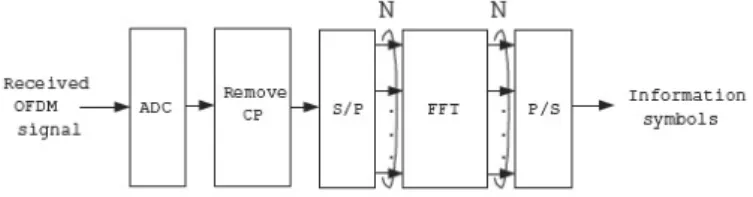
Figure 2: A typical OFDM demodulator.

2

Polynomial Cancellation Coded OFDM Systems

2.1

Introduction

Figure 2.1.1 plots a block diagram of a OFDM modulator where S/P and DAC are used to denote serial-to-parallel converter and digital-to-analog converter, respectively. The informa-tion symbols are used to modulate subcarriers vi N-points inverse discrete Fourier Transform (IDFT). The output of the IDFT (IFFT) block is converted to a serial complex block and a cyclic pre…x(CP) is added to each block. The total duration of an OFDM symbol (frame) is equal to the length of the CP plus that of the IDFT symbol block. The CP is a copy of the tail part of the time-domain OFDM block and is attached to the front of the block. As long as the duration of the CP is longer than the channel impulse response, inter symbol interference (ISI) can be eliminated by the receiver through frequency domain excision.

An OFDM demodulator is shown in Figure 2.1.2. Based on the timing (frame) recovery subsystem output, the baseband receiver removes the CP part, takes discrete Fourier trans-form (DFT) on the remaining part and then compensate for the CFO and channel e¤ect using information given by the frequency synchronization and channel estimation units before mak-ing decision on symbols modulated on each subcarriers, if no soft-decision channel decodmak-ing is needed. Parallel-to-serial conversion can be performed either before or after making symbol decision (detection).

Consider a frequency selective fading channel associated with an OFDM system with N sub-carriers. The frequency domain signal at the receiver at the kth subcarrier,Yk, is given by

Yk = S0Xk+ N 1

X

l=0;l6=k

Sl kXl+ nk; k = 0; 1; :::; N 1

Where nk is a complex additive white Gaussian noise(AWGN) sequence and Ykrepresents

the symbol carried by the kth subcarrier. Besides, Sl k = sin( (l + k)) N sin _N(l + k) exp j (1 1 N)(l + k)

is the ICI coe¢ cient.

Moreover, consider a frequency selective fading channel associated with an OFDM system,

Yk= S0HkXk+ N_X1 l=0;l6=k

Sl kHlXl+ nk; k = 0; 1; :::; N 1

Hl is the channel frequency response at the kth subcarrier.

2.3

Polynomial Cancellation Coding

The main idea of polynomial cancellation coding is to modulate one data symbol onto a group of subcarriers with prede…ned weighting coe¢ cients. By doing so, the ICI signals generated within a group can be “self-cancelled” each other.

2.3.1 Overview

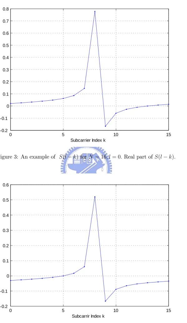
It has been shown in Figure1and Figure2 that both real and imaginary parts of the ICI coe¢ cient are gradually changed with respect to the subcarrier index.It’s worthwhile to notice that although the peak the desired signal located is not smooth with respect to the neighboring index, but in our ASR and SSR scheme, we will extract the peak signal for CFO estimation and make use of gradually changed property of the subcarriers with only even k.

We will introduce these polynomial cancellation coding schemes : ASR(adjacent data-conversion method,1996)

0 5 10 15 -0.2 -0.1 0 0.1 0.2 0.3 0.4 0.5 0.6 0.7 0.8 Subcarrier Index k

Figure 3: An example of S(l k)for N = 16; l = 0: Real part of S(l k):

0 5 10 15 -0.2 -0.1 0 0.1 0.2 0.3 0.4 0.5 0.6 Subcarrir Index k

2.3.2 ASR (adjacent data-conversion method)

over AWGN Channel From Figure 1 and Figure 2, for the majority of (l k)values, the di¤erence between Sl k and Sl k+1 is very small.

If a data pair (X0; X0) is modulated onto two adjacent subcarriers (k; k + 1) ; then the

ICI signals generated by subcarrier k will be cancelled out signi…cantly by the ICI generated by subcarrier (k + 1).

Therefore, the data block will be X = X0; X0; X1; X1; :::; XN

2 1; X N

2 1 . We name

this as modulation scheme of PCC. The received signal on subcarrier becomes

Yk = N_X2 l=0;l even

(Sl k Sl k+1) Xl+ nk; k = 0; 1; :::; N 1

And on subcarrier k + 1 becomes

Yk+1 = N_X2 l=0;l even

(Sl k 1 Sl k) Xl+ nk+1

In such a case, the ICI coe¢ cient is denoted as

Sl k = Sl k Sl k+1

By combining the received samples at the receiver, the e¤ective coe¢ cients are made to be small. It can be represented as

Yk = Yk Yk+1 = N_X2 l=0;l even (2Sl k Sl k+1 Sl k 1) Xl+ nk nk+1 = (2S0 Sl k+1 Sl k 1) Xk + N 2 X l=0;l even;l6=k (2Sl k Sl k+1 Sl k 1) Xl+ nk nk+1

The corresponding ICI coe¢ cient then becomes

S" = 2Sl k Sl k+1 Sl k 1

Besides, we name this as demodulation scheme of PCC.

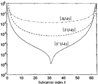
Figure 5: A comparison between S(l k); S0(l k)and S"_{(l k); N = 64:}

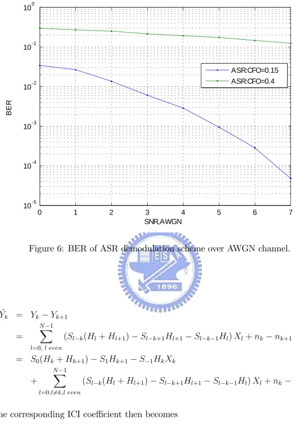
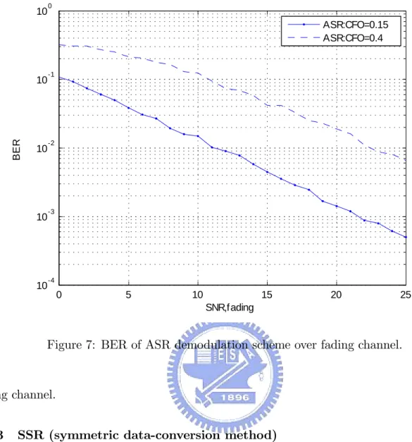
CFO increases to 0:4, the BER curve almost ‡ows. It shows that when CFO is large, the PCC can only eliminate ICI to a certain extent.

Over Fading Channel For ASR over fading channel, similarly, consider the data block X = X0; X0; X1; X1; :::; XN

2 1; X N

2 1 .The received signal on subcarrier becomes

Yk= N_X1 l=0; l even

(Sl kHl Sl k+1Hl+1) Xl+ nk; k = 0; 1; :::; N 1

where Hl is the channel frequency response at the k th subcarrier. And on subcarrier k + 1

becomes

Yk+1 = N_X1 l=0; l even

(Sl k 1Hl Sl kHl+1) Xl+ nk+1

In such a case, the ICI coe¢ cient is denoted as

Sl k = Sl kHl Sl k+1Hl+1

By combining the received samples at the receiver, the e¤ective coe¢ cients are made to be small. It can be represented as

0 1 2 3 4 5 6 7 10-5 10-4 10-3 10-2 10-1 100 SNR,AWGN BER ASR:CFO=0.15 ASR:CFO=0.4

Figure 6: BER of ASR demodulation scheme over AWGN channel.

Yk = Yk Yk+1 = N_X1 l=0; l even (Sl k(Hl+ Hl+1) Sl k+1Hl+1 Sl k 1Hl) Xl+ nk nk+1 = S0(Hk+ Hk+1) S1Hk+1 S 1HkXk + N_X1 l=0;l6=k;l even (Sl k(Hl+ Hl+1) Sl k+1Hl+1 Sl k 1Hl) Xl+ nk nk+1

The corresponding ICI coe¢ cient then becomes

S" = Sl k(Hl+ Hl+1) Sl k+1Hl+1 Sl k 1Hl

Figure 3 shows the amplitude comparison of jSl kj ; Sl k ;and Sl k" for N = 64 and

= 0:3over AWGN channel. Notice the logarithmic scale on the vertical axis.For the majority of (l k)values, Sl k is much smaller than jSl kj , and the Sl k" is even smaller then

Sl k .Thus, the ICI signals become smaller when applying the ASR scheme.

0 5 10 15 20 25 10-4 10-3 10-2 10-1 100 SNR,f ading BER ASR:CFO=0.15 ASR:CFO=0.4

Figure 7: BER of ASR demodulation scheme over fading channel.

fading channel.

2.3.3 SSR (symmetric data-conversion method)

Over AWGN Channel The other feature of the ICI coe¢ cients resulting from CFO error is that they are approximately symmetric. For the same modulated symbols with opposite polarity are transmitted on subcarrier k and (N k 1) , and this is the key idea used in SSR scheme to reduce the ICI.

Then, the data block becomes X = X0; X1; :::; XN

2 1; X N

2 1; X1; X0 .

We name this as modulation scheme of PCC. The received signal on subcarrier The received signal on subcarrier becomes

Yk = N 2 1 X l=0 (Sl k SN 1 l k) Xl+ nk; k = 0; 1; :::; N 1

0 1 2 3 4 5 6 7 10-5 10-4 10-3 10-2 10-1 100 SNR(dB) BER SSR:CFO=0.15 SSR:CF0=0.4

Figure 8: BER of SSR over AWGN channel.

YN 1 k = N 2 1 X l=0;l6=k Sl (N 1 k) S (l k) Xl+ nN 1 k

The decision variable at the receiver becomes

Yk = Yk YN k 1 = SN 1 S (N 1) Xk + N 2 1 X l=0;l6=k Sl k SN 1 k l Sl (N 1 k) S (l k) Xl+ nk nN 1 k

We name this as demodulation scheme of PCC.

From Figure 4, we can see that for small CFO of 0:15, SSR performs well. However, if CFO increases to 0:4, the BER curve almost ‡ows. It shows that when CFO is large, the PCC can only eliminate ICI to a certain extent.

0 5 10 15 20 25 10-3 10-2 10-1 100 SNR(dB) BER SSR:CF0=0.15 SSR:CF0=0.4

Figure 9: BER of SSR over fading channel.

The received signal on subcarrier The received signal on subcarrier becomes

Yk= N 2 1 X l=0 (Sl kHl SN 1 l kHN 1 l) Xl+ nk; k = 0; 1; :::; N 1

where Hl is the channel frequency response at the kth subcarrier. And on subcarrier

N 1 k becomes YN 1 k = N 2 1 X l=0;l6=k Sl (N 1 k)Hl S (l k)HN 1 l Xl+ nN 1 k

The decision variable at the receiver becomes

Yk = Yk YN k 1 = S0(Hk+ HN 1 K) S 2k+N 1HN 1 k S2k (N 1)Hk Xk + N 2 1 X l=0;l6=k Sl kHl SN 1 k lHN 1 l Sl (N 1 k)Hl+ S (l k)HN 1 l Xl+ nk nN 1 k

From Figure 4, we can see that the PCC can only eliminate ICI to a certain extent over fading channel.

3

CFO Estimation for ASR of Polynomial Cancellation

Coding

3.1

Modulation Scheme over AWGN Channel

The data block will be X = X0; X0; ::; XN

2 1; X N 2 1 : Recall that Yk = N_X2 l=0;l even (Sl k Sl k+1) Xl+ nk; k = 0; 2; :::; N 2

With Xk is derived from ICI self-cancellation scheme, and is deterministic.

According to the "Central Limit Theory", we approximate

N_X2 l=0;l even;l6=k

(Sl k Sl k+1) Xl=0~

Sum up Yk for k = 0; 2; :::; N 2;then E[Yk] becomes

E[Yk] ~=E[(S0 S1)Xk] + E[nk]; k = 0; 2; :::; N 2

When N is large, E[nk] ~=0 Then, 2 N N_X2 k=0;k even Yk Xk ~ =S0 S1 Denote ( ) = S0 S1

Then, the estimated ^ will be

^ = arg min ( ) 2 N N_X2 k=0;k even Yk Xk !

Next, we will discuss the real and imaginary parts of ( ) respectively. We will deonote the real part of a variable X as Re fXg, and the imaginary part of a variable X as Im fXg :

Since l k = 0, S0 = sin( ) N sin(_N )exp(j ) When N is large,sin(_N ) ~=_N Then S0 =~ sin( ) N_N exp(j ) ~ = sin( )exp(j ) Then, Re_fS0g ~= Re sin ( ) exp(j ) = sin ( ) cos ( ) = sin(2 ) 2 = sinc( )

Next, with l k = 1, and N is large.

S1 = sin( ( + 1)) N sin(_N( + 1))exp(j ( + 1)) ~ = sin( ( + 1)) ( + 1) exp(j ( + 1))

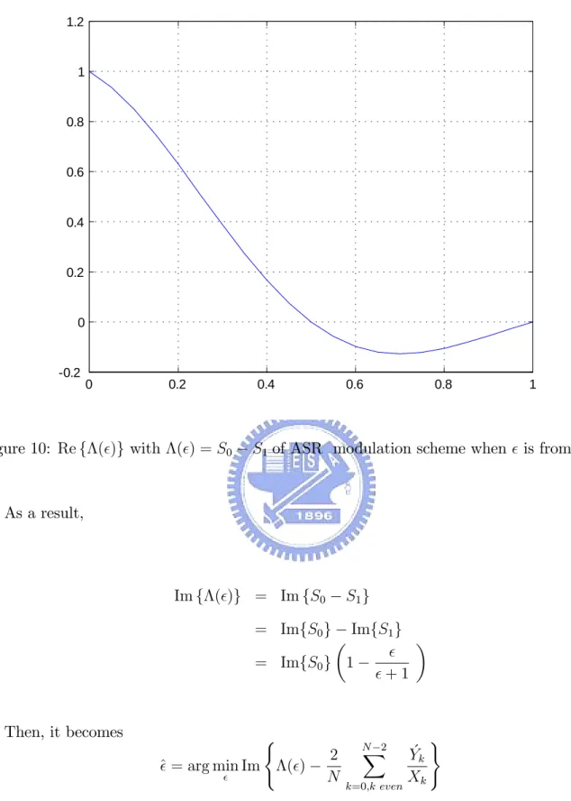
Re_fS1g ~= Re sin( ( + 1)) ( + 1) exp(j ( + 1)) = sin( ( + 1)) cos( ( + 1)) ( + 1) = sin(2 ( + 1)) 2 ( + 1) = sin(2 ) 2 2 2 ( + 1) = Re_fS0g ( + 1) As a result, Re_{f ( )g = Re fS}0 S1g = Re_fS0g RefS1g = Re_fS0g 1 + 1 Then, ^ = arg min Re ( ( ) 2 N N_X2 k=0;k even Yk Xk )

Next, consider the imaginary parts of ( ):

Im_fS0g ~= Im sin ( ) exp(j ) = sin ( )sin ( ) Im_fS1g = Im sin( ( + 1)) ( + 1) exp(j ( + 1)) = sin( ( + 1)) sin( ( + 1)) ( + 1) = sin( ) sin( ) ( + 1) = Im_fS0g ( + 1)

0 0.2 0.4 0.6 0.8 1 -0.2 0 0.2 0.4 0.6 0.8 1 1.2

Figure 10: Re f ( )g with ( ) = S0 S1of ASR modulation scheme when is from 0 to 1.

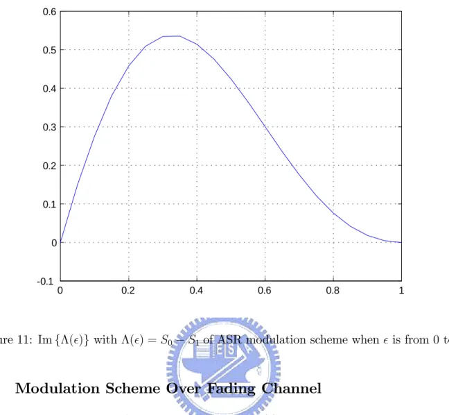
As a result, Im_{f ( )g = Im fS}0 S1g = Im_fS0g ImfS1g = Im_fS0g 1 + 1 Then, it becomes ^ = arg min Im ( ( ) 2 N N 2 X k=0;k even Yk Xk )

Refer to Figure 8 and Figure 9. Consider two regions of . The …rst region is from 0 to 0:5, and the second region is from 0:5 to 1. For the …rst region, Re f ( )g is one-to-one mapping, but Im f ( )g is not . For the second region, neither Re f ( )g nor Im f ( )g is one-to-one mapping. Therefore, we will use Re f ( )g to estimate CFO for in the range of 0 to 0:5.

0 0.2 0.4 0.6 0.8 1 -0.1 0 0.1 0.2 0.3 0.4 0.5 0.6

Figure 11: Im f ( )g with ( ) = S0 S1of ASR modulation scheme when is from 0 to 1.

3.2

Modulation Scheme Over Fading Channel

Consider transmission over fading channel and apply ASR. The received signal on subcarrier becomes Yk = Yk Yk+1 = (S0(Hk+ Hk+1) S1Hk+1 S 1Hk) Xk + N_X1 l=0;l6=k;l even (Sl k(Hl+ Hl+1) Sl k+1Hl+1 Sl k 1Hl) Xl+ nk nk+1

wherer Hl; l = 0; 1; :::; N 1 is the N point FFT of the delay pro…le. With Xk is derived

from ICI self-cancellation scheme, and Hl is perfect known.

Applying the Central Limit Theorem, we try to approximate

N 1

X

l=0;l6=k;l even

(Sl k(Hl+ Hl+1) Sl k+1Hl+1 Sl k 1Hl) Xl+ nk nk+1=0~

Yk = Yk Yk+1 ~ = (S0(Hk+ Hk+1) S1Hk+1 S 1Hk) Xk Then E h Yk i ~ = E [(S0(Hk+ Hk+1)) Xk] ~ = S0(Hk+ Hk+1)E [Xk] ; k = 0; 2; :::; N 2 EhYk i E [Xk] ~ = S0(Hk+ Hk+1) S1Hk+1 S 1Hk 2 N N_X2 k=0 Yk Xk ~ = S0(Hk+ Hk+1) S1Hk+1 S 1Hk ; k = 0; 2; :::; N 2 Denote ( ) = S0(Hk+ Hk+1) S1Hk+1 S 1Hk

Then ,the estimated ^ will be

^ = arg min ( ) 2 N N_X2 k=0;k:even Yk Xk !

3.3

Demodulation Scheme over AWGN Channel

Here we use ASR, and make use of the PCC demodulation scheme. The data block will be X = X0; X0; X1; X1; :::; XN 2 1; X N 2 1 : Recall that Yk = (2S0 S1 S 1) Xk + N 2 X (2Sl k Sl k+1 Sl k 1) Xl+ nk nk+1

With Xk is derived from ICI self-cancellation scheme, and is deterministic.

According to the "Central Limit Theory", we approximate

N_X2 l=0;l even;l6=k

(2Sl k Sl k+1 Sl k 1) ~=0

Since both nk is and nk+1 are AWGN noise, then nk nk+1 is also AWGN noise.

Sum up Yk for k = 0; 2; :::; N 2;then E[Yk] becomes

E[Yk] ~=E[(2S0 S1 S 1)Xk] + E[nk nk+1]; k = 0; 2; :::; N 2

When N is large, E[nk nk+1] ~=0 Then, 2 N N_X2 k=0;k:even Yk Xk ~ =2S0 S1 S 1 Denote ( ) = 2S0 S1 S 1

Then, the estimated ^ will be

^ = arg min ( ) 2 N N_X2 k=0;k:even Yk Xk ! Recall that Re_fS0g ~= sin(2 ) 2 = sinc( ) And Re_fS1g = RefS0g ( + 1)

With l k = 1, and N is large. S 1 = sin( ( 1)) N sin(_N( 1))exp(j ( 1)) = sin( ( + 1)) ( + 1) exp(j ( 1)) Then, Re_fS 1g = Re sin( ( 1)) ( 1) exp(j ( 1)) = sin( ( 1)) cos( ( 1)) ( 1) = sin(2 ( 1)) 2 ( 1) = sin(2 ) 2 2 2 ( 1) = Re_fS0g ( 1) As a result, Re_{f ( )g = Re f2S}0 S1 S 1g = 2 Re_fS0g RefS1g RefS 1g = Re_fS0g 2 + 1 1 Then, ^ = arg min Re ( ( ) N_X2 k=0;k:even Yk Xk )

Next, consider the imaginary parts of ( ).

Im_fS0g ~=

sin ( )

sin ( )

Im_fS1g = ImfS0g

Then, Im_fS 1g = Im sin( ( 1)) ( 1) exp(j ( 1)) = sin( ( 1)) sin( ( 1)) ( 1) = sin( ) sin( ) ( 1) = sin( ) sin( ) ( 1) = Im_fS0g ( 1) As a result, Im_{f ( )g = Im f2S}0 S1 S 1g = 2 Im_fS0g ImfS1g ImfS 1g = Im_fS0g 2 + 1 1 Then, ^ = arg min Im ( ( ) 2 N N_X2 k=0;k:even Yk Xk )

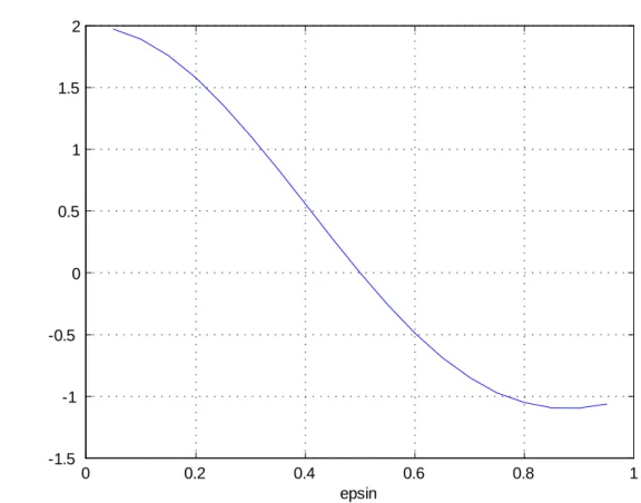
Refer to Figure 10 and Figure 11. Consider two regions of . The …rst region is from 0 to 0:5, and the second region is from 0:5 to 1. For the …rst region, Re f ( )g is one-to-one mapping, but Im f ( )g is not . For the second region, neither Re f ( )g nor Im f ( )g is one-to-one mapping. Therefore, we will use Re f ( )g to estimate CFO for in the range of 0 to 0:5.

3.4

Demodulation Scheme Over Fading Channel

Consider transmission over fading channel and apply ASR. The received signal on subcarrier becomes

0 0.2 0.4 0.6 0.8 1 -1.5 -1 -0.5 0 0.5 1 1.5 2 epsin

Figure 12: Re f ( )g with ( ) = 2S0 S1 S 1 of ASR demodulation scheme when is from

0 0.2 0.4 0.6 0.8 1 0 0.2 0.4 0.6 0.8 1 1.2 1.4 1.6 1.8 epsin

Figure 13: Im f ( )g with ( ) = 2S0 S1 S 1 of ASR demodulation scheme when is from

Yk = Yk Yk+1 = (S0(Hk+ Hk+1) S1Hk+1 S 1Hk) Xk + N 1 X l=0;l6=k;l even (Sl k(Hl+ Hl+1) Sl k+1Hl+1 Sl k 1Hl) Xl+ nk nk+1

wherer Hl; l = 0; 1; :::; N 1 is the N point FFT of the delay pro…le. With Xk is derived

from ICI self-cancellation scheme, and Hl is perfect known.

Applying the Central Limit Theorem, we try to approximate

N_X1 l=0;l6=k;l even

(Sl k(Hl+ Hl+1) Sl k+1Hl+1 Sl k 1Hl) Xl+ nk nk+1=0~

Besides, nk nk+1 is gaussian with zero mean.Then Yk becomes

Yk = Yk Yk+1 ~ = (S0(Hk+ Hk+1) S1Hk+1 S 1Hk) Xk Then E h Yk i ~ = E [(S0(Hk+ Hk+1)) Xk] ~ = S0(Hk+ Hk+1)E [Xk] ; k = 0; 2; :::; N 2 EhYk i E [Xk] ~ = S0(Hk+ Hk+1) S1Hk+1 S 1Hk 2 N N_X2 k=0 Yk Xk ~ = S0(Hk+ Hk+1) S1Hk+1 S 1Hk ; k = 0; 2; :::; N 2 Denote ( ) = S0(Hk+ Hk+1) S1Hk+1 S 1Hk

^ = arg min ( ) 2 N N_X2 k=0;k:even Yk Xk !

4

CFO Estimation for SSR of Polynomial Cancellation

Coding

4.1

Modulation Scheme Over AWGN Channel

Here we use SSR. The data block will be X = X0; X1::; XN

2 1; X N 2 1; X1; X0 : Recall that Yk = N 2 1 X l=0 (Sl k SN 1 l k) Xl+ nk; k = 0; 1; :::; N 2 1

With Xk is derived from ICI self-cancellation scheme, and is deterministic.

According to the "Central Limit Theory", we approximate

N 2 1

X

l=0;l6=k;

(Sl k SN 1 l k) ~=0

Sum up Yk for k = 0; 1; :::;N₂ 1;then E[Yk] becomes

E[Yk] ~=E[(S0 SN 1)Xk] + E[nk]; k = 0; 1; :::;

N 2 1 When N is large, E[nk] ~=0 Then, 2 N N 2 1 X k=0 Yk Xk ~ =S0 SN 1 Denote ( ) = S0 SN 1

Then, the estimated ^ will be

^ = arg min 0 @ ( ) 2 N N 2 1 X k=0 Yk Xk 1 A

0 0.2 0.4 0.6 0.8 1 -1.5 -1 -0.5 0 0.5 1 1.5 CFO

Figure 14: Re f ( )g with ( ) = S0 SN 1 of SSR modulation scheme when is from 0 to

1.

Refer to Figure 12 and Figure 13, both Re f ( )g and Im f ( )g are not strickly one-to-one mapping either when epsin is from 0 to 0:5 or when epsin is from 0 to 1. We will use Im_{f ( )g to estimate CFO in the simulation.}

4.2

Modulation Scheme Over Fading Channel

Consider transmission over fading channel and apply SSR. The received signal on subcarrier becomes Yk= N 2 1 X l=0 (Sl kHl SN 1 l kHN 1 l) Xl+ nk; k = 0; 1; :::; N 2 1

wherer Hl; l = 0; 1; :::; N is the N point FFT of the delay pro…le. With Xk is derived from

ICI self-cancellation scheme, and Hl is perfect known.

Applying the Central Limit Theorem, we try to approximate

N 2 1

X

l=0;l6=k

0 0.2 0.4 0.6 0.8 1 0 0.2 0.4 0.6 0.8 1 1.2 1.4 1.6 1.8 CFO

Figure 15: Im f ( )g with ( ) = S0 SN 1 of SSR modulation when is from 0 to 1.

Then E [Yk] ~=E [(S0Hl SN 1HN 1 k) Xk] E [Yk] E [Xk] ~ = S0Hl SN 1HN 1 k 2 N N 2 1 X k=0 Yk Xk ~ = S0Hl SN 1HN 1 k ; k = 0; 1; :::; N 2 1 Denote ( ) = S0Hl SN 1HN 1 k

Then ,the estimated ^ will be

^ = arg min 0 @ ( ) 2 N N 2 1 X k=0 Yk Xk 1 A

4.3

Demodulation Scheme Over AWGN Channel

Here we use SSR, and make use of the PCC demodulation scheme. The data block will be X = X0; X1::; XN 2 1; X N 2 1; X1; X0 : Recall that Yk = 2S0 SN 1 S (N 1) Xk + N 2 1 X l=0;l6=k Sl k SN 1 k l Sl (N 1 k) S (l k) Xl+ nk nN 1 k

With Xk is derived from ICI self-cancellation scheme, and is deterministic.

According to the "Central Limit Theory", we approximate

N 2 1

X

l=0;l6=k

Sl k SN 1 k l Sl (N 1 k) S (l k) =0~

Since both nk is and nk+1 are AWGN noise, thennk nN 1 k is also AWGN noise.

Sum up Yk for k = 0; 1; :::;N₂ 1;then E[Yk] becomes

E[Yk] ~=E[(2S0 SN 1 S (N 1))Xk] + E[nk nk+1]; k = 0; 1; :::;

N 2 1 When N is large, E[nk nN 1 k] ~=0 Then, 2 N N 2 1 X l=0;l6=k Yk Xk ~ =2S0 SN 1 S (N 1) Denote ( ) = 2S0 SN 1 S (N 1)

Then, the estimated ^ will be

^ = arg min 0 @ ( ) 2 N N 2 1 X l=0;l6=k Yk Xk 1 A

0 0.2 0.4 0.6 0.8 1 -1.5 -1 -0.5 0 0.5 1 1.5 CFO

Figure 16: Re f ( )g with ( ) = 2S0 SN 1 S (N 1)of SSR demodulation when is from

0 to 1.

Refer to Figure 14 and Figure 15, both Re f ( )g and Im f ( )g are not strickly one-to-one mapping either when epsin is from 0 to 0:5 or when epsin is from 0 to 1. We will use Im_{f ( )g to estimate CFO in the simulation.}

4.4

Demodulation Scheme Over Fading Channel

Consider transmission over fading channel and apply SSR. The received signal on subcarrier becomes Yk = Yk YN k 1 = S0(Hk+ HN 1 K) S 2k+N 1HN 1 k S2k (N 1)Hk Xk + N 2 1 X l=0;l6=k Sl kHl SN 1 k lHN 1 l Sl (N 1 k)Hl+ S (l k)HN 1 l Xl+ nk nN 1 k

wherer Hl; l = 0; 1; :::; N is the N point FFT of the delay pro…le. With Xk is derived from

0 0.2 0.4 0.6 0.8 1 0 0.2 0.4 0.6 0.8 1 1.2 1.4 1.6 1.8 CFO

Figure 17: Im f ( )g with ( ) = 2S0 SN 1 S (N 1) of SSR demodulation when is from

Applying the Central Limit Theorem, we try to approximate

Sl kHl SN 1 k lHN 1 l Sl (N 1 k)Hl+ S (l k)HN 1 l =0~

Besides, nk nk+1 is gaussian with zero mean.Then the received signal becomes

Yk = Yk YN k 1 ~ = S0(Hk+ HN 1 K) S 2k+N 1HN 1 k S2k (N 1)Hk Xk Then EhYk i ~ =E S0(Hk+ HN 1 K) S 2k+N 1HN 1 k S2k (N 1)Hk Xk EhYk i E [Xk] ~ = S0(Hk+ HN 1 K) S 2k+N 1HN 1 k S2k (N 1)Hk 2 N N 2 1 X k=0 Yk Xk ~ = S0(Hk+ HN 1 K) S 2k+N 1HN 1 k S2k (N 1)Hk ; k = 0; 1; :::;N 2 1 Denote ( ) = S0(Hk+ HN 1 K) S 2k+N 1HN 1 k S2k (N 1)Hk

Then ,the estimated ^ will be

^ = arg min 0 @ ( ) 2 N N 2 1 X k=0 Yk Xk 1 A

0.05 0.1 0.15 0.2 0.25 0.3 0.35 0.4 0.45 0.5 10-7 10-6 10-5 10-4 10-3 10-2 10-1 100 CFO MSE ASR modulation ASR demodulation SSR modulation SSR demodulation

Figure 18: Comparisons of MSE by di¤erent schemes of PCC over AWGN channel at SNR=3dB.

5

Simulation Results and Discussion

The followings are the MSE (mean square error) of estimates CFOs. For fading channel, we use the vehicular pro…le of IEEE 802.16m.The demoulation scheme performs better than the modulation one, as shown in Figure 3. Meanwhile, ASR performs better than SSR in the estimation of CFO over AWGN channel.

However, when CFO is small, ie, smaller than 0.15, ASR doesn’t do well compared with SSR. Recall Figure 13 and Figure 15, the imaginary part of desired signal is small when CFO is small. Thus the small desired signal will be a¤ected easily by noise, and results in worse performance.In Figure 17 the modulation of ASR performs better than others. However, the demodulation scheme performs worse than modulation scheme. The reason is that when channel is selective, the subtraction of the desired signal will enhance the ICI term. Besides, Figure 17 also shows that the SSR deals with the selectivity of channel better than ASR.

0.05 0.1 0.15 0.2 0.25 0.3 0.35 0.4 0.45 0.5 10-6 10-5 10-4 10-3 10-2 10-1 100 CFO MSE ASR modulation ASR demodulation SSR modulation SSR demodulation

Figure 19: Comparisons of MSE by di¤erent schemes of PCC over fading channel at SNR=25dB.

6

Conclusion

In OFDM systems, a carrier frequency o¤set (CFO) between the transmitter and receiver will results in ICI and thus destroy the orthogonality of the subcarrier and degrades the performance. ICI leads to attenuation and phase rotation of desired signal on each subcarrier. These impairments have already motivated several studies to …nd solutions. Among the several ICI reduction schemes, ICI self-cancellation or polynomial cancellation coding (PCC) scheme has received much attention due to its simplicity and its high robustness to frequency o¤set errors. However, for large CFO, PCC can only eliminate ICI to a certain extent. Thus, we propose new methods of PCC based CFO estimation to eliminate ICI for either low or high CFOs. First, we use PCC as precoding scheme and get the initial decoded data. Then CFO estimation is done by making use of the decode data. CFO estimation and compensation from PCC can overcome the drawback of PCC that only a certain part of ICI can be eliminated when CFO is large.

Our methods show good performanceof CFO estimation and improve system performance. Besides, it’s easy to be realized in real systems due to low computation.

7

Bibliography

[1] R. Nee and R. Prasad, OFDMfor wireless multimedia communications.Artech House Publishers, Mar. 2000.

[2] T. Pollet, Mark Van Blade1 and Marc Moeneclaey, "BER sensitivity of OFDM systems to carrier frequency o¤set and wiener phase noise,"IEEE Trans. Commun.. vol. 43, pp. 191-193, FebruarylMarcWApril 1999.

[3] L. Tomba, "On the e¤ect of Wiener phase noise in OFDM systems.,"IEEE Trans. Commun., vol. 46, pp. 580-583, May 1998.

[4] C.-L. Liu, "Impacts of I/Q imbalance on QPSK-OFDM-QAM detection,"IEEE Trans. Consumer Electron., vol. 44, pp. 984-989, Aug. 1998.

[5] H. Shatiee and S. Fouladifard. "Calibration of IQ imbalance in OFDM transceivers," in IEEE ICC, vol. 3, pp. 2081-2085, May 2003.

[6] Y. H. Kim, I. Song, H. G. Kim, T. Chang, and H. Myung, "Performance analysis of a coded OFDM system in time-varying multipath Rayleigh fading channels." IEEE Trans. Eh. Technol., vol. 48, pp. 161&1615, Sept. 1999.

[7] Y. Zhao and S . G. HGggman. "Intercarrier interference self-cancellation scheme for OFDM mobile communication systems," IEEE Trans. Cummun. vol. 49. pp. 1185-1191, July 2001.

[8] 1. Armrong, ‘Analysis of new and existing methods of reducing intercarrier interfer-ence due to carrier frequency o¤set in OFDM," IEEE Trans. Cummun., vol. 47. pp. 365-369, Mar. 1999.

[9] K. Sathananthan, R. M. A. P. Rajatheva, and S. B. Slimane, "Cancellation technique to reduce intercarrier interference in OFDM," IEE Elect., Lett., vol. 36, pp. 2078 -2079, Dec. 2000.7.13 .

[10] R. A. Casas, S. L. Biracree, and A. E. Youtz, "Time domain phase noise correction for OFDM signals," IEEE Trans. Broadcast., vol. 48, pp. 230–236, Sept. 2002.

[11] S. Wu and Y. Bar-ness, "A phase noise suppression algorithm for OFDM based WLANs," IEEE Commun. Lett., vol. 6, pp. 535–537, Dec. 2002.

[12] G. Liu and W. Zhu, "Compensation of phase noise in OFDM systems using an ICI reduction scheme," IEEE Trans. Broadcast., vol. 50, pp.399–407, Dec. 2004.

with feedback for OFDM in wireless communication," in Proc. of IEEE Global Telecom. Conf., Nov. 2002, vol. 1, pp. 651–655.

[14] H. C.Wu and X. Huang, "Joint phase/amplitude estimation and symbol detection for wireless ICI self-cancellation coded OFDM systems," IEEE Trans. Broadcast., vol. 50, pp. 49–55, Mar. 2004.

[15] X. Huang and H. C.Wu, "Totally blind phase correction scheme for ICI self-cancellation coded OFDM systems," in Proc. 60th IEEE Vehicular Technology Conf., Sep. 2004, vol. 5, pp. 26–29.

[16] H. C.Wu, X. Huang, and D. Xu, "Pilot-free dynamic phase and amplitude estima-tions for wireless ICI self-cancellation coded OFDM systems," IEEE Trans. Broadcast., vol. 51, pp. 94–105, Mar. 2005.

[17] M. Luise and R. Reggiannini, "Carrier frequency acquisition and tracking for OFDM systems," IEEE Trans. Commun., vol. 44, no. 11, pp. 1590–1598, Nov. 1996.

[18] Miin-Jong Hao," Decision Feedback Frequency O¤set Estimation and Tracking for General ICI Self-Cancellation Based OFDM Systems",Broadcasting, IEEE Transactions on Volume 53, Issue 2, June 2007".

[19] P.H. Moose, "A technique for orthogonal frequency division multiplexing frequency o¤sets and Wiener phase noise," IEEE Trans. Commun., vol 43, pp.191-193, Feb./March/April 1995.