Option-based Capacity Planning for Semiconductor Manufacturing
Yi-Yu Liang and Yon-Chun ChouNational Taiwan University Taipei, Taiwan ychou@ntu.edu.tw
Abstract – Due to high cost of capacity investment, many semiconductor manufacturing companies have exhibited the need to pursuit innovative capacity plans and planning methods. In this paper, a case study of option-based capacity planning is presented. Three issues are addressed: estimation of production cost parameters, valuation of capacity, and analysis design . It is shown that the option-based approach, in long-term, could generate a capacity plan that requires less investment, but generates higher operating income.
1. INTRODUCTION
Capacity planning is crucial to corporate performance in the semiconductor industry but is very challenging. Figure 1 shows the installed capacity and output of a major manufacturing company over a period of 9 years. There are periods of severe over- and under-capacity. Due to high cost of capacity investment, corporate performance is necessarily impaired by such mismatches between demand and capacity. This phenomenon is not limited to any one company but is pervasive in the industry. Therefore, many companies have exhibited the need to pursuit innovative capacity plans and planning methods.
0 200 400 600 800 1000 1200 Q1 -9 4 Q3 -9 4 Q1 -9 5 Q3 -9 5 Q1 -9 6 Q3 -9 6 Q1 -9 7 Q3 -9 7 Q1 -9 8 Q3 -9 8 Q1 -9 9 Q3 -9 9 Q1 -0 0 Q3 -0 0 Q1 -0 1 Q3 -0 1 Q1 -0 2 Q3 -0 2 Installed Capacity Wafer Out Figure 1. Mismatch between capacity and output Capacity planning comprises many tasks (Table 1). Most of the studies in the literature address the problem of tool portfolio optimization. Swaminathan addresses the tool procurement decision over a planning horizon of multiple time periods [8]. The uncertainty of product demand is modeled by a set of demand scenarios. A large integer program is described that minimizes the expected stock-out cost over all demand scenarios. Barahona et al. describes a stochastic programming approach under demand uncertainty [2]. The tool purchase, wafer starts, and work assignment decisions are formulated as a large mixed-integer program. Ahmed uses multi-stage stochastic programming instead of two-stage stochastic programming to better model the flexibility of tool purchase in later time
periods bestowed by occurrence of new events [1]. The paper compares the relative merit between two-stage and multi-stage stochastic programming, and finds that the merit increases with the number of stages and the number of decision branches per stage. Christie and Wu describe a stochastic programming formulation for tool portfolio planning at the multiple-plant level [6].
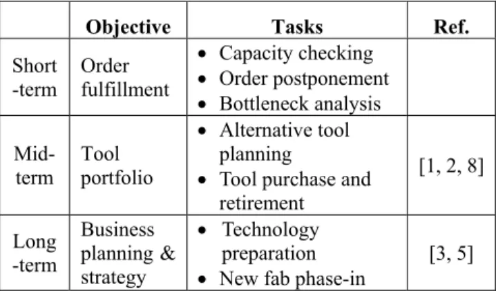
Objective Tasks Ref.
Short
-term Order fulfillment
• Capacity checking • Order postponement • Bottleneck analysis Mid-
term Tool portfolio
• Alternative tool planning
• Tool purchase and retirement [1, 2, 8] Long -term Business planning & strategy • Technology preparation
• New fab phase-in [3, 5] Table 1. Capacity planning tasks and methodologies A few papers address long-term or process issues related to capacity planning. The plant-sizing problem is addressed by Benavides et al. [3]. Product demand is assumed to follow a geometric Brownian motion process. The timing decisions are modeled as an optimal stopping problem. The paper shows that optimal trade-off between economics of scale, and flexibility can be reached by a sequential deployment of modular plants. Karabuk and Wu consider the coordination problem between production manager and marketing management in the same corporate organization, that is, to blend the two forces that drive the decisions on capacity planning [7]. Two types of uncertainties are modeled: one is capacity estimation and the other is demand volatility. Stochastic programming is used to solve the optimal capacity plan.
The basic logic of conventional capacity planning is to have sufficient capacity which will satisfy product demands. The goal is typically to maximize the profit. In this paper, it is shown that this logic is not necessary correct. This logic would be correct only if the demand could be predicted with certainty.
In this paper, a study of option-based capacity planning is presented using the data of Figure 1 and other relevant data. The basic idea of the option-based approach is that capacity decisions should include the option of waiting for more demand information to materialize [6], in addition to pursuing immediate capacity expansion to match demand forecasts that are rarely correct. Beside the conclusion section, the remainder of the papers has three parts.
77 0-7803-7894-6/03/$17.00 ©2003 IEEE.
Calibration of demand uncertainty is first described. This is followed by a model for the valuation of capacity. The model is then applied to the historical capacity trajectory of Figure 1 to evaluate the potential benefits of the option-based approach.
2. CALIBRATION OF UNCERTAINTY
The uncertainty in demand is the root cause of the problem facing capacity planning. There have been little studies on characterizing the uncertainty. The geometric Brownian motion (GBM) process has been used in [3] to model the demand process. In this paper, we analyze the suitability of BMP as a modeling tool using the demand phenomenon of Figure 1 as the case study. [Note that the wafer output can be considered as a one-side estimate of actual demand.] A GBM process is characterized by a diffusion equation:
t t t
t q dt q dw
dq =µ⋅ ⋅ +σ⋅ ⋅ where is the demand at time t, is the standard Wiener process, and
t q t
dw µ and σ are
the drift and variance parameters respectively. Following the method described in [8], the growth rate rt, can be estimated by )] ( ), )( 2 / [( ~ ) ln( ) ln(q q0 N 2 t t0 2t t0 rt= t − t µ−σ − σ −
and the drift and variance parameters can be estimated by
0 ˆ t t r s − =
σ
and 2 2 ˆ 0 ˆ σµ
= −t + t r where ∑ − − = ∑ = = = n t t r n t t r r n s n r r 1 2 1 ( ) ) 1 ( 1 ;The drift and variance parameters have the value of 0.2596 and 0.3339 respectively. Figure 2 shows some sample paths of the constructed model, which validate that the model can reasonably represent the variability of the underlying demand process. 0 400 800 1200 1600 2000 Q1 -9 4 Q3 -9 4 Q1 -9 5 Q3 -9 5 Q1 -9 6 Q3 -9 6 Q1 -9 7 Q3 -9 7 Q1 -9 8 Q3 -9 8 Q1 -9 9 Q3 -9 9 Q1 -0 0 Q3 -0 0 Q1 -0 1 Q3 -0 1 Q1 -0 2 Q3 -0 2 Sample Path-1 Sample Path-2 Sample Path-3 Sample Path-4 Historical Data
Figure 2: Sample paths of the demand process To facilitate numerical computation, the binominal model of Jarrow and Rudd [6] is then used to approximate the continuous demand process (Figure 3). In this model, the
possibilities of an increase or a decrease in demand are equal (Figure 3). 2 1 1 ; 2 1 ] ) exp[( ] ) exp[( 2 0 0 0 2 0 0 0 = − = ∆ − ∆ − = ⋅ = ∆ + ∆ − = ⋅ = − ∆ + + ∆ + p p t t q v q q t t q u q q t t t t t t t t σ σ µ σ σ µ 0 t t= t =t0 +∆t t=t0+2∆t 0 t q + ∆ + t t q0 − ∆ + t t q 0 −− ∆ + t t q0 2 − + ∆ + t t q0 2 + + ∆ + t t q0 2 p p − 1 p p − 1 p p − 1
Figure 3: The binominal tree of demand variation The value of capacity is dependent on future demand. In this study, we analyze the capacity trajectory of Figure 1 and evaluate the rationality of each capacity increment with the premise that the underlying demand process is GBM of the previous section.
3. VALUATION OF CAPACITY
Parameter estimation
The dominant cost item in semiconductor manufacturing is the depreciation of machines, equipment and facility. In this study, this cost is called (irreversible) fixed costs and all other costs are called variable costs. Note that by lumping overhead costs with other variable costs, this dichotomy classification is different from conventional cost accounting practice. We have analyzed historical data of total variable cost and capacity level. Figure 4 clearly exhibits a proportional relationship between total variable cost (vertical axis) and capacity level (horizontal axis). The variable production cost is estimated to be $659 per wafer.
0 100 200 300 400 500 600 700 800 0 200 400 600 800 1,000 1,200
Figure 4: Relationship between total variable cost and capacity level
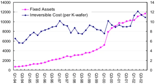
Another interesting finding in our data analysis shows that the irreversible cost per unit of capacity is fairly constant. Over the nine year period, the total fixed asset of the company increased by 10 folds but the ratio of capacity to fixed asset varying over a narrow range (Figure 5). It can be interpreted that for a factory generation (such as 200 mm wafer), this unit cost could be regarded as a constant. The significance of this finding is that the model of rationality analysis will have one less variable. From Figure 5, the average irreversible cost of capacity as measured by wafer per quarter is approximately $9,514.
0 2000 4000 6000 8000 10000 12000 14000 Q1 -9 4 Q3 -9 4 Q1 -9 5 Q3 -9 5 Q1 -9 6 Q3 -9 6 Q1 -9 7 Q3 -9 7 Q1 -9 8 Q3 -9 8 Q1 -9 9 Q3 -9 9 Q1 -0 0 Q3 -0 0 Q1 -0 1 Q3 -0 1 Q1 -0 2 Q3 -0 2 0 2 4 6 8 10 12 14 Fixed Assets
Irreversible Cost (per K-wafer)
Figure 5. Irreversible cost of unit capacity
Value in place
Given a realized demand at time t, the future demand will be represented as a binomial scenario tree. Let the current capacity be
c
0 and the capacity increment be ∆c . The effective capacity increment, ECI, can be expressed as]] 0 , max[ , [min[ )] , , ( [ ) , , ( 0 0 0 c q c E c c q f E c c q ECI t s t t s t t − ∆ = = ∆
where the expected value is computed over the scenario tree s. Let the deployment lead-time be d, the life time of capacity be l, p be the price and v be the variable cost. An irreversible cost is incurred for a capacity increment . The value in place for a capacity increment is the total operating profit, defined as revenue less variable cost, during its life time.
) ( c I ∆
c
∆
) , , ( ) ( ) , , ( 0 0 0 )) 0 ( ( 0 ) 0 ( , 0 c c q ECI v p e c c q V t t l d t d t t d t t r t t s t ∆ ⋅ ∑ ⋅ − = ∆ + + + = + − −The value of a capacity increment is its value in place subtracted by its irreversible cost.
The value of waiting, F , is the discounted value of deploying the capacity increment in the next period.
) ( , ts t ))]] ( ) , , ( ( )), ( ) , , ( [max[( ) exp( )) ( ) , , ( ( 0 ) ( , , 0 0 , 0 0 ) ( , ) 0 ( , 0 c I c c q V F c I c c q V E t r c I c c q V F t t s t s t t t s t t s t t s t t s t ∆ − ∆ ∆ − ∆ ⋅ ∆ − = ∆ − ∆ ∆ + ∆ +
Both sizing and timing of capacity decisions can be made based on the value of capacity and value of waiting. In general, the optimal capacity increment and the demand required to trigger a pre-specified capacity increment (Figure 6) occur at the point where the two quantities have equal value: )) ( ) , , ( ( ) ( ) , , ( 0 0, (0) , () 0 ) 0 ( , 0 q c c I c F V q c c I c Vt st t ∆ − ∆ = t st tst t ∆ − ∆ -200 -100 0 100 200 300 400 0 50 100 150 200
Value in Place - Irreversible Cost Value of Waiting
Figure 6. Optimal capacity increment 4. PERFORMANCE EVALUATION
Forecasting demand is a complicated business process. Because of the volatile nature of the semiconductor industry, the visibility of demand is also very dynamic. Sometimes there is very low visibility on the next quarter. Other times, there are significant backlogs so that the demand in term of workload is visible over the near future. Both cases must have occurred over the nine year period. In order to evaluate the rationality of the capacity trajectory, clever design of analysis is required.
Design of analysis
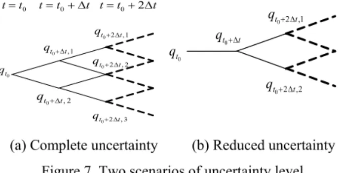
We have designed two boundary scenarios for rationality analysis. The first scenario assumes that the GBM model is a faithful representation of the demand process and no historical output data beyond the base period is utilized. This scenario is called the scenario of complete uncertainty. The other scenario assumes that the demand of the current and next time periods is reasonable available. But the demand beyond the next time period is full of uncertainty. This scenario is called the scenario of reduced uncertainty. These two scenarios will delineate the boundary in which the actual demand might fall.
Denote the demand scenario tree emanating from at time t as S . The demand tree for the complete uncertainty scenario is S , whereas that of the reduced uncertainty is . t q ) ( t t q ) ˆ ( t t q ˆ ( t+ t q S 1) 79
0 t t= t=t0+∆t t=t0+2∆t 0 t q 1 , 0 t t q +∆ 2 , 0 t t q +∆ 2 , 2 0 t t q+ ∆ 3 , 2 0 t t q+∆ 1 , 2 0 t t q+∆ 0 t q t t q0+∆ 1 , 2 0 t t q +∆ 2 , 2 0 t t q+ ∆
(a) Complete uncertainty (b) Reduced uncertainty Figure 7. Two scenarios of uncertainty level
The option-based model described in Section 3 has been applied to the two scenarios of analysis. A new capacity trajectory is generated following the option-based approach. Capacity increments are determined using the sizing rule and capacity decrements are taken directly from the historical capacity trajectory. The resultant two capacity trajectories are shown in Figure 8. It can be observed that both trajectories are more conservative than the historical trajectory. 0 200 400 600 800 1000 1200 Q1 -9 4 Q3 -9 4 Q1 -9 5 Q3 -9 5 Q1 -9 6 Q3 -9 6 Q1 -9 7 Q3 -9 7 Q1 -9 8 Q3 -9 8 Q1 -9 9 Q3 -9 9 Q1 -0 0 Q3 -0 0 Q1 -0 1 Q3 -0 1 Q1 -0 2 Q3 -0 2 Historical Practice Demand Complete Uncertainty Reduced Uncertainty
Figure 8. Trajectories of capacity increment The revenue, operating income and capacity cost of the two trajectories are compared with those of the historical
trajectory in Figure 9. Following the option-based approach, the capacity cost will be lower but the operational income will be higher by a ratio between 0.1% and 7.6%.
0 2 4 6 8 10 12 14 16 18 20 Historical Practice Complete Uncertainty Reduced Uncertainty Revenue Capacity Cost Operating Income
Figure 9. Income of capacity trajectories 5. CONCLUSIONS
In this paper, the rationality of capacity trajectory of a major semiconductor manufacturing company is analyzed
at the aggregate level. Our data analysis has produced useful findings on the relationship between capacity and total assets. It is shown that the option-based approach could generate a capacity plan that requires less investment, but generates higher operating income in the long term.
REFERENCES
[1] Shabbir Ahmed, “Semiconductor Tool Planning via Multi-stage Stochastic Programming,” Proc. of 2002 Int. Conference on Modeling and Analysis of Semiconductor Manufacturing, Tempe, Arizona, U.S.A., 153-157, Apr. 2002.
[2] Francisco Barahona, Stuart Bermon, Oktay Gunluk, and Sarah Hood, "Robust Capacity Planning in Semiconductor Manufacturing," Research Report RC22196, IBM, 2001.
[3] Dario L. Benavides, et al, “As Good as It Gets: Optimal Fab Design and Deployment,” IEEE Transactions on Semiconductor Manufacturing, Vol. 12, No. 3, 281-287, 1999.
[4] Avanish K. Dixit and Robert S. Pindyck, Investment
under Uncertainty, Princeton University Press, 1994.
[5] D. Gary Eppen, R. Kipp Martin, and Linus Schrage, “A Scenario Approach to Capacity Planning,” Operations Research, Vol.37, No. 4, 517-527, 1989.
[6] A. Robert Jarrow and Andrew Rudd, Option Pricing, Irwin, USA, 1983.
[7] Suleyman Karabuk; S. David Wu, “Coordinating Strategic Capacity Planning in the Semiconductor Industry” Technical Report 99T-11, Dept of IMSE, Lehigh University, 2001.
[8] J. M. Swaminathan, "Tool Capacity Planning for Semiconductor Fabrication Facilities under Demand Uncertainty," European Journal of Operations Research, Vol. 120, 545-558, 2000.
[9] Ruey S. Tsay, Analysis of Financial Time Series, New York, United States of America, John Wiley and Sons, Inc., 2002.
ACKNOLEDGEMENT
This study was partially supported by Semiconductor Manufacturing Corp. under grant 201-NJ-879 and National Science Council, Republic of China, under grants 90-2218-E-002-043 and 90-2128-E-002-042.
AUTHOR BIOGRAPHY
Y-C Chou received a Ph.D. degree form Purdue University in
1988. He is a professor and the director of the Institute of Industrial Engineering, National Taiwan University. His research interests include production and logistics systems design, production scheduling, and decision theory. His recent work focuses on semiconductor manufacturing and supply chain management.
Yi-Yu Liang received a M.S. degree in industrial engineering in
2003 and a dual B.B.A. degree in Finance and Accounting in 2001, both from National Taiwan University.
![Figure 2: Sample paths of the demand process To facilitate numerical computation, the binominal model of Jarrow and Rudd [6] is then used to approximate the continuous demand process (Figure 3)](https://thumb-ap.123doks.com/thumbv2/9libinfo/8860299.244887/2.918.508.798.130.408/figure-facilitate-numerical-computation-binominal-approximate-continuous-figure.webp)