以多相混合理論分析土石流運動模式(II)數值模擬

行政院國家科學委員會補助專題研究計畫成果報告

※ ※※※※※※※※※※※※※※※※※※※※※※※※

※

※

※

以多相混合理論分析土石流運動模式(II):數值模擬

※

※ Dynamic Models of Debris Flow Based on ※

※ Multi-phase Mixture Theory (II): Numerical Modeling ※

※

※

※ ※※※※※※※※※※※※※※※※※※※※※※※※

計畫類別：■個別型計畫

□整合型計畫

計畫編號：NSC 90－2211－E－151－007

執行期間：

90 年 08 月

01 日至

91 年

07

月

31 日

計畫主持人：黃立政 副教授

共同主持人：蕭達鴻 副教授

本成果報告包括以下應繳交之附件：

□赴國外出差或研習心得報告一份

□赴大陸地區出差或研習心得報告一份

□出席國際學術會議心得報告及發表之論文各一份

□國際合作研究計畫國外研究報告書一份

執行單位：國立高雄應用科技大學土木工程系

中

華

民

國

91

年

07

月

31

日

行政院國家科學委員會專題研究計畫成果報告

以多相混合理論分析土石流運動模式 (II): 數值模擬

Dynamic Models of Debr is Flow Based on Multi-phase Mixtur e Theor y (II):

Numer ical Modeling

計畫編號：NSC 90-2211-E-151-007

執行期限：90 年 08 月 01 日至 91 年 07 月 31 日

主 持 人：黃立政 副教授 國立高雄應用科技大學土木工程系

共同主持人：蕭達鴻 副教授 國立高雄應用科技大學土木工程系

E-mail:

[email protected]

一、中文摘要 本計畫嘗試以多相混合物理論推導描述土石 流運動之統御方程式; 將土石流視為礫石、細泥、 水及空氣四種相之混合物，由聯體力學之微觀平衡 方程式出發，利用平均原理，建立巨觀之平衡方程 式，分別描述包括質量、線動量、角動量、能量、 火商等守恆原理，再引入適當之本構方程式，可建 立以多相混合物理論為基礎之土石流運動統御方 程式；加上邊界條件及初始條件，構成適當之土石 流解析模式。本計畫進一步嘗試發展一個基於原始 變數表示式之邊界元素解法用以分析具低雷諾數 二維恆態不可壓縮黏性流場。將統御方程式中之非 線性對流項及二次簡應力項視為徹體力，由勞倫茲 反位定理可推導出包含邊界速度與邊界曳引力與 解域徹體力之積分方程式。採用恆態史托克流場之 基本解並進行迭代運算及面積積分，全部之邊界速 度及曳引力，內部點之速度、壓力、渦量、剪應力 等均可計算得出。流線函數亦可由波松方程式相應 之積分方程式求得。將邊界元素法應用於壁動引發 方形穴流之廣義黏塑性非牛頓型流體流場分析，結 果顯示在低雷諾數範圍內本法提供相當理想之數 值分析途徑。 關鍵詞：土石流、多相混合理論、非牛頓型流體、 數值模擬、邊界元素法。 Abstract

This paper is proposed to build the governing equations for analysis of debris flow based on the

multi-phase mixture theory. The debris flow is considered to be a mixture of four constituents, i.e., stone, mud, water and air. Starting from the microscopic balance equations based on the theory of continuum mechanics and averaging theorems, the macroscopic balance equations are first built up to represent the conservation of mass, linear momentum, angular momentum, energy and entropy. After the constitutive relations are employed, the governing equations for debris flows are obtained. Mathematical model is completed when appropriate boundary conditions and initial conditions are prescribed. Furthermore, a boundary element method for analysis of steady two-dimensional incompressible viscous flow with low Reynolds numbers based on primitive variable is presented. A generalized visco-plastic fluid model is employed as the constitutive law of debris flow. The convective terms and the quadratic velocity gradient terms in the equations of motions are treated as equivalent body forces. The boundary integral equations for velocities and tractions are first formulated and the associated kernel functions for internal velocities, velocity gradients, pressures, vorticities and shearing stresses are explicitly derived. Both domain integration and iterative process are required since nonlinear convective term is present. However, the incompressibility condition is satisfied exactly in the formulation and thus no artificial compressibility and/or penalty are required as in the finite difference and finite element methods. Stream function in the interior is evaluated via the integral equation associated with the Poisson equation. Computational results for the wall driven Generalized visco-plastic Non-Newtonian fluid flow in a square cavity depict that the boundary element method present here provides a convenient tool for numerical analysis of two-dimensional incompressible non-Newtonian viscous flows with low Reynolds numbers.

Keywords: Debris flow, multi-phase mixture theory,

1. Intr oduction

Disasters caused by debris flows often occur in Taiwan recently and there are many natural or manmade factors leading to these tremendous accidents [1,2]. Development of prevention techniques is obviously based on the understanding and analysis of the mechanical behavior of debris flow.

Debris flows are inherently non-Newtonian flows from the viewpoints of view of fluid mechanics, in which the rheological behavior is highly nonlinear and complicated. On the other hand, from the viewpoints of solid mechanics, debris flows are porous media filled with water, air and other slurries.

There have been a lot of flow models for analysis of mechanical characteristics of debris flow. Among these research works, the following models are useful and significant: the dilatant fluid model initiated by Bagnold (1954) and extended by Takahashi (1977); the Bingham fluid model, pseudo- or generalized visco-plastic fluid model such as those proposed by Chen (1986), O’Brien and Julien (1988), Chen et al. (1991), Julien and Lan (1991), etc.; Prandtl mixing-length model employed by Matsumura and Mizuyama (1990); modified turbulent flow model proposed by Yu and Chen(1990); a mixed-layer model proposed by Su et al (1993); a two-layer model, proposed by Ho and Chen (1997) in which an inertia sub-region and a viscous sub-region exist [3-13]. It has been found by experimental study that the Bingham fluid model is appropriate for mud flow while dilatant fluid model works well for stony flow in which dispersive stresses together with the viscous shear stresses play the same role in the rhelogical behavior of the debris flow.

Thus it is naturally to develop a rheological model based on the theory of multi-phase mixture, in which the debris flow is considered to be a mixture of four constituents, i.e., stone, mud, water and air. In the analysis of geophysical and geotechnical problems, theories of multi-phase mixture have been employed for a long time [14-19]. There are two basic points of view on the multi-phase mixture, i.e., the microscopic and the macroscopic, respectively. On the other hand, concept of effective stress has been employed by Terzaghi (1936) [20] and extended by Biot (1941, 1956) [21,22].

Once the constitutive relationship is built up we can theoretically evaluate the kinematic characteristics of debris flow along a slope such as velocity profile, mean velocity, plug velocity, momentum correction factor and energy correction factor, etc. Special cases for degenerating condition can also be obtained in a simple way.

Analysis of incompressible viscous flow is an old subject in the literature of fluid dynamics. Analytical solutions are rare and can only be obtained for physical problems possessing regular geometry and simple boundary conditions. In practical situation we often resort to numerical methods with which steady incompressible viscous flow governed by the

Navier-Stokes equations are considered. Among various methods for computational fluid dynamics (CFD), the finite difference methods (FDM) and finite element methods (FEM) are two famous numerical schemes [23,24]. There are three formulations for numerical analysis of the Stokes flow and more general the viscous flow governed by Navier-Stokes equations: (1) vorticity-stream function approach, (2) primitive variable (velocity-pressure) approach, and (3) vorticity-velocity approach. The disadvantages of (1) and (3) are the difficulties in appropriate prescription of boundary conditions for the vorticity while the approach (2) is associated with problem of satisfaction of the continuity equation. In FEM, various schemes have been developed such as mixed-FEM, penalty-FEM and multiplier-FEM, etc. [26,27]. These domain-type numerical schemes possess the following common disadvantages: (a) even velocity components are continuous, the pressures are often discontinuous from elemet to element, (b) infinite domain discretization is required for external flows, (c) no rigorous mathematical reasoning within the determination of artificial compressibility.

Recently, numerical methods based on boundary integral equations are widely applied to solid mechanics and fluid dynamics [28]. There are many research works on the applications of BEM to the numerical solutions of steady and incompressible Navier-Stokes equations such as Wu and Thompson [29], Mills [30], Bush and Tanner [31], Bush [32], Onishi et al. [33], Dargushi and Banerjee [34]. Specific applications of BEM to Stokes flow are discussed by Elliot et al. [35], Zhou and Pozrikids [36]. The main advantages of BEM are (a) only boundary of the physical domain should be discretized if the body force (such as gravitational force) is absent and thus domain integration is not required, (b) dimension of the problem is reduced by one and only contour integration is considered for a two-dimensional problem, and especially (c) kinematic conditions of incompressibility is satisfied in the fundamental solutions thus no artificial compressibility or penalty is required as in the FDM and FEM.

However, most of present BEM solvers for steady incompressible viscous flow are based on the vorticity-stream function or vorticity-velocity formulations. The disadvantages of modeling of boundary conditions of vorticity are still present as in the FDM and FEM. Recently, a BEM for steady two-dimensional Stokes flow based upon primitive variables (velocity-pressure) is developed by the author [38]. The boundary integral equations are derived from the original governing equations of steady Stokes flow, i.e., the continuity and momentum equations. The main unknowns are the boundary velocities and tractions and the boundary conditions can be imposed in a natural way. The integral equation representations for internal velocities, pressures, vorticities and shearing stresses related to the boundary velocities and tractions are formulated easily.

In this study the scheme is extended to steady incompressible viscous flow with low Reynolds number, i.e., the flow with convective accelerations. The kernels using in the integral equations of Stokes flow will be employed as the fundamental solutions for the current Navier-Stokes equations. Both iterative process and domain integration are required in the numerical method due to the presence of nonlinear terms in the governing equations. A numerical example of cavity flow using constant boundary elements and uniform internal cells will be employed to check the validity and efficiency of the BEM developed.

2. Gover ning Equations for Debr is Flow

2.1 Macr oscopic balance equations for debr is flow

The debris flow is considered to be a multi-phase mixture composed of four constituents, i.e., stone, mud, water and air. Thus the density of the mixture can be expressed as

α ρ α ηα ρ η ρ η ρ η ρ η ρ ∑ = = + + + = 4 1 a a w w m m g g (1)

where ρ_g,ρ_m,ρ_w,ρ_a denotes the density of stone, mud, water and air, respectively. It is obviously seen that 1 4 1 = ∑ = i ηα (2)

We have the following macroscopic balance equations in indicial form:

0 , ) ( = +η_αρ_α α α ρ α η α k k v Dt D (3a) 0 . − − = − α η_αρ_α α η_α α α α α ρ α η t_klk g_l T_l Dt l v D (4b) α α lk t kl t = (4c) 0 , , = − − − − α α ρ α η α α ρ α η α α α α α α ρ α η Q h k k q k l v kl t Dt E D (4d) α α ρ α η α θ α α ρ α η α θ α α α α ρ α η − qk _k − h = Γ Dt S D , ) ( (4e) subject to 0 4 1 = ∑ = α α ρ α η α Tl (4a) 0 ) ( 4 1 + = ∑ = α α α α ρ α ηα Tl vl Q (4b)

When the temperature in each phase is the same (isothermal condition), i.e.,

θ θ θ θ

θ_g = _m = _w= _a = (5) As a result, energy equations for each phase need not be considered. Rather a total energy equation obtained

as the sum of each phase energy equations will be

0 , ) ( , 4 1[ , = − − + ∑ = − h k k v E k k q k l v kl t Dt DE ρ α α α ρ α η α α α α ρ (6) where ∑ = = 4 1 α ρα α ρE E (7) and ∑ = = 4 1 α α α ρ ρh h (8)

2.2 Constitutive equations for debr is flow

The balance equations given in equations (3), (4) and (6) constitute equations in 73 unknowns, namely:

) 3 , 2 , 1 , ; 34 , 2 , 1 ( , , , , , , , , , , = = k l S k q E k T kl t k v a w m α α α α α α θ α α ρ η η η (9) However, some dependent variables can be related to others based on the so-called constitutive relations of each phase of the constituents.

(i) If the solid phase is assumed to be isotropic elastic, then ) , ( 2 Se_klS S g m kl S mn e S kl f p S S kl t =−η δ +λ δ + µ = (10a) where kl

δ is the Kronecker delta, S

kl

e is the tensor of the rate of deformation of solid phases, λ ,S µS are Lame constants of solid phases.

(ii) For Newtonian fluid (such as water and air phases): ) , ( 2 fe_klf f wa kl f mm e f kl f p f kl t =− δ +λ δ + µ = (10b) where f kl

e is the tensor of the rate of deformation of fluid phases, λ ,f µf are Lame constants of fluid phases.

(iii) If the mud is assumed to be a Bingham fluid:

m l k v m m Y m kl t =τ +µ _, (10c) in which τ ,_{Y µ}m _m denote the yield stress and viscosity of the non-Newtonian fluid, respectively. (iv) If the stony phase is assumed to be dilatant fluid:

2 ) , ( 2 2 ) sin ( g l k u s d g a g kl t = φ ρ λ (10d) where a being a constant, φ the kinetic friction of sediment, ρ_g the density of sediment, d_s the diameter of particle of sediment, λthe characteristic length related to the concentration. This is a generalized dilatant fluid model based on the work of Bagnold (1954) and Takahashi (1977) and is a nonlinear constitutive model [3-5].

(v) If the inertia and macroscopic viscous effects are neglected, the fluid-phase momentum equation can be simplified to be

) , ( k g f f k p f lk K f l v = −ρ (10e) in which f lk

K is the permeability of the sediment,

f

p is the pressure of the fluid. This is the Darcy’s law valid as a first approximation for the slow flow of a macroscopically inviscid fluid through a non-uniform anisotropic elastic porous solid composed of incompressible grains.

2.3 Initial Conditions

In unsteady debris flow problems the initial conditions are needed, the form is as follows:

L L Γ Ω = = on and in 0 ) 0 , ( 0 ) 0 , ( α α α ρ α ρ k v x k v x (11) 2.4 Boundar y Conditions

There are different boundary conditions needed be taken into consideration:

(i) Dynamic boundary conditions:

The velocity vector of the debris flow at the wall must be equal to the velocity of the wall, i.e.,

U W k u t W x k uα( , )= at Γ (12) (ii) Traction boundary conditions:

In the situation of traction boundary conditions such as at free surface, the boundary conditions read T l t t W x k n kl tα ( , )= at Γ (13)

3. Mathematical Model for Gener alized Visco-plastic Fluids

Since a lot of debris flows can be modeled as generalizd visco-plastic fluids such as the rheological relationships proposed by Julien and Lan (1991), etc. we will employ this as a baseline for numerical modeling of debris flows. The governing equations of two-dimensional steady incompressible viscous flow are the momentum equations and the continuity equation written in tensor notation as

k jk k j ku u , σ , ρ = (14) 0 ,j = j u (15) jk jk jk pδ τ σ =− + (16)

with the constitutive relationship for two-parameter generalized visco-plastic fluids

2 0( )

2 _{jk jk}

jk µε β ε

τ = + (17)

and for the special case of Newtonian fluids

jk

jk µε

τ =2 (18)

and the boundary conditions are

u

_j

=

U

_j at solid body boundary j k jk jk j

p

n

T

t

=

(

τ

−

δ

)

=

at traction boundary

u p

_j

,

→

0

at infinity where

u

_jis the velocity vector,

p

is the pressure,

jk

τ

is the shearing stress tensor,

n

_k is the outer normal vector.

δ

_jk is the Kronector delta. In the above and following expressions, the index is

2

,

1

=

j

and

k

=

1

,

2

for the two-dimensional problem. The rate of deformation is given by

) ( 2 1 , ,k k j j jk = u +u ε (19)

µ is the viscosity of the fluid and β is the consistency factor of the fluid.

4. Boundar y Integr al Equation For mulation

The Eqs. (14-18) can be combined and rearranged into j k jk jk k j k j kk j p u u b u _, − _, =ρ _, −2βε ε _, = µ (20)

u

_{j j},

=

0

(21)

The Lorentz reciprocal theorem for incompressible flow can be expressed as [15]

Ω − − − = Γ − ∗ ∗ ∗ Ω ∗ ∗ Γ

∫∫

∫

d p u u p u u d t u t u j kk j j j kk j j j j j j )] ( ) ( [ ) ( , , , , µ µ µ (22)

where

Ω

denotes the fluid domain considered and

Γ

denotes of the boundary of the fluid domain. In the

above expression k jk j k k j k jk j

n

u

u

p

n

t

=

σ

=

[

µ

(

_,

+

_,

)

−

δ

]

is the traction vector on the boundary.

If we choose

u

∗_j=

g

_ijUand

p

∗

=

g

_iP, where P

i U ij

g

g ,

are the fundamental solutions satisfying

) ( ) ( , , δ δ ξ δ η µ gU_ijkk−g_iP_j =− _ij x− y− (23) 0 , = U j ij g (24)

Using the shifting property of Dirac delta function Eq. (22) becomes

∫∫

∫

∫

Ω Γ Γ Ω − Γ = Γ + d b g d t g d u f u j U ij j U ij j U ij i(ξ,η) (25)

This is an integral equation related velocities at any point (ξ,η) to the boundary velocities and boundary tractions through the weighting functions f_ijUandgU_ij .

When the point is on the smooth boundary we have the boundary integral equation (B.I.E.) for steady incompressible viscous flow:

∫∫

∫

∫

Ω Γ Γ Ω − Γ = Γ + d b g d t g d u f u j U ij j U ij j U ij i( , ) 2 1 η ξ (26)

In general it is difficult to solve the above integral equation in closed-forms analytically. We then attempt to find the approximate solutions via numerical methods. We first discretize the boundary into N elements and assume

u

_j and

t

_j are constant within the element, then divide the interior domain into M cells and assume

b

_j is constant within the cell, and Eq. (7) becomes

(

)

{ }

(

)

{ }

(

gUijd

)

{ }

bj M c j t d U ij g N e j u d U ij f N e i u Γ Ω ∑ = − Γ ∫Γ ∑ = = Γ ∫Γ ∑ = +

∫∫

1 1 1 ) , ( 2 1 η ξ (27)

which can be written in matrix form as

{ }

[ ]

{}

[ ]{ }

]

[FU u = GU t − CU b (28) After rearranging to let all the unknowns in left-hand side and all the given in right-hand side, we can solve all the unknowns (velocities and tractions) along the whole boundary.

The velocities in the interior can be obtained by

} ]{ [ } ]{ [ } ]{ [ ) , ( b C u F t G d b g d u f d t g u U I U I U I j U ij j U ij j U ij i − − = Ω − Γ − Γ =

∫∫

∫

∫

Ω Γ Γ η ξ (29)

While the velocity gradients at the center of internal cells are obtained by

} ]{ [ } ]{ [ } ]{ [ ) , ( , , , , b C u F t G d b g d u f d t g u UD I UD I UD I j UD k ij j UD k ij j UD k ij k i − − = Ω − Γ − Γ =

∫∫

∫

∫

Ω Γ Γ η ξ (30)

The pressure in the interior can be obtained as

} ]{ [ } ]{ [ } ]{ [ ) , ( b C u F t G d b g d u f d t g p P I P I P I j P j j P j j P j − − = Ω − Γ − Γ =

∫∫

∫

∫

Ω Γ Γ η ξ (31)

Accordingly, if required, the vorticity in the interior can be calculated as:

} ]{ [ } ]{ [ } ]{ [ ) , ( _{3 ,} b C u F t G d b g d u f d t g u e I I I j j j j j j j k jk ω ω ω ω ω ω η ξ ω − − = Ω − Γ − Γ = =

∫∫

∫

∫

Ω Γ Γ ₍₃₂₎

the strain rate in the interior can be calculated as:

} ]{ [ } ]{ [ } ]{ [ ) ( 2 1 ) , ( _{, ,} b C u F t G d b g d u f d t g u u D I D I D I j D kij j D kij j D kij k i i k ki − − = Ω − Γ − Γ = + =

∫∫

∫

∫

Ω Γ Γ η ξ ε (33)

from which the shearing stress or total stress can be calculated using (17) for power-law fluids and (18) for Newtonian fluids, respectively.

The gradients of strain rates in the interiors are required: } ]{ [ } ]{ [ } ]{ [ ) ( 2 1 ) , ( _{, ,} , b C u F t G d b g d u f d t g u u SD I SD I SD I j SD kij j SD kij j SD kij k i i k i ki − − = Ω − Γ − Γ = + =

∫∫

∫

∫

Ω Γ Γ η ξ ε (34)

The mathematical meaning of above equations can be expressed as follows: the field values at internal points are the weighted integrals of the velocities and tractions on the whole boundary and the weighted contribution of the convective terms at internal cells .

It should be noticed here that even the initial velocities and their gradients are all zero in the domain, domain integrations are required due to the existence of the nonlinear convective term (equivalent body force). However, the incompressibility condition is satisfied exactly and this can be verified in the derivation of fundamental solutions as shown in (23) and (24). Therefore, artificial compressibility and/or penalty are not required. The most charming advantage is the boundary conditions, either velocities or tractions or mixed-types, can be prescribed in the numerical model easily while this cannot be achieved

by the use of vorticity-stream function approach.

5. Fundamental Solutions

The weighting function

g

_ij is the associated single-layer potentials and

f

_ij is the associated double-layer potentials of the Stokes flow. The fundamental solutions satisfying (23) and (24) have been solved to be [37] ( ln ) 4 1 , ,i j ij U ij r r r g = − δ + πµ (35) n r r r r f_ijU _{i j} ∂ ∂ − = , , 1 π (36) and j P j r r g , 2 1 π − = (37) ) 2 ( 2 2 , n r r n r f_jP _{j j} ∂ ∂ π µ ₋ = (38)

The weighting functions for velocity gradients, vorticity and shearing stresses can be derived accordingly as ) , , , , , 2 , ( 4 1 , _r rk ij rir jrk jkri ikr j UD k ij g δ + −δ −δ πµ = (39) } , , )] , , ( , , , [ { 2 1 , k n j r i r j r ik i r jk k r j r i r n r r UD k ij f − δ + δ − ∂ ∂ π − = (40) k jk j e r r g , 2 1 3 πµ ω ₌ (41) ] ) ( 2 [ 1 2 , 2 , , , 3 2 jk j k j j k k j e r r n r r n r f = − − − π ω ₍₄₂₎ ] 2 1 , , , [ 2 1 ,j ki j i k kij r r r r r g δ µ π ε _{= − + (43)} ] , ) , ( ) , , , 8 , , ( [ 2 1 , 2 j k i i k j i k k ij i kj kij r r n r n r r r r r n r r f + + − + = δ δ ∂ ∂ π ε (44)

where

e

_3jk is the permutation symbol defined as 1

3jk =

e for j=1 andk=2 , and e_3jk =−1 2

for j= andk=1.

6. Numer ical Implementation

The boundary integrals involved in the Eqs. (25)-(33) can be evaluated by 4-point Gaussian-Legendre quadrature except for the case when the field points located at the same position as

the source point ( i=j ) wherein closed-form formula can be employed as the same in two-dimensional elastostatic problems [28]. However, in the numerical integration of the domain integral, a qradrilateral cell with the bilinear interpolation functions as follows is employed:

While the area of a cell is

The iterative process for solving the Navier-Stokes equations using the integral equation method consists of the following steps:

(1) Assume an initial velocity fields (or set to be zero if the flow is at rest) which allows calculation of initial approximation of the convective term; (2) Apply boundary conditions and solve the BIE , Eq.

(9), to obtain the boundary velocities and tractions. (3) Using Eq. (29) and (30) recompute the internal

velocities and velocity gradients;

(4) Check the convergence of internal velocities at all internal points. If results are not convergent, return to Step 1 with the updated values of convective term.

(5) If convergence is reached, then use Eq. (29), (31), (32) and (34) to calculate the internal velocities, pressure, vorticity and gradient of strain rates, shearing stresses, respectively.

It is noticed that though an iterative process as above is required all influence matrices are unchanged and only should be evaluated once.

7. Integr al Equation for Str eam Function

If streamlines in the interior are of interest, we can resort to the Poisson equation for the stream function

ω

ψkk =− (45)

where the source term is the vorticity in the interior of the fluid domain. The associated integral equation for the stream function at the interior can be derived similarly as ) 1 )( 1 ( 4 1 ) , ( ) 1 )( 1 ( 4 1 ) , ( ) 1 )( 1 ( 4 1 ) , ( ) 1 )( 1 ( 4 1 ) , ( 4 3 2 1 η ξ η ξ η ξ η ξ η ξ η ξ η ξ η ξ + − = + + = − + = − − = N N N N η ξd d y y x x y x y x d _c 0 1 1 8 1 2 4 2 4 3 3 1 1 − − = Ω

} ]{ [ } ]{ [ } ]{ [ ) , ( ω ψ ψ ω ψ ψ η ξ ψ ψ ψ ψ ψ ψ ψ I I I F C n G d g d f d n g − − ∂ ∂ = Ω + Γ − Γ ∂ ∂ =

∫∫

∫

∫

Ω Γ Γ (46) where r g ln 2 1 π ψ ₌ − ₍₄₇₎ n r r f ∂ ∂ π ψ 2 1 − = (48)

It is noticed that if all the boundary is solid boundary then we can assume the stream function along the solid boundary to be a reference value, e.g. zero, then the second term in the right-hand side of Eq. (48) vanishes. The first term in the right-hand side of Eq. (48) is related to the boundary velocities while the third term is related to the internal vorticities, both have been calculated from previous sections.

8. Numer ical Example

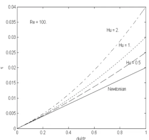
Figure 2 shows the relationship of shearing stress and rate of deformation for a generalized visco-plastic fluid with the dimensionless parameter

L U

H_u =β ₀/µ equals to 0 (Newtonian), 0.5, 1 and 2. The shear thinning characteristics is more significant as the parameter increases.

Programs based upon the above boundary element method have been developed. The MATLAB Version 4.0 is employed as the programming language due to its versatile performance in graphical representation of the computed results. A numerical example is taken as the benchmark to test the accuracy and efficiency of the boundary element solutions. All the programs are executed in an IBM Personal computer.

A problem description of the wall driven Non-Newtonian viscous flow in a cavity is shown in Figure 3. A steady fluid motion is generated by sliding an infinitely long plate lying on top of a cavity. Suppose that all variables are normalized so that the size of cavity is 1×1 and the sliding velocity is 1in the positive x direction. The typical boundary element mesh using 40 elements and 10 x 10 internal cells as well as the element numbering is shown in Figure 4. It is noticed that the boundary conditions of the present problem are all velocities wherein non-zero values are horizontal velocities along the top boundary of the cavity. The velocity vectors, vorticity contour, static pressure contour, streamline contour computed from boundary element method using 40 constant elements and 10 x 10 internal cells are depicted in Figure 5 for Newtonian flows with Re=1 and Figure 6 for

100

Re= , respectively. Totally 19×19=361 internal points are considered to be the sampling points for plotting Figure 5 and 6. All these plots are

in good agreement with the results calculated by Burggraff [39] using finite difference method and Hughes et al. [40] using penalty finite element methods.

Furthermore, Figures. 7 to 10 show the effects of dimensionless parameter H_u on the generalized visco-plastic fluids for Re=1 and Re=100 , respectively. It can be found that the velocity gradients influence the viscous fluids as predicted.

In the current study it is well known that the boundary layer thickness is of the order of Re−1/2and thus at least 10 x 10 internal cells is required for

100

Re= . For Re>120 numerical instability occurs and and it is expected that more fine mesh near walls is required in order to correctly predict the thin viscous layer for moderate Reynolds numbers.

From the boundary element results, Figure 5 and 6, we can observe that at Re=1 the vortex center is located at the centerline of the cavity and then shift in the downstream of the moving plate at Re=100. Vorticity distribution is symmetric at Re=1 due to the vanishing of the convective term. However, when the Reynolds number increases convective term gradually dominate the flow which causes the vorticity stretched and diffused in the cavity. Strong variation of vorticity in the boundary layer is evident along the top and right side of the cavity for Re=100. At

100

Re= a small inviscid core is developed around the vortex center. The growth of the secondary eddies appearing in the bottom corners of the cavity is obvious from the velocity vectors. At Re=100 the eddies at the right hand side of the cavity are grown to about 30% of that at Re=1.

9. Concluding Remar ks

A boundary element method for analysis of steady two-dimensional incompressible Non-Newtonian viscous flow with low Reynolds numbers based on primitive variable is presented. A generalized visco-plastic fluid model is employed to describe the constitutive law for debris flow. The convective terms and terms containing gradient of shear strain rates in the equations of motions are treated as equivalent body forces. The boundary integral equations for velocities and tractions are first formulated and the associated kernel functions for internal velocities, velocity gradients, pressures, vorticities and shearing stresses are explicitly derived. Both domain integration and iterative process are required since nonlinear convective term is present. However, the incompressibility condition is satisfied exactly in the formulation and thus no artificial compressibility and/or penalty are required as in the finite difference and finite element methods. Stream function in the interior is evaluated via the integral equation associated with the Poisson equation. Computational results for the wall driven viscous flow in a square cavity depict that the boundary element method present here provides a convenient tool for

numerical analysis of two-dimensional incompressible viscous flows with low Reynolds numbers. Higher-order elements, multi-grid and/or adaptive grid can be further employed to increase the validity of the scheme for larger Reynolds numbers.

10. ACKNOWLEDGEMENTS

This work is supported by the National Science Council of ROC through grant NSC 90-2211-E151-007. 11. REFERENCES 1. 詹錢登，土石流概論，科技圖書股份有限公司 (2000)。 2. 黃立政，土石流災害防治實務，八十九年教育部 土木工程防災教育改進計劃多媒體教材編撰計 劃，89-土木防災-12 (2001)。

3. Bagnold, R. A., “Experiments on a gravity-free dispersion of large solid spheres in a Newtonian fluid under shear,” Proceedings of Royal Society of

London, Ser. A.,Vol. 225, pp. 49-63 (1954).

4. Takahashi, T., “A mechanism of occurrence of mud-debris flow and their characteristics in motion,” Annuals, Disaster Prevention Res. Inst.,

Tokyo University, No. 20B-2, pp. 405-435 (in

Japanese), (1977).

5. Takahashi, T., “Mechanical characteristics of debris flow,” Journal of Hydraulics Division, ASCE, Vol. 104, No. HY8, pp. 1153-1169 (1978).

6. Chen, C. L., “Generalized visco-plastic modeling of debris flow,” Journal of Hydraulic Engineering,

Vol. 114, No. 3, pp. 237-258(1986).

7. O’Brien, J. S. and Julien, P. Y., “Laboratory analysis of mud flow properties,” Journal of

Hydraulic Engineering, Vol. 114, No. 8, pp.

877-887 (1988).

8. Chen, C.L., Lin, C. H. and Jan, C. D., Rheological model for ring-shear type debris flows,”

Proceedings of the Fifth Federal Interagency

Sedimentation Conference, pp.5:1-5:8 (1991).

9. Julien, P. Y. and Lan, Y., “Rheology of hyperconcentrations,” Journal of Hydraulic

Engineering, Vol. 117, pp. 346-353 (1991).

10. Matsumura, K. and Mizuyama, T. “Experimental study on mechanism of debris flow using light materials,” Shin-Sabo, Vol. 43, No. 1, pp. 16-22 (1990). 11. 游繁結、陳重光， “土石流之基礎研究: (II) 土 石流流速之初步探討”， 中華水土保持學報， Vol. 21, No. 1, pp. 115-141 (1990)。 12. 蘇重光、連惠邦、江永哲， “土石流剖面流速 分佈之研究”，中華水土保持學報，Vol. 24, No. 1, pp. 75-82 (1993)。 13. 何敏龍，土石流發生機制與流動制止結構物之 研究”，國立臺灣大學土木工程研究所博士論文 (1997)。

14. Hassanizadeh, M. and Gray, W. G., “General conservation equations for multiphase systems: 1.

Averaging procedure,” Advances in Water

Resources, Vol. 2, 131-144 (1979).

15. Hassanizadeh, M. and Gray, W. G., “General conservation equations for multiphase systems: 2. Mass, momenta, energy, and entropy equations,”

Advances in Water Resources, Vol. 2, 191-203 (1979).

16 Hassanizadeh, M. and Gray, W. G., “General conservation equations for multiphase systems: 3. Constitutive theory for porous media flow,”

Advances in Water Resources, Vol. 3, 25-40

(1980).

17. Lewis, R. W. and Schrefler, B. A., The Finite Element Method in the Static and Dynamic

Deformation and Consolidation of Porous Media,

Chapter 2, John-Wiley & Sons, Ltd, (1998). 18. Zienkiewicz, O. C., Chan, A. H. C., Chan, Pastor,

M., Schrefler, B. A., and Shiomi, T.,

Computational Geomechanics with Special

Reference to Earthquake Engineering, Chapter 2,

John Wiley & Sons Ltd (1999).

19 . Li, Xi-Kui and Ziekiewicz, O. C., “Multiphase flow in deforming porous media and finite element solutions,” Computers & Structures, Vol. 45, No. 2, pp. 211-227 (1992).

20 .Terzaghi K. von, “The shearing resistance of saturated soils, Proc. 1st ICSMFE, Vol. 1, pp. 54-56 (1936)..

21 . Biot, M. A., “General theory of three-dimensional consolidation,” Journal of Applied Physics, Vol. 12, pp. 155-164 (1941).

22 . Biot, M. A., “General solution of the equation of elasticity and consolidation for a porous material,” Journal of Applied Mechanics, Vol. 23, pp. 91-96 (1956).

23 Fletcher, C. A. J., Computational Techniques for Fluid Dynamics 2, Specific Techniques for

Different Flow Categories, Springer-Verlag,

Heidelberg, 1991.

24 Gresho, P. M., “Some Current CFD Issues Relevant to the Incompressible Navier-Stokes Equations,” Computer Methods in Applied

Mechanics and Engineering, Vol. 87, pp.

201-252, 1991.

25 Anderson, D. A., Tannehill, J. C. and Pletcher, R.

H., Computational Fluid Mechanics and Heat

Transfer, Hemisphere Publishing Corporation,

1984.

26 Carey, G. F. and Oden, J. T., Finite Elements Vol. VI : Fluid Mechanics, Prentice-Hall, Inc., 1986. 27 Reddy. J. N., “Penalty Methods for Finite Element

Approximations of Steady Stokian Flows,”

International Journal of Engineering Science,

Vol. 921, pp. 16-21, 1978.

28 Brebbia, C. A., Telles, J. C. F. and Wrobel, L. C.,

Boundary Element Techniques, Springer-Verlag,

Heidelberg, 1984.

29 Wu, J. C. and Thompson, J. F., “Numerical Solutions of Time-dependent Incompressible

Navier-Stokes Equations Using

Fluids, Vol. 1, pp. 197-215, 1973.

30 Mills, R. D., “Computing Internal Viscous Flow Problems for the Circle by Integral Methods,”

Journal of Fluid Mechanics, Vol. 79, No. 3, pp. 609-624, 1977.

31 Bush, M. B. and Tanner, R. I., “Numerical Solution of Viscous Flow Using Integral Equation Methods,” International Journal of Numerical Methods in Fluids, Vol. 3, pp. 71-92, 1983. 32 Bush, M. B., “Modelling Two-dimensional Flow

Past Arbitrary Cylindrical Bodies Using Boundary Element Formulation,” Applied Mathematical

Modelling, Vol. 7, pp. 386-394, 1983.

33 Onishi, K., Kuroki, T. and Tanaka, M., “An Application of Boundary Element Method to Incompressible Laminar Viscous Flow,”

Engineering Analysis, Vol. 1, No. 3, pp. 122-127,

1984.

34 Dargushi, G. F. and Banerjee, P. K., “A BEM for Steady Incompressible Thermoviscous Fluid Flow,” International Journal of Numerical

Methods in Engineering, Vol. 31, pp. 1605-1626,

1991.

35 Elliot, L., Ingham, D. B. and El Bashir, T. B. A., “Stokes Flow Past Two Circular Cylinders Using A Boundary Element Method,” Computers & Fluids, Vol. 24, No. 7, pp. 787-798, 1995. 36 Zhou, H. and Pozrikidis, C., “Adaptive Singularity

Method for Stokes Flow Past Particles,” journal of Computational Physics, Vol. 117, pp. 79-89, 1995.

37 Pozrikidis, C., Introduction to Theoretical and

Computational Fluid Dynamics, Oxford

University Press, Inc., 1997.

38 Huang, Li-Jeng, “Boundary Element Solutions of Two-dimensional Steady Stokes Flows Based on Primitive Variable Formulation ,” Transactions of the Aeronautical and Astronautical Society of the Republic of China, Vol. 30, No. 4, pp. 261-268, 1998.

39 Burggraf, O. R., “Analytical and Numerical Studies of the Structure of steady Separated Flows,” Journal of Fluid Mechanics, Vol. 24, Pt. 1, pp. 113-151, 1966.

40 Hughes, T. J. R., Liu, W. K. and Brooks, A., “Finite Element Analysis of Incompressible Viscous Flows by the Penalty Function Formulation,” Journal of Computational Physics, Vol. 30, pp. 1-60, 1979.

Figure 1. Typical representative element of multi-phase mixture of debris flow

Figure 2 relationship of shearing stress and rate of deformation for a generalized visco-plastic fluid.

Figure 3 Schematic of wall-driven 2D viscous flow in a square cavity.

Figure 4 Boundary element mesh (40 constant elements and 10 x 10 internal cells) for wall-driven viscous flow in a square cavity.

y

x

u= 0

v= 0

u= 0

v= 0

u= 0, v= 0

u= 1, v= 0

(0,0)

(1,1)

1

10

11

20

21

30

31

40

α

dV

dV

Figure 5 Boundary element solutions for Newtonian Fluid flow (Re = 1): (a) velocity vectors (b) vorticity contour (c) static pressure contour (d) streamline contour.

Figure 6 Boundary element solutions for Newtonian fluid flow (Re = 100): (a) velocity vectors (b) vorticity contour (c) static pressure contour (d) streamline contour.

Figure 7 Boundary element solutions for Non-Newtonian fluid (Re = 1, Hu = 0.0001): (a) velocity vectors (b) vorticity contour (c) static pressure contour (d) streamline contour.

Figure 8 Boundary element solutions for Non-Newtonian fluid (Re = 1, Hu = 0.0002): (a) velocity vectors (b) vorticity contour (c) static pressure contour (d) streamline contour.

Figure 9 Boundary element solutions for Non-Newtonian fluid (Re = 100, Hu = 0.0001): (a) velocity vectors (b) vorticity contour (c) static pressure contour (d) streamline contour.

Figure 10 Boundary element solutions for Non-Newtonian fluid (Re = 100, Hu = 0.0002): (a) velocity vectors (b) vorticity contour (c) static pressure contour (d) streamline contour.