利用空間位移訊號進行結構局部�系統損壞評估

國立台灣大學工程學院土木工程學系 碩士論文

Department of Civil Engineering College of Engineering

National Taiwan University Master Thesis

利用空間位移訊號進行結構局部／系統損壞評估

Application of Spatial Displacement Measurement on Damage Assessment from both Local and Global Structural System

李其航 Chi-Hang Li

指導教授：羅俊雄 教授 Advisor: Chin-Hsiung Loh, Ph.D.

中華民國 101 年 6 月

June, 2012

A

Authorization of Oral Me

i

embers ffor Reseearch Disssertatioon

iii

Acknowledgement

本論文得以順利完整，首先要感謝恩師 羅俊雄教授的細心指導與教誨。承 蒙老師在學業上不厭其煩地提供的建議與幫助，學生在此向羅老師致上由衷的謝 意。另外也感謝 田堯彰教授與 黃震興教授於論文口試期間不吝指正並提供寶 貴建議，使本研究內容在最終能更加充實完整，在此特別致謝。

研究期間，感謝學長趙書賢、盧恭君在研究遇到難題時給予的各項協助。也 感謝同窗陳明徹、陳立豪、杜進國在學習過程中互相扶持與鼓勵。以及學弟曾敏 軒和劉建榮在研究上提供的幫忙。另外在求學期間還有許多值得感謝的人，礙於 篇幅無法一一列舉，但真的發自內心感謝你們。

最後要特別感謝我親愛的家人，多謝你們在背後的支持，使得我能無後顧之 憂地專心求學與研究，僅以本文獻給你們表達我的感謝之意。

v

Abstract (in Chinese)

現今結構物健康監測技術多經由普通接觸式量測計（如：加速度規、速度規…

等）裝設於結構物量取反應訊號進行分析判斷。為獲取結構細部反應資訊而大量 安裝儀器的情況下，此種量測法將會有佈線繁雜以及裝設位置選項過少等問題產 生。然而受惠於光學科技之進步，此問題可有效解決。光學量測方法是將待量測 位置標示上一可經由影像辨識之目標點，藉由攝影裝置觀測目標移動情況進行三 維動態分析。只要目標位於裝置監控範圍內，此方法將能進行大規模位置點計算。

本研究重點在探討此光學量測位移訊號應用於結構系統識別及破壞診斷的適 用性。分析方法分為兩大類。第一類是整體系統識別方法，對於 1.只需結構反應 的斜方差型隨機子空間識別 (Covariance driven Stochastic Subspace Identification, SSI-COV)，和 2.需系統輸入輸出資訊的子空間識別 (Subspace Identification, SI) 作 探討，應用光學多維訊號進行自然頻率與阻尼比分析。再來是研究 3.主成分分析 (Principal component analysis, PCA) 應用此訊號進行結構模態識別。第二類是局部 系統評估，在將光學量測點網格化為數個單元後，應用幾何分析概念進行 4.奇異 譜分析 (Singular spectral analysis, SSA) 獲取單元之主要動態做進一步幾何處理。

另外應用 5.連續小波轉換 (Continuous Wavelet Transform, CWT) 分析訊號不連續 性，對破裂做動時間點進行判斷。單元也可由 6.有限元素法 (Finite element method, FEM) 計算其應變動態行為。本研究將會針對單層雙垮鋼筋混凝土桁架的振動台實 驗進行實際應用。此實驗使用集成式光學量測儀器 DMM (Dynamic Measuring Machine) 量測中間柱三維位移訊號。分析結果顯示應用此種空間位移訊號，整體 系統識別方法可有效的獲取結構物資訊，並對結構變化進行描述；網格化之動態 行為分析也能為結構局部破壞提供重要資訊。

關鍵詞：結構健康監測、空間位移、訊號處理、奇異譜分析、有限元素

vii

Abstract

In this research, the capability of advance spatial displacement measurement for structural health monitoring (SHM) is studied. The method for obtaining this kind of data is different from regular measuring system. It utilizes the optical processing technique to calculate the specific particles’ locations (called targets) within an image.

While taking image and compute the locations over time, the dynamic motion can be estimated. This research employed the three dimensional displacement from optical sensors to identify system and perform damage assessment.

The applied signal analysis methodologies can separate into two categories, global system identification and local element motion detection. For global system, two subspace methods including 1.covariance-driven stochastic subspace identification (SSI-COV) and 2.recursive subspace identification (RSI) are examined. They can obtain the system natural frequency and damping ratio based on different condition. The other method is 3.principal component analysis (PCA), which the system normal modes can be briefly calculated while the measured locations are distributed along the system. For local motion, we can discretize the targets into a set of local elements. These elements motion is detect by 4.singular spectral analysis (SSA), 5.continuous wavelet transform (CWT), and 6.finite element method (FEM). The extracted information is used to

viii

describe the structural local properties and detect the damage occurrence. To examine the applications of these methodologies on real three dimensional displacement data, a shake table test of one-story two-bay RC frame performed in the NCREE is selected.

This experiment installed a totally integrated optical measuring system (DMM, by NDI Inc.) on its central column to obtain the displacement. The analysis results show that this kind of data is capable for system identification, and the detection of damage is also feasible. Detail analyzes the discrete elements. The damage location may be obtained.

Keywords: Structural Health monitoring, spatial displacement, signal processing,

singular spectral analysis, finite element method

ix

Contents

Authorization of Oral Members for Research Dissertation ... i

Acknowledgement ... iii

Abstract (in Chinese) ... v

Abstract ... vii

Contents ... ix

Table List ... xii

Figure List ... xiii

Chapter 1. Introduction ... 1

1.1 Motivation ... 1

1.2 Literature Review ... 2

1.3 Research Objective ... 4

Chapter 2. Signal Analysis Methodology ... 7

2.1 Introduction ... 7

2.2 Global System Characteristics Identification ... 7

2.2.1 Covariance-Driven Stochastic Subspace Identification (SSI-COV) ... 8

2.2.2 Recursive Subspace Identification (RSI) ... 12

x

2.2.3 Principal Component Analysis (PCA) ... 16

2.3 Local Element Motion Analysis ... 19

2.3.1 Singular Spectral Analysis (SSA) ... 20

2.3.2 Continuous Wavelet Transform (CWT) ... 23

2.3.3 Finite Element Method (FEM) ... 25

2.4 Chapter Summary ... 29

Chapter 3. Experimental Survey ... 33

3.1 Description of the Experiment ... 33

3.2 Preview of System Physical Properties ... 35

3.3 Optical Data Preprocessing ... 36

3.3.1 Three Dimensional Affine Transformation ... 36

3.3.2 Shifting of Target Positions ... 38

3.4 Global System Characteristics Identification ... 39

3.4.1 Global System Identification by SSI-COV ... 39

3.4.2 Global System Identification by RSI ... 41

3.4.3 Effective Mode Shape by PCA ... 43

3.4.4 Vector Space Damage Indicator by SSI-COV ... 44

3.5 Local Element Motion Analysis ... 47

xi

3.5.1 Local element principal motion by SSA... 47

3.5.2 Displacement non-continuity by CWT ... 51

3.5.3 Local element strain by FEM ... 52

3.5.4 Connection between Local Analysis Methodologies... 54

3.6 Chapter Summary ... 55

Chapter 4. Conclusions ... 61

4.1 Research Conclusions ... 61

4.2 Recommendations for Future Work ... 65

References ... 66

xii

Table List

Table 3-1 Physical parameters of shake table test (Freq. refer to Mao) ... 71

Table 3-2 White noise analysis result by SSI-COV ( = 0.9) ... 71

Table 3-3 Seismic analysis result by RSI and PCA ... 72

Table 3-4 Element with oscillation principal motion by SSA ... 72

xiii

Figure List

Figure 2-1 Flowchart of SSI-COV algorithm ... 73

Figure 2-2 Scheme of on-line recursive identification ... 73

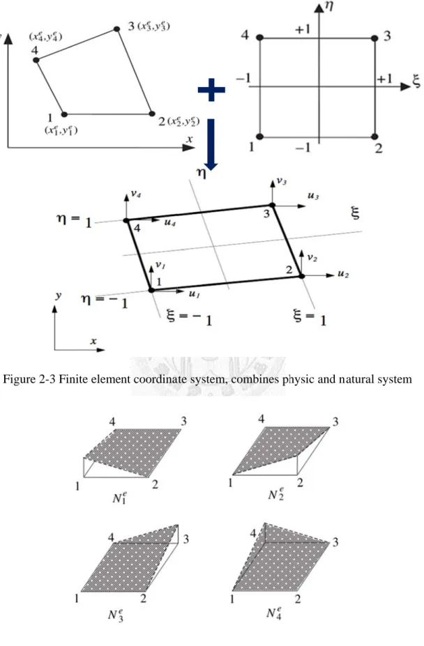
Figure 2-3 Finite element coordinate system, combines physic and natural system ... 74

Figure 2-4 Scheme of Q4 element shape function ... 74

Figure 2-5 Strain definition of unit element ... 75

Figure 2-6 Research framework ... 75

Figure 3-1 Specimen of one-story two-bay RC frame ... 76

Figure 3-2 Design detail of elements and specimen diemnsion ... 76

Figure 3-3 Configuration of general measuring system ... 77

Figure 3-4 Configuration of optical measuring system ... 77

Figure 3-5 Optical sensing system in the shake table test ... 78

Figure 3-6 Normalized input ground motion of TCU082 ... 78

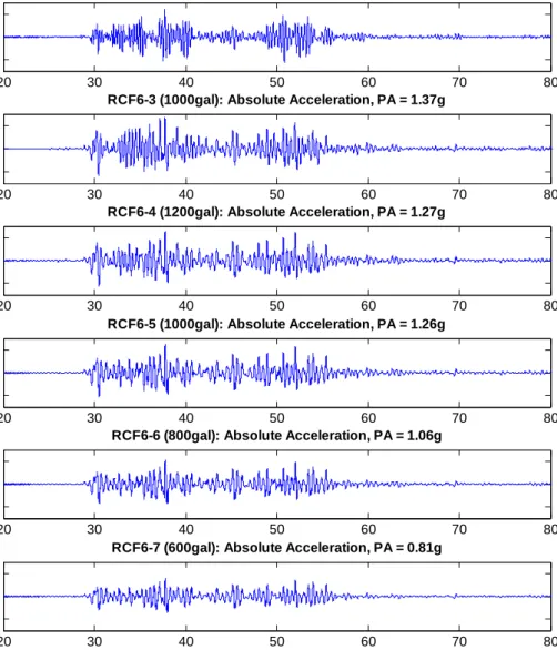
Figure 3-7 Absolute acceleration response of the series of excitations ... 79

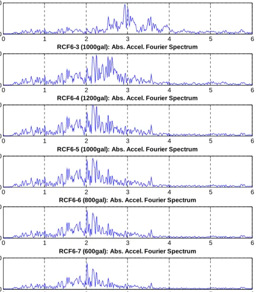
Figure 3-8 Absolute acceleration Fourier spectrum of the series of excitations ... 80

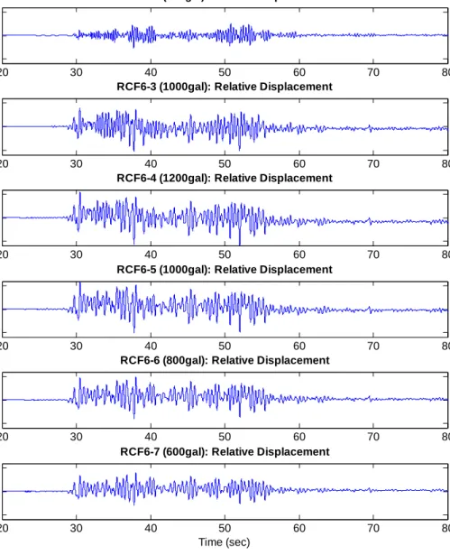
Figure 3-9 Relative displacement of the series of exciations ... 81

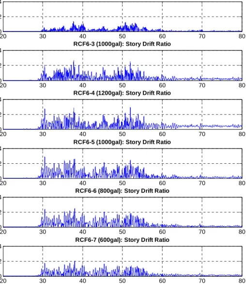
Figure 3-10 Inter story drift ratio of the series of excitations ... 82

xiv

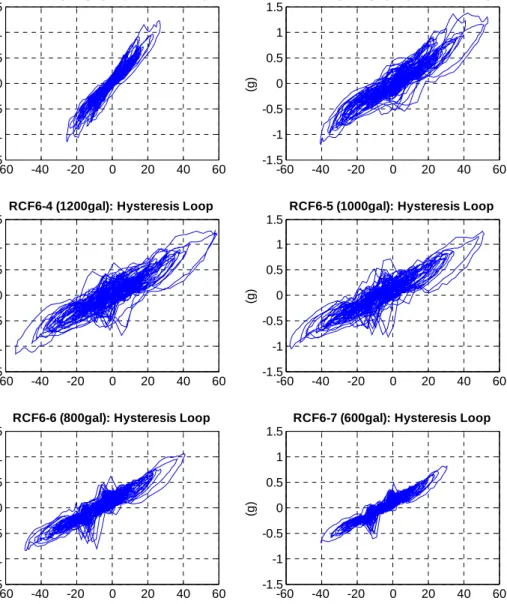
Figure 3-11 Hysteresis behavior of the series of excitations ... 83

Figure 3-12 DMM of NDI Inc.: (a) Optical tracker and (b) targets. ... 84

Figure 3-13 Scheme of two different coordinate systems ... 84

Figure 3-14 System natural frequency stability diagram, = 0.7 ... 85

Figure 3-15 System natural frequency stability diagram, = 0.8 ... 86

Figure 3-16 System natrual frequency stability diagram, = 0.9 ... 87

Figure 3-17 Scheme of space difference (a) reference, (b) current, and (c) compare .... 88

Figure 3-18 Damage indicators of space projection ... 88

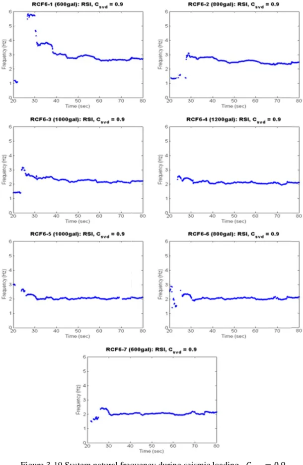
Figure 3-19 System natural frequency during seismic loading, = 0.7 ... 89

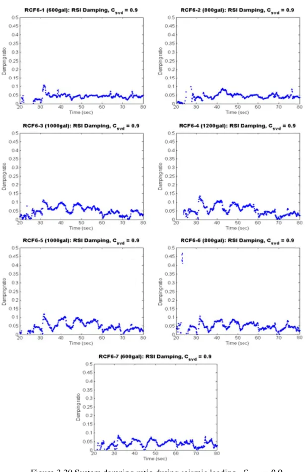
Figure 3-20 System damping ratio during seismic loading, = 0.7 ... 90

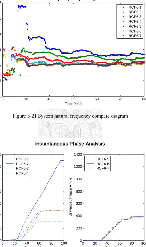
Figure 3-21 System natural frequency compare diagram ... 91

Figure 3-22 Instantaneous phase analysis ... 91

Figure 3-23 Effective mode shape (a) ... 92

Figure 3-24 Effective mode shape (b) ... 92

Figure 3-25 Effective mode shape (c) ... 93

Figure 3-26 Effective mode shape (d) ... 93

Figure 3-27 Variation of modal contribution ... 94

Figure 3-28 Mesh grids of optical sensors on central column ... 94

xv

Figure 3-29 Nodal order for a particular element ... 95

Figure 3-30 Scheme of damage detection: (a) vertical, (b) laterial difference, and (c) y direction bending analysis ... 95

Figure 3-31 RCF6-1 X Dir. element four nodes principal motion ... 96

Figure 3-32 RCF6-1 Y Dir. element four nodes principal motion ... 97

Figure 3-33 RCF6-1 X Dir. unrecoverable element principal motion ... 98

Figure 3-34 RCF6-1 Y Dir. unrecoverable element principal motion ... 99

Figure 3-35 RCF6-4 X Dir. element four nodes principal motion ... 100

Figure 3-36 RCF6-4 Y Dir. element four nodes principal motion ... 101

Figure 3-37 RCF6-4 X Dir. unrecoverable element principal motion ... 102

Figure 3-38 RCF6-4 Y Dir. unrecoverable element principal motion ... 103

Figure 3-39 RCF6-1 X Dir. square -sum of unrecoverable signals ... 104

Figure 3-40 RCF6-1 Y Dir. square-sum of unrecoverable signals ... 104

Figure 3-41 RCF6-2 X Dir. square-sum of unrecoverable signals ... 105

Figure 3-42 RCF6-2 Y Dir. square-sum of unrecoverable signals ... 105

Figure 3-43 RCF6-3 X Dir. square-sum of unrecoverable signals ... 106

Figure 3-44 RCF6-3 Y Dir. square-sum of unrecoverable signals ... 106

Figure 3-45 RCF6-4 X Dir. square-sum of unrecoverable signals ... 107

xvi

Figure 3-46 RCF6-4 Y Dir. square-sum of unrecoverable signals ... 107

Figure 3-47 RCF6-5 X Dir. square-sum of unrecoverable signals ... 108

Figure 3-48 RCF6-5 Y Dir. square-sum of unrecoverable signals ... 108

Figure 3-49 RCF6-6 X Dir. square-sum of unrecoverable signals ... 109

Figure 3-50 RCF6-6 Y Dir. square-sum of unrecoverable signals ... 109

Figure 3-51 RCF6-7 X Dir. square-sum of unrecoverable signals ... 110

Figure 3-52 RCF6-7 Y Dir. square-sum of unrecoverable signals ... 110

Figure 3-53 Element B2 Y Direction bending angle analysis ... 111

Figure 3-54 RCF6-1 CWT analysis of element B2 lef edge difference ... 112

Figure 3-55 RCF6-1 CWT analysis of element B2 right edge difference ... 112

Figure 3-56 RCF6-2 CWT analysis of element B2 lef edge difference ... 113

Figure 3-57 RCF6-2 CWT analysis of element B2 right edge difference ... 113

Figure 3-58 RCF6-3 CWT analysis of element B2 lef edge difference ... 114

Figure 3-59 RCF6-3 CWT analysis of element B2 right edge difference ... 114

Figure 3-60 RCF6-4 CWT analysis of element B2 lef edge difference ... 115

Figure 3-61 RCF6-4 CWT analysis of element B2 right edge difference ... 115

Figure 3-62 RCF6-5 CWT analysis of element B2 lef edge difference ... 116

Figure 3-63 RCF6-5 CWT analysis of element B2 right edge difference ... 116

xvii

Figure 3-64 RCF6-6 CWT analysis of element B2 lef edge difference ... 117

Figure 3-65 RCF6-6 CWT analysis of element B2 right edge difference ... 117

Figure 3-66 RCF6-7 CWT analysis of element B2 lef edge difference ... 118

Figure 3-67 RCF6-7 CWT analysis of element B2 right edge difference ... 118

Figure 3-68 Strain field variation from RCF6-1 to RCF6-7, ... 119

Figure 3-69 Strain field variation from RCF6-1 to RCF6-7, ... 120

Figure 3-70 Strain field variation from RCF6-1 to RCF6-7, ... 121

Figure 3-71 RCF6-4 Strain field trend of ... 122

Figure 3-72 RCF6-4 Strain field trend of ... 123

Figure 3-73 RCF6-4 Strain field trend of ... 124

Figure 3-74 Normal strain tendency approach by principal motion ... 125

Figure 3-75 Normal strain tendency approach by principal motion ... 126

Figure 3-76 Shear strain tendency approach by principal motion ... 127

Figure 3-77 Local analysis result comparison (a) ... 128

Figure 3-78 Local analysis result comparison (b) ... 129

Figure 3-79 Local analysis result comparison (c) ... 130

Figure 3-80 Local analysis result comparison (d) ... 131

1

Chapter 1. Introduction

1.1 Motivation

Structure health monitoring (SHM) has become more and more important in the civil engineering structure. Since the structures are deteriorated under service condition, it is recommended observing the structure health over time. The structure dynamic response measurement is very useful information. These measured signals contain the system response properties. Base on signal processing techniques, one can extract the signal feature for structure health monitoring and damage assessment.

The vibration-based SHM framework not only relies on the signal processing techniques but also the sensor arrangement. The recent structure measuring system utilizes normal contact sensors, for example accelerometers, placed on specific locations to represent the structure DOFs. These locations are mostly selected the floor slabs according to structural analysis concept. But if we want a more detail information within the floors, these sensors are not suitable because of installation difficulty. A measuring technique on this kind of location is needed. We discover that a novel technique utilized the optical processing method can measure particles’ motions within an image over time with a reliability accuracy. This optical measuring technique can

2

implement on the locations that the normal contact sensors are difficult to install.

Therefore, we can extract both global and local information from the structure by combining the optical and normal contact sensors.

These optical sensors are distributed within a region of local structure. The research on the application of presents signal processing techniques is needed. It is believed that the measured information can be used to identify the system and perform local damage assessment for structure health monitoring.

1.2 Literature Review

There have already lots of researches of signal processing methodologies on damage detection and system identification. Science the optical measuring system measures a large amount of sensor locations over time, methodologies with multivariate techniques are more suggested in this research.

For system identification, the subspace identification method is proved that its capability to observe the structure characteristics [15, 26]. With recursive updating the measurement data, an on-line system monitoring is obtained. Moreover, the method relies on the singular value decomposition (SVD). Since the system information is contained in the singular vectors of SVD, damage assessment can achieve by observing

3

the vector space expanded by singular vectors. There are researches utilize the space projection theorem to detect damage according to the change point of dataset [17, 23].

The principal component analysis (PCA) is another signal feature extraction technique. It is one of the well-known methods for multivariate analysis. Originally, the PCA are used to perform data compression [18]. Feeny [7] conducted the applicability of structural dynamic response with PCA to real experiment test. It is proved that PCA has the ability to express the structural normal modes under some condition [3]. While the sensors are arrange into an array form, the PCA can be applied on the data to detect the damage location [5]. The advantage is that the PCA is straight forward and has capability for nonlinear applications.

The singular spectral analysis (SSA) can extract not only features of one signal but also mutual features of signals with multivariate. It has been proved that it can decompose the data into trend, harmonic wave, and noise term [24]. The SSA has a widely application. In the civil engineering scope, there are studies on the analysis of seismic response data [11, 21] to grab site vibration information. The concept of SSA is relative to PCA. It is like analysis the signal with the embedding theorem [20] using PCA. And the decomposed results are the signal principal feature that can represent the original signal.

4

The analysis methods mentioned above are capable for multivariate data analysis.

But they are still some processes need to study for the real application on damage assessment with the array of optical sensors. The explanation is in remaining chapters.

1.3 Research Objective

The objective of this research is to conduct a survey on the applications of the spatial displacement data and provides to a series of shake table test of the RC frame to check the capability. The displacement data measure the structure three dimensional motions over time with large amount of the sensing locations. It is expected that one can perform the system identification and detect the damage using this detail spatial displacement information.

The organization of this research is briefly described as follows:

Chapter 1: Describe the research motivation and literature review of some present

system identification and damage assessment techniques.

Chapter 2: Introduce the signal processing methodologies used in this research. The

introduced methodologies can perform system identification and feature extraction on the spatial displacement data.

5

Chapter 3: Perform the methods on the seismic response of a one-story two-bay RC

frame. The analysis is separated into two categories: global system identification and local motion detection. The selected parameters and results of each method are discussed. Finally, the analysis results will be

compared to each other.

Chapter 4: Summaries for the use of the proposed techniques are listed in this

chapter, and the potential research topics are indicated at the end.

7

Chapter 2. Signal Analysis Methodology

2.1 Introduction

In this chapter, the algorithm of signal analysis methodologies used in this research will be introduced. These methodologies are separated into two categories according to their application, which are global system characteristics identification and local element motion analysis. After introduction, all of the analysis methodologies will be applied on the spatial displacement signals acquired from the experiment mentioned in the next chapter to identify the system parameters and detect the damage occurrence.

2.2 Global System Characteristics Identification

Nowadays, there are several signal processing techniques can perform global system characteristics identification. These methods can be categorized into parametric and non-parametric methods, or model based and non-model based. To choose reliable methods for this study, there are three different methods are selected. Two of them are subspace methods (SSI-COV and RSI) based on the discrete time state space model and can identify system natural properties including frequency, damping, and mode shape.

The other is principal component analysis (PCA) which is a time series decomposition

8

technique that can briefly obtain the system normal modes. Detail introductions of these methodologies are mentioned in the following sections.

2.2.1 Covariance-Driven Stochastic Subspace Identification (SSI-COV)

The SSI-COV algorithm is an expansion of the stochastic subspace identification (SSI) technique which identifies stochastic state space model using output only data.

Instead of the original SSI algorithm [22, 26], the SSI-COV calculates the system via assemble of block covariance matrices. Since these SSI algorithms based on concepts from linear algebra, state space model, and statistics, they have been proven to perform on the structure identification [15, 28]. Only one restrict of the SSI based algorithms is the output measurement should be ambient response of structure because of the assumption of noise input. The derivation of SSI-COV is as follows:

Stochastic Discrete Time State Space Model

For a system motion equation

Mx Cx Kx F Lu  ₊  _{+ = =}

, where M ,

C

, and

n n×

∈

K 

are system mass, damping and stiffness matrix;

x

∈



^n×1 and

u  _∈

^m×1 are displacement and input force vector;

n

and

m

represent number of DOFs and number of inputs. The state space equation is written as

( ) ^t

^{= c}

( ) ^t

^{+ c}

( ) ^t

^,

X



A X B u

(2.1)

9

2 2 2

1 ⁿ1 ^{n n}, and 1 ^{n m},

c c

× ×

− − −

 

=− ∈

 

=− ∈

 − 

0 I

A B 0

M K M C ^ M L ^

(2.2)

where

X ( ) ^t

^=

x

^T

( ) ^t x 

^T

( ) ^t

^^T∈



^2n×1 is the state vector at continuous time t and

( )

c

t

A

,

^B

^c

( ) ^t

are continuous time state matrix and input matrix. If there are only

l

DOFs has been measured, and the measurement response can be acceleration, velocity or displacement. The output observation vector

^y ( ) ^t

^∈

 can be written as

^l×1

( ) ^t

^{= a}

( ) ^t

^{+ v}

( ) ^t

^{+ d}

( ) ^t

y C



x C x



C x

, where

C

_a,

C

_v, and

C

_d∈

 are output location

^{l n×}

matrices. To transform

^y ( ) ^t

into state space representation, it becomes

( ) ^t

^{= c}

^X ( ) ^t

^{+ c}

( ) ^t

^,

y C D u

(2.3)

1 1 2 1

, and .

l n l m

c d a v a c a

− − × − ×

= − − ∈ = ∈

C C C M K C C M C  D C M L 

(2.4)

This equation is called observation equation. The

C

_c is output matrix and

D

_c is direct transmission matrix. Since all data are measured in discrete time, Eq.(2.1) and Eq.(2.3)

need to be transformed into discrete time state space model, that is

1 ,

,

k d k d k k

k c k c k k

+ +

+

= +

= +

X w

y

A X B u

X u v

C D

(2.5)

with the

A

_d =

e

^AcΔt,

^B

^{d =}

( ^A

^{d −I}

) ^{A B}

^{c−1 c, and}

^X

^{k =}

^X ( ) ^{k t}

^Δ . The terms

w

_k and

v

_k at the end of equations are the error from noise and measurement. If the input force satisfies the stochastic expression, the discrete time state space mode can be further transformed into

1

,

.

s s s

k d k k

s s s

k c k k

+

=

=

+ +

X w

y X v

A X

C

(2.6)

10

This equation is called stochastic state space model. The SSI-COV identifies the system matrices (

A

_d and

C

_c) of Eq.(2.6) only using the output measurement

y .

^s_k

Hankel Covariance Matrix of SSI-COV

Assume the output measurement

^y ( ) ^t

^is

[ ^y

¹

^y

^{2 }

^y

^N

]

, the first step of the SSI-COV is to gather the measurement vectors into a data Hankel matrix that is

1 2

2 3 1

1 1

1 2

2 3 1

2 2 1

,

s s s

j

s s s

j

s s s

p i i i j

s s s

i i i j

f

s s s

i i i j

s s s

i i N

+

+ + −

+ + +

+ + + +

+

 

 

 

 

 

  = 

   

 

   

 

 

 

 

 

y y y

y y y

Y y y y

y y y

Y

y y y

y y y





   







   



(2.7)

where

Y

_p∈



^{li j×} denotes the past measurements and

Y

_f ∈



^{li j×} is the future measurements. After this, the block Toeplitz matrix is obtained by

1 1

1 2

2 1 2 2

1 .

i i

i i

i i

T f p

i

N

− +

− −

 

 

 

=   =

 

 

R R R

R R R

T Y

R R

Y R





   



(2.8)

Each

R

_i defines an output covariance between two time instant with lag i .

Extended Observability Matrix and Singular Value Decomposition

According to the derivation based on stochastic properties [15], the block Toeplitz matrix T can be decomposed into the multiplication of the extended observability

11

matrix

O

_i∈



^li×2n and the reversed extended stochastic controllability matrix

2n li i

∈ ×

Γ 

as follows

1

1 i ,

i i

i

−

−

 

 

   

= =  

 

 

C

T O Γ CA A G A G G

CA

 

(2.9)

where the i here denotes the order of the Toeplitz matrix T . The singular value decomposition (SVD) is utilized to perform this factorization. Representation of SVD is

[

^{1 2}

]

^{1 1 1 1 1}

2 2

,

T

T T

T

 

 

= =     ≅

   

S 0 V

T USV U U S

S U V

0 V

(2.10)

where

U  _∈

^{li li×} and

V _∈ 

^{li li×} are the orthogonormal matrices, and

S

is the diagonal singular values. To perform data compression from

USV

^T to

U S V , the

_{1 1 1}^T

C

svd defined the percentage of preservation is determined. Assume the diagonal terms of

S

are

[ ^s

¹

^s

^{2 }

^s

^li

]

^{. Size}

^N

^of

^S

¹ is the minimum even number satisfied

( )

1

trace .

i sv

i

d N

s C

=

≥ ×

 ^S

^(2.11)

After the data compression, we can compare the form between Eq.(2.9) and Eq.(2.10).

The extended observability matrix

O

_i can be defined as

1 2 1 1 .

i = S

O U

(2.12)

State Matrix and System Properties

The system matrices

A

_d and

C

_c can be easily extracted from

O

_i. We can compare to Eq.(2.9) for the elements of matrix

O

_i, the system matrices are

12

( )

( ( ) ) ^{( )}

1: ,: ,

1: 1 ,: 1 : ,: ,

c i

d i i

l

l i

⁺

l li

= − +

= C O

A O O

(2.13)

where

( )

⋅ denotes pseudo inverse. As soon as the discrete state matrix ⁺

A

d is derived, we can transform it into the continuous form

A

_c following the relation in

Eq.(2.5) and apply eigen-decomposition of it that

1

,

.

c m

c m

c c

=

−

=

=

A Λ Ψ A Ψ

C C Ψ

(2.14)

The superscript

m

denotes the matrices in modal coordinate. Each eigenvalue

λ

_k ⁱⁿ

Λ is a complex number and has its conjugate value λ

_k^′. After eigenvalues are

determined, the system natural frequency

f

_k and damping ratio

ξ

_k can be solved as

( )

²

( )

^{2 Re}

( )

1 Re Im , and .

2 2

k

k k k k

k

f f

λ λ ξ λ

π π

+ =−

= (2.15)

Derivation from Eq.(2.7) to Eq.(2.15) represents the SSI-COV algorithm of system identification. Flowchart of the SSI-COV algorithm can be concluded as Figure 2-1.

2.2.2 Recursive Subspace Identification (RSI)

Different from the SSI-COV based on the noise property of input data, the subspace identification (SI) method utilizes both input and output signals to perform the system identification [26]. This makes the identified system properties more reliable while the measurements are not satisfying the ambient condition. Moreover if the

13

system varies over time, the SI algorithm should analysis with a moving window to perform on-line system identification (Figure 2-2). To speed up the repeating calculation of the SI, a recursive algorithm that solves equation based on the previous information is needed. This section will explain the algorithm of the SI technique first, and then introduce the recursive algorithm of LQ factorization briefly. The procedures of the recursive-SI (RSI) are as follows:

Hankel Matrices of Subspace Identification

The origin of the SI algorithm is based on state space model shown in Eq.(2.5).

Since we already defined an output data Hankel matrix Eq.(2.7) at the SSI-COV algorithm, the input data

^u ( ) ^t

can also be arrange in the Hankel form that is

1 2

2 3 1

1 1

1

2

2

2 3 1

2 1

,

j

j

p i i i j

i i i j

f

i i i j

i i N

+

+ + −

+ + +

+ + + +

+

 

 

 

 

 

   = 

   

 

   

 

 

 

 

 

u u u

u u u

U u u u

u u u

U

u u u

u u u





   







   



(2.16)

where

U

_p∈



^{mi j×} denotes the past input measurements and

U

_f ∈



^{mi j×} is the future input measurements. Furthermore, the special Hankel matrix can be defined as

(^{m l i})

.

p j

p p

 

+ ×

=   ∈

  Ξ U

Y 

(2.17)

14

Extended Observability Matrix and LQ Factorization

For system characteristics identification, the extended observability matrix

O

_i is needed. The SI algorithm utilizes both oblique projection theorem and the MOESP theorem [25] of LQ factorization to extract the matrix

O

_i. The procedures are

1,1 1,1

2,1 2,2 2,1

3,1 3,2 3,3 3,1

,

T f

T p

T f

    

    

 =  

     

 

U L 0 0 Q

L L 0 Q

L L L Q

Y

Ξ

(2.18)

( ^Y

^{f Uf}

^Ξ

^p

) ^U

^f⊥

^{= O X U}

ⁱ

^

^{i f⊥}

^{= L Q}

^{3,2 2,1T}

^,

^(2.19)

( )

^3,2

^{( )}

column space

L

=column space

O

_i . (2.20) where ⋅ ⋅ and ^⊥

⋅

_⋅ are orthogonal projection and oblique projection operator;

Eq.(2.18) is LQ factorization and Eq.(2.19) is oblique projection of Hankel matrices.

According to derivation [27], the relation between the oblique projection and the LQ factorization is defined and they can connect with the extended observability matrix

O

_i in Eq.(2.19). Following this equation, only

L of LQ factorization is needed for

_3,2

system identification. Furthermore, column space of it can obtained from SVD, that is

[ ]

^{1 1}

3,2 1 2 1 1 1

2 2

1

, .

T

T T

T

i

 

 

= =   ≅

  

=



S 0 V

L USV U U U

0 S O

S V U

V

(2.21)

In this equation, the

C

_svd defines in Eq.(2.11) is also introduced to denoise the SVD result.

15

State Matrix and System Properties

After the system extended observability matrix

O

_i is obtained, the same procedures introduced in the SSI-COV algorithm from Eq.(2.13) to Eq.(2.15) can be applied to obtain the system natural properties. Besides, another parameter

C

_omac is taken to filter out the noise modes. The idea is based on the matrix

O

_i can be reconstructed from two different approaches. First is direct calculation that

( )

[

^{1 2}

]

1

.

m c

m m

c c

m

i N

m m i

c c

−

 

 

 

=   =

 

 

 

φ C

C A

C

φ O

A

φ

 

(2.22)

The other is based on the idea of data composition of Eq.(2.12), that is

[ ]

1 1 2 .

m

i =

O Ψ

i =

U Ψ

=

φ φ φ

N

O     

(2.23)

Therefore, the coherence between the vectors

φ

_i and

φ

_i are defined as

( ) ( ) ( )

*

* *

, for 1 . OMAC

T

i i

i T T

i i i i

i N

=

φ φ

=

φ φ φ φ





 

(2.24)

The larger

OMAC

_i value reflects the higher correlation. It means the identification of

i -th mode will be more reliable. Therefore the criterion is set as

OMAC

_i

≥ C

_omac

.

^(2.25)

Based on Eq.(2.25), we can just preserve the modes satisfied this condition and employ these remaining modes for system identification through Eq.(2.15).

16

Given Rotation of Recursive SI

To identify system on-line and keep a fast calculation speed, a recursive algorithm is needed. The recursive-SI algorithm can be separated into following three parts:

1. Calculate the SI for the initial round and keep the LQ factorization result.

2. For the following cases, the Hankel matrix in Eq.(2.18) should be updated with new measurement and eliminate the old data with the same size.

3. The LQ factorization of the new Hankel matrix can be replaced by applying a recursive algorithm, named given rotation, two times on the previous LQ result for updating and eliminating the data.

Thus, the calculation of LQ factorization of the whole new Hankel matrix is omitted. It will not only save lots of computation time but also preserve the accuracy. Detail introduction of the processes of RSI algorithm can refer to [26, 27].

2.2.3 Principal Component Analysis (PCA)

The PCA also known as Karhunen–Loève transform is first introduced by Pearson [18] as a line fitting algorithm in data space. The concept of PCA is to find orthogonal bases called principal components (PCs) which represented the largest possible variance direction of the data. Moreover, the PCs are arranged in descending order which means

17

the first PC has largest data variance. For dynamic analysis, PCs can represent system normal modes based on few assumptions. Therefore, it is also called proper orthogonal decomposition (POD) and the extracted PCs are called proper orthogonal modes (POMs). The procedures of PCA algorithm for structural analysis are as follows:

Data Ensemble Matrix and Correlation Representation

The PCA starts from the construction of the ensemble data matrix X of all measured response signals, that is

( ) ( ) ( )

( ) ( ) ( )

( ) ( ) ( )

1 2 1

2 1 2

1 2

1 1

2 2

,

N

N

m m m N

x t x t x t

x t x t x t

x t x t x t

 

 

 

=  

 

 

 

X





   



(2.26)

each

x

_i represents a time series measurement of acceleration, velocity, or displacement on a particular position of the structure. The suffix

m

means total number of measurement. After the ensemble matrix X is arranged, the covariance matrix

m n×

∈

C 

can be derived as

1

^T

.

= N

C XX

(2.27)

Orthogonal basis of Principal Components

Based on the derivation [13], the orthogonal basis of PCs can be derived from the eigen-decomposition of matrix

C

that is

1

,

=

−

C ΨΛΨ

(2.28)

18

where the eigenvectors Ψ are the PCs of matrix X .

Normal Modes and Principal Components

Assume ensemble matrix X of structural response satisfies modal combination theorem. Therefore, X could be written as the combination of normal modes that

1

T T,

i i m

i=

=

^ΦQ

=

 ^{φ q}

X

(2.29)

where the

φ

_i,

q

_i, and

m

are normal modes, general coordinates, and number of modes can be extracted. Assume the structural mass matrix is homogeneous that

= m

M I

and satisfies

φ Mφ

^T_{i j} =

δ

_ij. Combine Eq.(2.27) and Eq.(2.29) together with

right multiple

φ

_i, it will become

1 1 1

1 1

T T

.

m m

T kk

k i i j

m

i j i

j k i i k

N N m

δ

= = =

=  = 

C φ φ q q φ φ φ q q

(2.30)

Furthermore, assume the damping ratio is relatively small. Eq.(2.30) can be rewritten as

lim 0, for

1 .

lim 0, for

T i k

T kk

k k k k

N

T k N

i

i k N

N m

i k N

δ

→∞

→∞

 = =

 →

  ≠ =



= q

φ φ

q q

C q q

q

(2.31)

In this equation,

¹

^T_{k k} ^kk

N m

q q

δ is constant and can be assumed as

λ

_k. Therefore, we get

k

= λ

k k

.

Cφ φ

(2.32)

Eq.(2.32) is equivalent to Eq.(2.28) as eigen-decomposition of matrix

C

. Thus, we have proven that PCs Ψ are the same as structural normal modes Φ .

19

Through the derivation [3], three conditions need to be guaranteed for the equivalent of normal modes. There are 1.the structural damping ratio is small in all cases, 2.number of observation is large enough, and 3.the mass distribution is homogenous. If the mass are not uniform distribution, a modified correlation matrix is suggested [10] to improve the analysis result, that is

1

^T

.

m

= N XX M

C

(2.33)

The mass matrix M should be determined first to do the modification. According to numerical survey [2], PCA though may lose some precision; it can obtain the structural normal modes very briefly.

2.3 Local Element Motion Analysis

Since the spatial displacement data can represent an object motion very detail, there must have some local information according to the mesh elements of these sensors.

To get the information from elements’ three dimensional motion, the singular spectral analysis (SSA) as powerful multivariate signal decomposition technique is introduced.

Moreover, the signal discontinuity is detected by continuous wavelet transform (CWT) to find the crack effect. Finally, finite element method (FEM) which is well defined in mesh filed will also be discussed.

20

2.3.1 Singular Spectral Analysis (SSA)

The SSA as a linear time series feature extraction technique is similar to apply the PCA on the time series with the embedding theorem [24] which combines lagged copies of the original data from lag 1 to k time steps. By performing the SSA, time series will be decomposed into several feature components that can be treat as trend, oscillation, or noise components [6, 9]. The procedures of SSA can be separated into four steps, which are (1) embedding, (2) SVD, (3) grouping, and (4) reconstruction. Details introduction are described as follows:

Embedding Theorem

Consider a time series

^y ( ) ^t

⁼

[ ^y

⁰

^y

^{1 }

^y

^N−1

]

of length

N

. The embedding theorem maps the time series into a sequence of multi-dimensional lagged vectors. In this step, the only SSA parameter L called window length should be determined, where the range is

2 ≤ ≤ L N 2

. Then

K = − + N L 1

lagged vectors are embedded to form the trajectory matrix X ,

( ) ^{[ ]}

0 1 2 1

1 2 3

,

, , 1 2 3 4 1 1 2

1 1 1

,

K

K L K

i j i j K K

L L L N L K

y y y y

y y y y

x y y y y

y y y y

−

= +

− + − ×

 

 

 

 

= =

 

 

 

=

 

X x x x





 

    



(2.34)

21

where

^x

^{i =}

[ ^y

ⁱ⁻¹

^y

^{i }

^y

^{i L+ −2}

]

^{T for}

^{1 ≤ ≤ i K}

is the i -th lagged vector. One of the properties of trajectory matrix is that it is Hankel matrix which the skew diagonal terms (

i

+ =

j

const.) are equal. If the analysis data are multivariate, each component of

^{y t} ( )

should be treated as a vector form that

^y

^{i }

{ } y

ⁱ = ^

^y

^1,i

^y

^2,i

 ^y

^{n i, }^T where

n

is the total number of variate.

Singular Value Decomposition (SVD)

The second step is to perform SVD to the trajectory matrix X . First define a matrix

S ₌ XX

^T . The eigenvalues of matrix

S

are denoted by

λ

₁

, ^ , λ

_n ^{in the} descending order (

λ

₁

≥ ≥ ≥  λ

_n

0

) and the corresponding eigenvectors are

u

₁

,  , u

_L. Then, define vector

v

_i = X^T

u

_i

λ

_i . The SVD of the trajectory matrix X can be written as

1 2

1

.

d

i

T

i i i d

λ

=

= +

=

 ^{u X}

+

^X

+

X v



X

(2.35)

Each

X

_i =

λ

_i

u v

_i ^T_i is a rank 1 elementary matrix and

d

is max i with

( ) λ

_i

> 0

^. The set of

λ

_i is called singular values (SVs). It contains the important information of decomposition quality and should be plotting out as singular spectrum.

Grouping

After the SVD is applied, the trajectory matrix X has been decomposed into several components. The grouping step is to select the appropriate elementary matrices

22

to form an approximate trajectory matrix X

^

. Decision-making of which components should be selected can refer to the singular spectrum. The singular spectrum shows brief decomposed properties [6] that oscillation comes with two closed SVs in a pair; trend component has a lonely SV in a certain amount; series of low value SVs may represent signal noise. Therefore through singular spectrum, one can group correlative eigentriples (

λ

_i

u v ) following the type of components would like to reconstruct.

_i ^T_i

Reconstruction (Diagonal Averaging)

Since approximate trajectory matrix X

^

is no longer kept the property that skew diagonal terms are equal, new time series

^y ( ) ^t

should be reconstructed by diagonal averaging the matrix X

^

based on this property. The scheme of diagonal averaging is shown as

( ) ( )

1,1 1,2 1,3 1,

2,1 2,2 2,3 2,

3,1 3,2 3,3 3, 1,1 1,2 2,1

,

Dgnl.

1 ,2 ,3 ,

Avg. 1

2 ,

K

K

K

L L L L K

x x x x

x x x x

x x x x t x x

x x x x

x

 

 

   

 

= ⎯⎯⎯⎯→ =  

 

 

 

+

X y





   

    



(2.36)

where

^y ( ) ^t

is the reconstructed time signal of length

N

. If the approximate trajectory matrix X

^

is selected to be an elementary matrix of the SVD result, the reconstructed signal

^y

ⁱ

( ) ^t

will also be called principal component. Equation form [9] of diagonal averaging can be written as

23

1

1

1

, 2

, 2

1

, 2

2

1 , for 0

1

1 , for ,

1 , for

1

m i m

i m i m

m i i

m L

m N K

m

m i K

i x

y x L

i

L

x K

N i

L

i K

i N

− +

′

− +

′+

′+ − + +

=

=

−

= −

≤ ≤ ′

′ − ≤ < ′

′

′ ≤ <

 +



= 



−









 (2.37)

where

^L

^{′ =min}

( ^L

^{, K}

)

^and

^K

^{′ =max}

( ^L

^{, K}

)

. By selecting the different grouping components, the original time series can be decomposed into additive components represented the data feature.

2.3.2 Continuous Wavelet Transform (CWT)

The wavelet transform is a signal processing technique that decomposes the signal into the combination of wavelets. Different from the well-known STFT, the wavelet transform is believed that it offers more suitable time frequency decomposition. The CWT is a division of wavelet transform that divides a continuous time series into wavelets. In the wavelet analysis, the CWT starts from selecting a wavelet function called mother wavelet. The mother wavelet should satisfy some criteria that it’s narrow band, zero-mean, and with boundary value zero. In this research, the mother wavelet is selected the ‘bior6.8’ of MATLAB build-in wavelet function. The algorithm of CWT only contains two steps. They are briefly described as follows: