應用輻射傳輸模式以提升海洋環流模式中混合層深度計算
之準確性
計畫類別: 個別型計畫 計畫編號: NSC93-2611-M-006-001- 執行期間: 93 年 08 月 01 日至 94 年 12 月 31 日 執行單位: 國立成功大學地球科學系(所) 計畫主持人: 劉正千 計畫參與人員: 林維芝 報告類型: 精簡報告 報告附件: 出席國際會議研究心得報告及發表論文 處理方式: 本計畫可公開查詢中 華 民 國 95 年 3 月 31 日
行政院國家科學委員會補助專題研究計畫
;
成 果 報 告
□期中進度報告
應用輻射傳輸模式以提升海洋環流模式中
混合層深度計算之準確性
計畫類別:
;
個別型計畫 □ 整合型計畫
計畫編號:NSC 93-2611-M-006-001-
執行期間: 93 年 8 月 1 日至 94 年 12 月 31 日
計畫主持人:劉正千
共同主持人:
計畫參與人員:林維芝
成果報告類型(依經費核定清單規定繳交):
;
精簡報告 □完整報告
本成果報告包括以下應繳交之附件:
□赴國外出差或研習心得報告一份
□赴大陸地區出差或研習心得報告一份
;
出席國際學術會議心得報告及發表之論文各一份
□國際合作研究計畫國外研究報告書一份
處理方式:除產學合作研究計畫、提升產業技術及人才培育研究計畫、
列管計畫及下列情形者外,得立即公開查詢
□涉及專利或其他智慧財產權,□一年□二年後可公開查詢
執行單位:國立成功大學地球科學系(所)
中 華 民 國 九十五 年 三 月 三十一日
i
A b s t r a c t
The ocean circulation model has been widely employed to simulate and forecast the oceanic environment, which enables the assessment of roles that various factors play in climate change, such as the budget of carbon dioxide and the resumption of thermohaline. Success of this approach relies on an accurate simulation of mixed layer dynamics that dominates the major physical and biogeochemical processes in the upper ocean. Sunlight is the main source of natural energy that heats the seawater and causes the vertical convection. Advances in radiative transfer modeling and theory in the past two decades have now enabled a realistic simulation of underwater light field by solving the full radiative transfer equation. This paper incorporates the radiative transfer model into the Mellor-Yamada level 2.5 one-dimensional mixed-layer model. The time series observations collected in the Tropical Ocean Global Atmosphere Coupled Ocean Atmosphere Response Experiment (TOGA COARE) from 1992 to 1993 are used to initialize and drive the model. The simulated profiles of density, salinity, temperature and velocity are then compared to the TOGA COARE observations to assess the model performance. Success of this research will clarify the role that the radiative transfer plays in calculating mixed-layer depths in ocean circulation model.
Keywords: ocean circulation model, radiative transfer, mixed-layer depth, TOGA COARE, hydrological optics, underwater scalar irradiance.
ii
T a b l e o f C o n t e n t s
ABSTRACT... I
TABLE OF CONTENTS...II
FIGURES...III
TABLES... IV
TABLES... IV
CHAPTER 1.
INTRODUCTION...1
CHAPTER 2.
ONE-DIMENSIONAL MIXED-LAYER MODEL...3
2.1
宣告參數...3
2.2
給定各參數的起始值及輸入觀測值...3
2.3
設定模擬之各層深度及厚度...4
2.4
計算各層密度...4
2.5
解紊流動能與尺度方程式...5
2.6
解溫度守恆方程式...6
2.7
解動量方程式與計算混合層深度...8
CHAPTER 3.
UNDERWATER SCALAR IRRADIANCE MODEL ..10
CHAPTER 4.
TOGA COARE OBSERVATIONS ...13
CHAPTER 5.
RESULTS AND DISCUSSION...16
CHAPTER 6.
REFERENCES...21
計畫成果自評...22
iii
F i g u r e s
Figure 5.1 Comparison of the MLD between the TOGA COARE observations and the results simulated from the K-based model and the radiative-transfer-based model. Day 305 to Day 310. ...16 Figure 5.2 Comparison of the MLD between the TOGA COARE observations and
the results simulated from the K-based model and the radiative-transfer-based model. Day 310 to Day 330. ...17 Figure 5.3 Comparison of the MLD between the TOGA COARE observations and
the results simulated from the K-based model and the radiative-transfer-based model. Day 330 to Day 350. ...18 Figure 5.4 Comparison of the MLD between the TOGA COARE observations and
the results simulated from the K-based model and the radiative-transfer-based model. Day 350 to Day 370. ...19 Figure 5.5 Comparison of the MLD between the TOGA COARE observations and
the results simulated from the K-based model and the radiative-transfer-based model. Day 370 to Day 390. ...19 Figure 5.6 Comparison of the MLD between the TOGA COARE observations and
the results simulated from the K-based model and the radiative-transfer-based model. Day 390 to Day 410. ...20 Figure 5.7 Comparison of the MLD between the TOGA COARE observations and
the results simulated from the K-based model and the radiative-transfer-based model. Day 410 to Day 427. ...20
iv
T a b l e s
Table 2.1 Jerlov (1976)的分類。r is the fraction of light that is red, βR is the
penetration depth scale of red light, and ββ is the penetration depth
scale of blue light (Paulson and Simpson, 1977)...8 Table 3.1 A list of the parameters used in our model of underwater scalar
irradiance...12 Table 4.1 TOGA COARE 觀測資料表。儀器名稱:VAWR, Vector Averaging
Wind Recorder Sensor;TPOD, Brancker Temperature recorder,主要 測量溫度。...14 Table 4.2 IMET 觀測資料表。(http://kuvasz.whoi.edu/uopdata/coare/coare.html)
1
Chapter 1. Introduction
The ocean circulation model has been widely employed to simulate and forecast the oceanic environment, which enables the assessment of roles that various factors play in climate change, such as the budget of carbon dioxide and the resumption of thermohaline. Success of this approach relies on an accurate simulation of mixed layer dynamics that dominates the major physical and biogeochemical processes in the upper ocean. However, it has been aware that discrepancies were frequently found when the model simulations of MLD were validated against field observations. Smoothing the wind forcing spatially and temporally was one suggestion to reduce the mixed layer thicknesses. In some cases the discrepancies were simply attributed to some parameters that cannot be measured directly or their values change with location. It is therefore necessary to investigate the existing ocean circulation model and quantify the factors that might cause these discrepancies.
Sunlight is the main source of natural energy that heats the seawater and causes the vertical convection. The distribution and transfer of solar radiation in the ocean is also responsible for many permanent currents of the ocean, such as the thermohaline circulation. Despite of the significant role that light plays in the dynamic ocean, the existing ocean circulation models still follow the K-approach to describe the attenuation of light as an exponential function of depth, based on various formulation of the diffuse attenuation coefficient K. For example, the Princeton ocean circulation model uses a set of K based on the ocean-color classification of Jerlov (1976). Advances in radiative transfer modeling and theory in the past two decades have now enabled a realistic simulation of underwater light field by solving the full radiative transfer equation. The K-approach involves at least five sources of error in underwater light field. The loose description of the underwater light field in the existing ocean circulation models might be responsible for the discrepancies in the MLD between the model simulations and field observations.
2
Over the past two decades, advances in radiative transfer (RT) theory have enabled a realistic numerical solution of the light field from the given characteristics of water constituents and the environment light field (Mobley et al., 1993), such as the 3D Backward Monte-Carlo ray tracing model (Carder et al., 2003) and the commercial Hydrolight model (Mobley and Sundman, 2001) based on the invariant imbedding method. However, it is not always practical to apply these numerical models to calculate globe underwater light field; the computational time required for running a full simulation interactively in biogeochemical models or global circulation models is often too long (Liu et al., 2002). The general approach still relies on deriving the empirical algorithm of the attenuation coefficient K to calculate the underwater light field (Ackleson, 2001; Fasham et al., 1990; Mellor, 1998). It has been aware that a considerable error might result from using the empirical approach (Liu et al., 1999).
This paper incorporates the radiative transfer model into the Mellor-Yamada level 2.5 one-dimensional mixed-layer model, with the intention to investigate the sensitivity of radiative transfer on calculating MLD. The time series observations collected in the Tropical Ocean Global Atmosphere Coupled Ocean Atmosphere Response Experiment (TOGA COARE) from 1992 to 1993 are used to initialize and drive the model. The simulated profiles of density, salinity, temperature and velocity are then compared to the TOGA COARE observations to assess the model performance. Instead of making several test-runs with various values of K, our model calculates the transfer of solar radiation with depths based on the physical and biological setting at each time step. The absorbed light is converted to heat, modifying temperature profiles, varying density near the thermocline, and then change the vertical convection for next time step. Success of this research will clarify the role that the radiative transfer plays in calculating mixed-layer depths (MLD) in ocean circulation model.
3
Chapter 2. One-dimensional mixed-layer model
本研究使用一維海洋混合層模式,直接由現場觀測之海氣通量來驅動此模 式,再將一個運算速度快而且精確度高的輻射傳輸模式與此海洋混合層模式相結 合,以模擬上層海水溫度及混合層深度隨時間的變化。茲就本研究所使用之海洋 混合層模式計算流程詳述如後:
2.1 宣告參數
首先宣告驅動模式所使用的海氣通量資料長度(天數)與間隔(小時),給定模 式模擬的深度(123.5m)及層數(K=126 層),設定模式輸出資料的時間間隔(小時) 及深度,以及計算的時間迴圈(60 秒)。本研究模擬的時間是從 1992 年 11 月 1 日 00:00 至 1993 年 3 月 3 日(共 122 天即 2928 個小時)。用來驅動模式的熱量與動 量通量資料為一小時一筆,由於計算的時間間距為60 秒,所以需要對輸入的通 量觀測值作線性內插為60 秒一筆,再進行運算,最後輸出計算值的時間間距為 一小時一筆。2.2 給定各參數的起始值及輸入觀測值
設定運算所需的參數起始值,及輸入所需之觀測值資料。溫度及鹽度的起始 值是使用觀測值資料,並將觀測到的各深度的海溫及鹽度值內插輸入到各層。其 他參數如:短波輻射QSW,長波輻射 QLW,可感熱通量 QS,潛熱通量 QL,風應 力(Stress,海表面 u、v 向量的風應力,τx、τy, Nm-2)則是讀入每小時一筆的觀測 值資料。 長波輻射、可感熱通量及潛熱通量三者相加,代表海洋向上傳輸至大氣的熱 量通量,對海洋而言為冷卻的效果,以負號表示。短波輻射,對海洋而言為暖化 的效果,以正號表示。以上四個熱量通量相加為海洋所得到的淨熱量通量,淨熱 量通量為負值時,表示海水失去熱能、冷卻,當淨熱量通量為正值時,表示海水 被增溫、暖化(Steward, 2005)。4
2.3 設定模擬之各層深度及厚度
第一層深度(Z[1])設定為 0.公尺,第二層為 0.25 公尺,第三層為 0.75 公尺, 第四層為1.5 公尺,第四層到底層(Z[KB])設定為等間距一公尺,底層(第 126 層) 為123.5 公尺。由於溫度及鹽度觀測值的深度與模擬的深度不同,所以須先將觀 測值作線性內插,使得其深度與模擬的深度相同。接著再將深度轉成 σ 座標 (Sigma coordinate),Z(σ)=-Z(m)/H,所以 Z[1]=0,Z[KB]=-1,H 為底層深度 =123.5。在垂直方向使用 σ 座標,使得每個垂直分層深度是依照該點水深的不同 而有所不同,這種設計方式使得每個等σ 面具有與海底地形變化一致的特性,可 順應地形特性。2.4 計算各層密度
密度的計算是使用狀態方程式(equation of state): ρ =ρ(S,Θ,p), (1)其中ρ是密度(kg/m3);S 是鹽度(parts per thousand);θ是位溫(potential temperature) (℃);p 是壓力(decibars)。垂直壓力梯度是從靜力方程式(hydrostatic equation)中 得到: g z 0 P=−ρ ∂ ∂ , (2) 其中ρ0=1.025 (kg/m3);z 是深度(m);g 是重力加速度=9.806(m s-2)。 (S, ,p) (S, ,0) 104 2(1 C 2) c p c p − + Θ = Θ ρ ρ , (3) 其中 c= c(S,Θ,p), (4)
(
)
1 2 2 , 2 s 1 2 2 1 / 1 C − ⎥ ⎦ ⎤ ⎢ ⎣ ⎡ ⎟ ⎠ ⎞ ⎜ ⎝ ⎛ − ⎟⎟ ⎠ ⎞ ⎜⎜ ⎝ ⎛ ∂ ∂ − = ∂ ∂ = c p C p c c p c p sθ ρ , (5) 其中Cs是聲速,C是一個常數。因此,ρ可用下列式子表示(Mellor, 1991):5 (S, ,p) (S, ,0) 104 2(1 0.20 2) c p c p − + Θ = Θ ρ ρ , (6) 2 9 2 0.00821 15.0 10 045 . 0 55 . 4 ) 35 ( 34 . 1 2 . 1449 S p p c= + − + Θ− Θ + + × − . (7)
2.5 解紊流動能與尺度方程式
紊流動能方程式(turbulence kinetic energy equation)
q H M q F B Dq K g V U D K q D K q y D Vq x D Uq D q + − ∂ ∂ + ⎥ ⎥ ⎦ ⎤ ⎢ ⎢ ⎣ ⎡ ⎟ ⎠ ⎞ ⎜ ⎝ ⎛ ∂ ∂ + ⎟ ⎠ ⎞ ⎜ ⎝ ⎛ ∂ ∂ + ⎥ ⎦ ⎤ ⎢ ⎣ ⎡ ∂ ∂ ∂ ∂ = ∂ ∂ + ∂ ∂ + ∂ ∂ + ∂ ∂ l 1 3 ~ 0 2 2 2 2 2 2 2 2 2 2 t σ ρ ρ σ σ σ σ σ ω . (8)
原始的動能方程式是三維的,考慮x,y,z 三方向的動量,其中q :twice the 2
turbulence kinetic energy (m2s-2),D 是水深(m),ω是σ座標的垂直速度(sigma coordinate vertical velocity) (ms-1),Kq為垂直紊流擴散係數,KM:vertical kinematic
viscosity (m2s-1),KH:vertical diffusivity (m2s-1)。
紊流尺度方程式(turbulence length scale equation)
l l l l l l l F B Dq K g E V U D K E q D K q y D Vq x D Uq D q H M q − + ∂ ∂ + ⎟ ⎟ ⎠ ⎞ ⎜ ⎜ ⎝ ⎛ ⎥ ⎥ ⎦ ⎤ ⎢ ⎢ ⎣ ⎡ ⎟ ⎠ ⎞ ⎜ ⎝ ⎛ ∂ ∂ + ⎟ ⎠ ⎞ ⎜ ⎝ ⎛ ∂ ∂ + ⎥ ⎦ ⎤ ⎢ ⎣ ⎡ ∂ ∂ ∂ ∂ = ∂ ∂ + ∂ ∂ + ∂ ∂ + ∂ ∂ ~ 1 3 ~ 0 3 2 2 1 2 2 2 2 2 W t σ ρ ρ σ σ σ σ σ ω . (9)
其中 l :turbulence length scale, lq :the turbulence length scale (m2 3s-2)。因為只 模擬一維方向,所以紊流動能方程式及尺度方程式改寫為: ⎥ ⎦ ⎤ ⎢ ⎣ ⎡ ∂ ∂ ∂ ∂ = ∂ ∂ + ∂ ∂ σ σ σ ω 2 2 2 t q D K q D q q , (10) ⎥ ⎦ ⎤ ⎢ ⎣ ⎡ ∂ ∂ ∂ ∂ = ∂ ∂ + ∂ ∂ σ σ σ ωl l l 2 2 2 t q D K q D q q , (11) 數值的解法與PROFT 相同,目的是為了得到q 及 l2 q ,即可解求出 l,2 2 2 q q l l = ,
6
之後就可解各垂直擴散係數(vertical diffusivity),KM及KH,其定義如下:
KM =qlSM, (12)
KH =qlSH, (13)
其中SM及SH是一個穩定函數(stability factors),由 Richardson number GH決定:
SH
[
1−(3A2B2 +18A1A2)GH]
=A2(1−6A1/B1), (14)[
(18 9 )]
(1 3 6 / ) ) 9 1 ( A1A2G S A1A2 A1A2 G A1 C1 A1 B1 SM − H − H + H = − − , (15)其中(A1, B1, A1, B2, C1 ) = (0.92, 16.6, 0.74, 10.1, 0.08). (Mellor and Yamada, 1982) ⎥ ⎦ ⎤ ⎢ ⎣ ⎡ ∂ ∂ − ∂ ∂ = z c z g q G s H ρ ρ ρ 2 0 2 2 1 l , (16) Cs是聲速。GH的值約為0.0288,不會大於 0.0288。
2.6 解溫度守恆方程式
目的是為了求出溫度,主要在解溫度守恆方程式(temperature equation),原 始三維的溫度方程式: σ σ σ ∂ ∂ − ⎥⎦ ⎤ ⎢⎣ ⎡ ∂ ∂ ∂ ∂ = + ∂ ∂ T R K D H D 1 Dif(T) -Adv(T) T T , (17)其中Adv(T)及Dif(T)是水平擴散係數(advection and horizontal diffusion terms),D
是底層深度, D z = σ ;一維的模式只要考慮垂直擴散係數(vertical diffusion),即 σ σ σ ∂ ∂ − ⎥⎦ ⎤ ⎢⎣ ⎡ ∂ ∂ ∂ ∂ = ∂ ∂ T R K D H D 1 T T , (18) 其解法如下: σ σ σ ∂ ∂ − ⎥⎦ ⎤ ⎢⎣ ⎡ ∂ ∂ ∂ ∂ = Δ − + + + T R K t T D D T H n n 1 n ~ ~ 1 1 D 1 2 , (19) ~ ~ T D 可以帶入任何三維的變數。Tn-1 is stored in TB (前一個溫度), Tn is stored in T,
7 T T 2( 2 ) 1 1 n s − + − + + = α Tn Tn Tn . (20) 下一次:Tn 被 Tn+1取代, T n-1被Tn取代
[
1]
1 k k 1 k 1 -k 1 2 ~ k k * 2 ) f -f ( * ) f -f ( * * 2 f -f + + + − − − ⎥ ⎦ ⎤ ⎢ ⎣ ⎡ − = k k k k k k k k rad rad dz dh dt dzz kh dzz kh dz dh dti . (21) 其中dzk=zk- zk+1;dzzk=zzk- zzk+1;fk可代表溫度或鹽度,上式可化簡成 ) f (f a ) f (-f c f dk + k = k k-1+ k + k k k+1 . (22) dk ck * 1 -fk 1) -ck (ak * fk ak * 1 fk+ + + = , (23) k k k k dzz dz dh kh dti a * * * 2 2 1 + − = . (24) 1 2* * * 2 − − = k k k k dzz dz dh kh dti c . (25)[
1]
~ k * 2 d =− + k − k+ k k rad rad dz dh dti f . (26)[
1]
~ k ~ * 2 d − + − + = k k k k k rad rad dz dh dti f f . (27) 1) -ck (ak * 1 1 + + + = → k k+ k k k− k f C d f a f . (28) 假設解的形式是: ggk 1 fk * eek fk= + + . (29) 直接由此式得fk+1 與fk-1再插入(a) 1 -) ee -(1 * c a ee 1 -k k k k = + k a . (30) 1 -) ee -(1 * c a * g 1 -k k k 1 k + + = ck ggk− dk g . (31)8
將每一個ak ck dk 都計算出來。k 代表層數,隨著深度增加,底層 k=kb(bottom),
kb-1 是最接近底層的一層。每一個 fk也都能從(b)得到。rad 為短波輻射通量(short
wave radiation flux, ms-1K),
⎟ ⎠ ⎞ ⎜ ⎝ ⎛ × × + − × × × = ) 2 exp( ) 1 ( ) 1 exp( ad dh z r ad dh z r swrad radk k k . (32) 其中swrad 為海表面短波輻射的觀測值(ms-1K),為了詳細說明我們使用Jerlov (1976) 的分類。 Ntp Jerlov Water
Type r βR(ad1) ββ(ad2)
1 I 0.58 0.35 23.0
2 Ia 0.62 0.60 20.0
3 Ib 0.67 1.00 17.0
4 II 0.77 1.50 14.0
5 III 0.78 1.40 7.9
Table 2.1 Jerlov (1976)的分類。r is the fraction of light that is red, βR is the
penetration depth scale of red light, and ββ is the penetration depth scale of blue light
(Paulson and Simpson, 1977).
2.7 解動量方程式與計算混合層深度
動量方程式(momentum equation)。 fV z U K z t ∂ + ∂ ∂ ∂ = ∂ ∂ ) ( U M , (33) fU z V K z t ∂ − ∂ ∂ ∂ = ∂ ∂ ) ( V M , (34) 其中U 為水平方向的速度,V 為垂直方向的速度,單位為 ms-1。解法與PROFT 相同,目的在求 U、V。f:科氏力參數(f=2Ωsinφ,Ω=地球自轉角速度,φ 為緯度)單位是 s-1;KM:垂直動量黏滯係數(vertical kinematic viscosity, m2s-1)。動量方
程式的平衡是來自於動量加速度的平衡,垂直動量擴散及科氏力是由於地球的自 轉造成的。
9
若模式計算出某一層的溫度T(k)+0.2 度,小於 T(1) (表層溫度),就將當時
的深度內插計算出來,並定義為混合層深度。混合層深度的定義不是絕對的,只 是相對的定義,不同定義算出來的混合層深度便有所不同。
10
Chapter 3. Underwater scalar irradiance model
A lot of efforts have been spent in the past few years to develop a radiative-transfer-based model of underwater scalar irradiance. The earliest version ran 20 times faster than the full Hydrolight code, while limiting errors to less than 12% within the euphotic zone (Liu et al., 1999). A later version employed four strategies to accelerate the simulation of the scalar irradiance E0(z) without losing
accuracy compared with Hydrolight (Liu et al., 2002). This model ran more than fourteen thousand times faster than the full Hydrolight code and limiting the percentage error to 2.20% and the maximum error to less than 4.78%. However, this model was also limited to (1) vertically homogeneous water column, (2) Case 1 waters or Case 2 waters that happen to be gelbstoff rich, (3) spectral range from 400 to 700 nm, and (4) chlorophyll concentration (Chl) from 0 to 10.0 mg·m-3. The latest version employed three new strategies to remove those limitations, resulting in a new model of E0(z) that runs more than 1,400 times faster than the commercially-available
Hydrolight model, while it limits the percentage error to 2.03% and the maximum error to less than 6.81% (Liu, 2006). This new model can be used interactively in models of the oceanic system, such as biogeochemical models or the heat budget part of global circulation models.
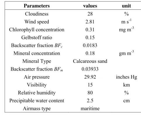
This research focuses on clarifying the role that the radiative transfer plays in calculating MLD in ocean circulation model. Therefore, the water constituents are assumed to be homogeneous in the water column. Table 3.1 lists the value of each parameter used in our model of underwater scalar irradiance. The model is able to consider a large variety of parameters that are currently not available from the observations, such as the chlorophyll and mineral concentration. A set of typical values of Case I water is used as a start. Detailed values of these parameters are expected to be generated from the biogeochemical model in the future. Some parameters should be updated at every time step, such as the wind speed and
11
cloudiness. As a starting point, we also set a set of typical values for those parameters for the entire simulation. Although the simulation can also be improved by resolving those parameters at every time step, the sensitivity test shows that the current values of parameters give comparable results to the observations. Note that the sun zenith angle is updated at every time step, because the earlier work indicates that sun zenith angle plays an important role in the distribution of underwater light field.
The model was original written in C++ language with a large look-up-table. This model has been rewritten to an independent function that can be called by the mixed layer model written in other language. To avoid errors in passing data across two models written in different language, we use the C++ version of the mixed layer model. At every time step, the model of underwater scalar irradiance is called first to calculate the profile of scalar irradiance, as well as the ideal value of surface irradiance. These values are then passing back to the mixed layer model and the entire profile is scaled according to the ratio of the ideal surface irradiance and the observed surface irradiance at that time step. All the rest of the mixed layer model is kept the same for comparison.
12
Parameters values unit
Cloudiness 28 % Wind speed 2.81 m s-1 Chlorophyll concentration 0.31 mg m-3 Gelbstoff ratio 0.15 Backscatter fraction BFc 0.0183 Mineral concentration 0.18 gm m-3 Mineral Type Calcareous sand
Backscatter fraction BFm 0.03933
Air pressure 29.92 inches Hg
Visibility 15 km
Relative humidity 80 %
Precipitable water content 2.5 cm Airmass type maritime
Table 3.1 A list of the parameters used in our model of underwater scalar irradiance.
13
Chapter 4. TOGA COARE observations
本 研 究 使 用 TOGA (Tropical Ocean - Global Atmosphere) 研 究 計 畫 的 IMET(Improved Meteorological Surface Mooring)浮標的觀測資料,浮標位於南緯 1°45´,東經 156°。TOGA 研究計畫在西太平洋暖池地區(western tropical Pacific warm pool),使用許多海洋以及大氣的觀測儀器,進行海洋-大氣偶合反應實驗 (Coupled Ocean–Atmosphere Response Experiment, COARE),主要目的為研究海洋 與大氣之間的交互作用情形,特別是聖嬰現象(El Nino)對此地區的氣候影響,所
設計的觀測實驗。整個實驗的觀測期間為 4.5 個月,從 1992 年 10 月 21 日
04:00UTC 到 1993 年 3 月 3 日 23:00UTC(此為國際標準時,非 local time),使用許 多 大 氣 、 海 洋 的 觀 測 儀 器 , 在 氣 象 學 方 面 的 觀 測 資 料 有 : 空 氣 溫 度(Air Temperature)、相對溼度(Relative Humidity)、氣壓(Barometric Pressure)、海溫(Sea Temperature,海水面以下 0.45m)、水平風速(Wind Speed)與風向(Wind Direction)、 入 射 的 太 陽 短 波 輻 射(Incoming Shortwave ; Solar) 、 長 波 輻 射 ( Longwave Radiation)、降雨率(Precipitation rate),每 7.5 分鐘觀測一次,詳細測量高度及儀
器名稱如表1 所示。同時,IMET 浮標在海面下也有掛載海洋觀測儀器,主要測
量:空氣溫度(air temperature)、氣壓(barometric pressure)、長波輻射(longwave radiation) 、 降 雨 (precipitation) 、 相 對 溼 度 (relative humidity) 、 太 陽 短 波 輻 射 (shortwave radiation, Solar), 海表面溫度(sea-surface temperature, SST)、風速及方 向(wind speed and direction),浮標從海下 0.4 公尺至 260 公尺,共掛有 46 個觀
測儀器,每15 分鐘觀測一次,詳細觀測資料如表 2。
但該浮標於1992 年 12 月 9 日 00:45UTC 到 12 月 13 日 05:25UTC 期間進行
維護,有缺少觀測數值的情形發生。因此,我們將採用鄰近的Tropical Atmosphere
14
Height (m) Variable Instrument
3.54 longwave radiation VAWR
3.54 shortwave radiation VAWR
3.54 wind speed VAWR
3.54 wind direction VAWR
3.0 barometric pressure VAWR
2.74 relative humidity VAWR
2.78 air temperature VAWR
3.14 precipitation IMET-1
-.45 sea temperature TPOD
Table 4.1 TOGA COARE 觀測資料表。儀器名稱:VAWR, Vector Averaging Wind Recorder Sensor;TPOD, Brancker Temperature recorder,主要測量溫度。
15
觀測資料(Parameter) 儀器(Sensor Type)
Air temperature Platinum Resistance Thermometer
Relative humidity Rotronic MP-100F
Barometric pressure Quartz crystal
Wind speed Wind monitor
Wind direction Wind monitor
Short-wave radiation Temperature compensated Thermopile Eppley
Long-wave radiation Pyrgeometer
Sea temperature Platinum Resistance Thermometer Precipitation Self-siphoning rain gauge
Aspirated air Platinum Resistance Thermometer with R. M. Table 4.2 IMET 觀測資料表。(http://kuvasz.whoi.edu/uopdata/coare/coare.html)
16
Chapter 5. Results and discussion
The radiative transfer model described in Chapter 3 is imbedded into the Mellor-Yamada level 2.5 one-dimensional mixed-layer model, as described in Chapter 2. The time series observations collected in the TOGA COARE from 1992 to 1993 are used to initialize and drive the model. The simulated profiles of density, salinity, temperature and velocity are then compared to the TOGA COARE observations to assess the model performance. In this report, we present and discuss the result of MLD since our focus is to clarify the role that the radiative transfer plays in calculating MLD in ocean circulation model. The results from another run of the mixed-layer model with default setting of K values as Jerlov’s type I water are also plotted for comparison.
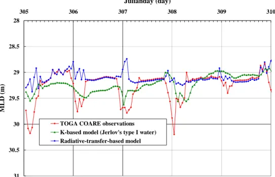
28 28.5 29 29.5 30 30.5 31 305 306 307 308 309 310 Julianday (day) ML D (m )
TOGA COARE observations K-based model (Jerlov's type I water) Radiative-transfer-based model
Figure 5.1 Comparison of the MLD between the TOGA COARE observations and the results simulated from the K-based model and the radiative-transfer-based model. Day 305 to Day 310.
To give a better resolution for each time step, Fig. 5.1 only shows the result from the first five days of simulation (day 305 to day 310). The K-based model gives a
17
similar trend to the observations. However, the simulated MLDs are deviated to the observations and generate an apparent phase lag. The MLD obtained from the radiative-transfer-based model, by contrast, is very close to the observations during the day time when the MLD is shallower than the the MLD in the night time. However, when the MLD starts to deepen, our simulation gives an opposite simulation. Since there is no way for the solar radiation to influence the MLD during the nighttime, there might be another mechanism in the one-dimensional mixed-layer model needs to be examined. One possible factor is the diffuse coefficient. Further works are needed to modify the one-dimensional mixed-layer model.
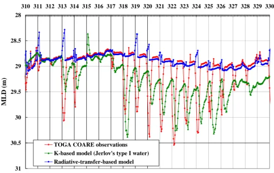
28 28.5 29 29.5 30 30.5 31 310 311 312 313 314 315 316 317 318 319 320 321 322 323 324 325 326 327 328 329 330 Julianday (day) ML D (m )
TOGA COARE observations K-based model (Jerlov's type I water) Radiative-transfer-based model
Figure 5.2 Comparison of the MLD between the TOGA COARE observations and the results simulated from the K-based model and the radiative-transfer-based model. Day 310 to Day 330.
Fig. 5.2 shows the result from day 310 to day 330. There is a special event during Day 314 and 315, of which the regular deepening of MLD during the nighttime is absent. As a result, the simulation result from the K-based model exhibits a substaintial deviation from the observations and getting worse and worse from then on. By contrast, the the radiative-transfer-based model gives a simulation that is much
18
closer to the observations. Especilly during the special event when there is no MLD deepening during the night time, such as the day 315 and day 329, the simulation from radiative-transfer-based model matches observations very well on both days. Note that a small deviation in the MLD shows from the Day 319. The systematic deviation might be the result of changing of water constituents, especially the biological part.
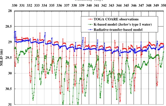
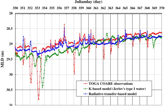
Another intereting phenomenon that has never been discussed before is the overshooting of MLD early in the morning. According to the observations, there will be such an event for every three days or so. The sampling interval of current observation might not be enough to resolve the event. However, this would be an ideal phenomenon to inveistigate by introducing a better model of underwater light field. Fig. 5.4 to Fig. 5.7 shows the comparison of the rest of the TOGA COARE observation. Basically, they all follow the same trend as discussed in Fig. 5.1 to Fig. 5.3. The systematic deviation between our model and observations, again, might be the result of changing of water constituents, especially the biological part.
28 28.5 29 29.5 30 30.5 31 330 331 332 333 334 335 336 337 338 339 340 341 342 343 344 345 346 347 348 349 350 Julianday (day) ML D (m )
TOGA COARE observations K-based model (Jerlov's type I water) Radiative-transfer-based model
Figure 5.3 Comparison of the MLD between the TOGA COARE observations and the results simulated from the K-based model and the radiative-transfer-based model. Day 330 to Day 350.
19 28 28.5 29 29.5 30 30.5 31 350 351 352 353 354 355 356 357 358 359 360 361 362 363 364 365 366 367 368 369 370 Julianday (day) ML D (m )
TOGA COARE observations K-based model (Jerlov's type I water) Radiative-transfer-based model
Figure 5.4 Comparison of the MLD between the TOGA COARE observations and the results simulated from the K-based model and the radiative-transfer-based model. Day 350 to Day 370. 28 28.5 29 29.5 30 30.5 31 370 371 372 373 374 375 376 377 378 379 380 381 382 383 384 385 386 387 388 389 390 Julianday (day) ML D (m )
Figure 5.5 Comparison of the MLD between the TOGA COARE observations and the results simulated from the K-based model and the radiative-transfer-based model. Day 370 to Day 390.
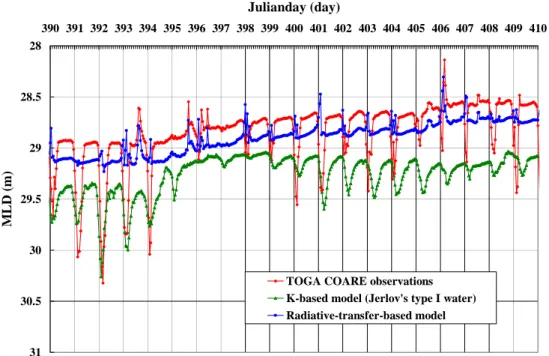
20 28 28.5 29 29.5 30 30.5 31 390 391 392 393 394 395 396 397 398 399 400 401 402 403 404 405 406 407 408 409 410 Julianday (day) ML D (m )
TOGA COARE observations K-based model (Jerlov's type I water) Radiative-transfer-based model
Figure 5.6 Comparison of the MLD between the TOGA COARE observations and the results simulated from the K-based model and the radiative-transfer-based model. Day 390 to Day 410. 28 28.5 29 29.5 30 30.5 31 410 411 412 413 414 415 416 417 418 419 420 421 422 423 424 425 426 427 Julianday (day) ML D (m )
TOGA COARE observations K-based model (Jerlov's type I water) Radiative-transfer-based model
Figure 5.7 Comparison of the MLD between the TOGA COARE observations and the results simulated from the K-based model and the radiative-transfer-based model. Day 410 to Day 427.
21
Chapter 6. References
1. Ackleson, S.G., 2001. Ocean optics research at the start of the 21st century. Oceanography, 14(3): 5-8.
2. Carder, K.L., Liu, C.-C., Lee, Z.P., English, D.C., Patten, J., Chen, R.F., Ivey, J.E. and Davis, C.O., 2003. Illumination and turbidity effects on observing faceted bottom elements with uniform Lambertian albedos. Limnology and
Oceanography, 48(1, part 2): 355-363.
3. Fasham, M.J.R., Ducklow, H.W. and McKelvie, S.M., 1990. A nitrogen-based model of plankton dynamics in the oceanic mixed layer. Journal of Marine Research, 48: 591-639.
4. Jerlov, N.G., 1976. Marine Optics. Elsevier, Amsterdam, 231 pp.
5. Lee, Z.P., Carder, K.L. and Arnone, R.A., 2002. Deriving inherent optical properties from water color: A multi-band quasi-analytical algorithm for optically deep waters. Applied Optics, 41(27): 5755-5772.
6. Liu, C.-C., 2006. Fast and accurate model of underwater scalar irradiance for stratified Case 2 waters. Optics Express, 14(5): 1703-1719.
7. Liu, C.-C., Carder, K.L., Miller, R.L. and Ivey, J.E., 2002. Fast and accurate model of underwater scalar irradiance. Applied Optics, 41(24): 4962-4974. 8. Liu, C.-C., Woods, J.D. and Mobley, C.D., 1999. Optical model for use in oceanic
ecosystem models. Applied Optics, 38(21): 4475-4485.
9. Mellor, G.L., 1991. An equation of state for numerical models of oceans and estuaries. Journal of Atmospheric and Oceanic Technology, 8: 609-611. 10. Mellor, G.L., 1998. Users guide for a three-dimensional, primitive equation,
numerical ocean model, Princeton University, NJ.
11. Mobley, C.D., Gentili, B., Gordon, H.R., Jin, Z., Kattawar, G.W., Morel, A., Reinersman, P., Stamnes, K. and Stavn, R.H., 1993. Comparison of numerical models for computing underwater light fields. Applied Optics, 32(36):
7484-7504.
12. Mobley, C.D. and Sundman, L.K., 2001. Hydrolight 4.2 Users' Guide, Sequois Scientific, Inc., Redmond WA.
13. Paulson, C.A. and Simpson, J.J., 1977. Irradiance measurements in the upper ocean. Journal of Physical Oceanography, 7: 952-956.
22
計 畫 成 果 自 評
本計畫之研究內容與原計畫相符,並順利達成預期目標。主要研究成果為將 一個運算速度快而且精確度高的輻射傳輸模式與一個一維海洋混合層模式相結 合,先透過參數靈敏度的測試以瞭解一維海洋混合層模式中各項計算條件受輻射 傳輸模式的影響。再其結果和實測溫度、鹽度與流速等資料加以比對,以評估使 用了輻射傳輸模式來計算水下光場的作法,是否提升了原來海洋混合層模式的準 確性。本研究可增進吾人對混合層深度受水下光場影響之瞭解,並可提升海洋環 流模式之準確性,極具學術與應用價值。現正整理研究內容,並尋求在國際學術 期刊發表。23
附 件 : 出 席 國 際 學 術 會 議 心 得 報 告
2005 AGU Fall Meeting 與會心得
成功大學地球科學系 劉正千 助理教授
美國地球物理學會(American Geophysical Union, AGU)秋季會議每年固定 12 月上旬於美國舊金山舉行。該會議幾乎包含所有地球科學相關課題,如地球、海 洋、大氣、太空和天文等,是每年地球物理界的一大盛事。
本校地科系劉正千助理教授,榮幸獲國科會補助參與 2005 AGU Fall Meeting。由 劉正千老師擔任第一作者之論文「輻射傳輸對海洋環流模式中混合層深度計算之 敏感度」(Sensitivity of radiative transfer on calculating MLD in ocean circulation model)通過大會審查,獲正式邀請,於會中以口頭報告之方式發表。藉由親自參 加會議,可與國際上相關研究人員交換研究心得,更可增加未來參與國際上大型 合作計畫之機會。本次會議中欣見國內中研院、台大、成大、中正及中央等學術 研究單位合計超過五十位代表與會。大家於會議中分享交流心得、獲益匪淺。亦 於會場中見到多位過去在國外工作時的研究夥伴,互道近況,並尋求未來合作的 可能機會。 參加國際學術會議是提昇研究水平,並且與國際接軌的重要途徑,參加此次會議 欣見許多來自國內的學生與會,相信必對他們未來的學術生涯裨益甚多。茲將本 次參加會議所發表之論文摘要附加於本心得報告之後。
1
depths in ocean circulation model
Cheng-Chien Liu and Wei-Chih Lin
Department of Earth Sciences, National Cheng Kung University, No. 1, Ta-Hsueh Road, Tainan, TAIWAN 701 R.O.C.
2
The ocean circulation model has been widely employed to simulate and forecast the oceanic environment, which enables the assessment of roles that various factors play in climate change, such as the budget of carbon dioxide and the resumption of thermohaline. Success of this approach relies on an accurate simulation of mixed layer dynamics that dominates the major physical and biogeochemical processes in the upper ocean. Sunlight is the main source of natural energy that heats the seawater and causes the vertical convection. Advances in radiative transfer modeling and theory in the past two decades have now enabled a realistic simulation of underwater light field by solving the full radiative transfer equation. This paper incorporates the radiative transfer model into the Mellor-Yamada level 2.5 one-dimensional mixed-layer model. The time series observations collected in the Tropical Ocean Global Atmosphere Coupled Ocean Atmosphere Response Experiment (TOGA COARE) from 1992 to 1993 are used to initialize and drive the model. The simulated profiles of density, salinity, temperature and velocity are then compared to the TOGA COARE observations to assess the model performance. Success of this research will clarify the role that the radiative transfer plays in calculating mixed-layer depths in ocean circulation model.