颱風及極端降雨在翡翠水庫中經由上行效應對浮游生物的影響

(1)

國立臺灣大學理學院海洋研究所碩士論文

Graduate Institute of Oceanography College of Science

National Taiwan University Master Thesis

颱風及極端降雨在翡翠水庫中經由上行效應對浮游生物的影響

Influences of typhoons and extreme rains on plankton through bottom-up effects in Feitsui Reservoir

黃煒忠

Wei-Chung Huang

指導教授：謝志豪博士 Advisor: Chih-hao Hsieh, Ph.D.

中華民國 104 年 7 月

July, 2015

(2)

I

致謝

這篇論文能夠完成，首先就要感謝的就是謝志豪老師，感謝老師能在碩士期間給我許多學術上的指導，以及在父親生病期間給我很大的包容。另外還有在統計跟實驗上我許多建議與幫助的俊偉學長、蔡政翰學長，在論文修改上給我很多幫助的雹舜、佩軒&榮恩、澗庚，陪我度過這段時間的實驗室夥伴拉狗、冠婷，

以及幼青、小平、口天、貓、奧斯卡、怡君、梵絃、蘇民弦等歡樂422 的大家，

中研院一起去翡翠採樣的夥伴們，還有生科 B96 的同學們，還有最重要的我的

家人，感謝各位陪伴我走過這四年，真的是謝謝大家了。

(3)

II

Abstract

The frequency of extreme weather events has increased due to climate change, resulting in strong disturbances in ecosystems. Extreme precipitations (EP) in lake systems caused by typhoons and extreme rains (ER) represent a pressing concern.

Previous studies indicate that EP can cause disturbances to phytoplankton communities owing to increased turbidity (OBS) and nutrients (PO43-) coming from upper streams. However, whether and how these bottom-up effects can be transferred to zooplankton remains elusive. To tackle this issue, we investigated the zooplankton communities, phytoplankton biomasses, and environmental factors in both the pre-EP and post-EP periods of multiple EP events from 2008 to 2012 in Feitsui Reservoir. We found that, in general, turbidity and PO43- increased after EPs. Meanwhile, chlorophyll a decreased immediately after EPs due to light blocking effects and then gradually recovered to its original level in two weeks. In addition, the depth of chlorophyll a maximum decreased about 6 meter after typhoons. These two responses of chlorophyll a indicated that phytoplankton were mainly affected by turbidity immediately after EPs. More importantly, we found that zooplankton showed differential responses to EP events depending on their body size and feeding habit.

More specifically, the species composition of zooplankton shifted to being dominated by smaller species after typhoons and extreme rains. This compositional shift resulted

(6)

V

in a decrease in the total biomass, although the total abundance was increased. In addition, species composition of zooplankton changes significantly between the pre-EP, post-EP, and normal periods, as shown by the discriminant analysis. These findings indicated that EP events altered the physical and chemical conditions of lake environment and the disturbance can be transferred to phytoplankton and zooplankton.

Both phytoplankton and zooplankton decreased in abundance, and in addition, zooplankton changed their size and species composition.

Keywords: typhoon, extreme precipitation, bottom-up effect, phytoplankton, zooplankton, deep lake, Feitsui reservoir, species composition.

(7)

VI

中文摘要

由於氣候變遷，極端氣候出現的頻率也隨之增加，這些極端氣候對生態系會造成強烈的擾動。例如在湖泊生態系中，由颱風(typhoon)以及大雨(extreme rain, ER)事件所造成的強降雨(extreme precipitation, EP)，其所造成的影響儼然已成為

重要議題。之前的研究指出，強降雨可以經由讓濁度上升以及由上游帶來營養鹽來對浮游植物群集造成擾動(disturbance)。然而，關於這種上行效應(bottom-up effect)是否傳遞到浮游動物以及如何傳遞的機制仍然不清楚。為了解決這個議題，

我們利用在2008 到 2012 年間在翡翠水庫發生的強降雨事件，調查了在這些事件

中的強降雨前期和強降雨後期裡浮游動物群集、浮游植物生物量以及環境因子變化間的相關性。我們發現，通常濁度(turbidity)跟磷營養鹽(phosphate)會在強降雨 之後上升，同時葉綠素 a 的濃度在強降雨過後由於光遮蔽效應而迅速下降，然後 再漸漸回復至強降雨事件前原本的濃度水平。另外葉綠素 a 的最大值深度(the depth of the chlorophyll a maximum)也在颱風後顯著變淺。葉綠素 a 濃度跟最大值 深度的變化說明了浮游植物主要是受到強降雨帶來的濁度上升所影響。更重要的是，浮游動物會根據其體型大小跟食性對強降雨產生不同的反應。強降雨後浮游動物的總密度上升但總生物量下降，說明了其物種組成會在強降雨後偏向較小尺寸的物種如輪蟲或小型枝腳類。我們也利用判別分析發現浮游動物的物種組成在強降雨事件後跟平日間有顯著的差異(正確率超過 80%)，將強降雨事件後再細分為四個時期(以週為單位)後，每個時期彼此間的重分類正確率也接近 70%。這些

(8)

VII

發現提供了強降雨會在湖泊中造成擾動且這些擾動會經由上行效應影響浮游動物的量及組成的證據。

關鍵字：強降雨、颱風、上行效應、浮游動物、浮游植物、深水湖泊、翡翠水庫、

物種組成。

(9)

1

Introduction

The effects of typhoons on ecosystems have become an increasingly important issue due to the fact that the frequency and intensity of strong typhoons have increased significantly in recent years (Webster et al. 2005, Elsner et al. 2008).

Typhoons play an important role in disturbing lake ecosystems, particularly in Taiwan (Tsai et al. 2008). The main effects of typhoons on lake ecosystems consist of two components: winds and precipitations. However for deep lakes, the effect of wind may not be critical, because winds cannot cause vertical mixing strong enough to induce changes in deep lakes (Hansen 1975). For example, Robarts et al (1998) found that the shallow basin showed a significant phosphate increase resulted from typhoon-triggered resuspension and verical mixing, whereas the deep basin did not.

Thus in this study, we do not consider the effects of winds because Feitsui Reservoir is deep (mean depth = 40 m, maximum depth = 100 m) and relatively small (water area = 10.24 km²).

Regarding precipitation effects, recent studies have shown that a large amount of upstream inflow induced by typhoons and extreme rains (ERs) can change particle dynamics through resuspension and chemical dynamics such as increased dissolved oxygen (DO), dissolved organic carbon (DOC), phosphorus, and nitrogen concentration (Robarts et al. 1998, Satoh et al. 2001, Fan and Kao 2008, Tseng et al.

(10)

2

2010, Fan 2011, Yang et al. 2011). For example, a study of Lake Onogawa in Japan showed that extreme rains resulted in vertical mixing because of a huge water inflow, and increased amounts of particulate components, such as suspended solids, particulate carbon, particulate phosphorus, and particulate nitrogen in the whole water column after the typhoon (Satoh et al. 2001). The rainfall-driven hydrological effects induced two key bottom-up effects in the lake ecosystems: (1) increased turbidity (Jewson and Taylor 1978, Liboriussen and Jeppesen 2003) and (2) nutrients load (Hecky and Kilham 1988, Rosemond et al. 1993).

As for the biotic aspect, the phytoplankton community is affected by typhoons, but the mechanism of typhoon effect and the response of phytoplankton could be different according to physical and chemical characteristics of different lakes and different phytoplankton groups (Frenette et al. 1996, Nakano et al. 1996, Sakamoto and Inoue 1996, Seike et al. 1996). For instance, studies of Lake Biwa, Japan (Frenette et al. 1996, Nakano et al. 1996, Sakamoto and Inoue 1996, Seike et al. 1996), and Lake Apopka, Florida (Carrick et al. 1993, Schelske et al. 1995) have suggested that abundance of phytoplankton increased after typhoons due to increased nutrients or recruitment of resting cells caused by sediment resuspension. In contrast, a study of Lake Okeechobee, Florida has shown that the phytoplankton abundance decreased after typhoons due to light blocking effects resulted from high turbidity caused by

(11)

3

sediment resuspension (Havens et al. 2011), and another study of an alpine lake in northern Taiwan has shown that the gross primary production (GPP) decreased after typhoons due to low photosynthesis efficiency resulted from light blocking effects and chlorophyll a decreased because phytoplankton was flushed out in a very shallow lake (4.5 m maximum depth) (Tsai et al. 2008, Tsai et al. 2011).

Although studies on typhoons abound, previous studies paid relatively little attention to typhoon effects on zooplankton. Studies in shallow lakes have shown that the zooplankton biomass increased (James et al. 2008, Havens et al. 2011) and the lake metabolism became more heterotrophic after typhoons (Tsai et al. 2011). The studies of deep lakes usually emphasize on physical environments (Fan and Kao 2008, Tseng et al. 2010, Fan 2011, Yang et al. 2011), and have limited discussion on the biotic components (Wu and Chou 1998). However, whether and how the bottom-up effects propagate from nutrients to zooplankton in lakes remains unclear. Few studies have attempted to investigate the effects of typhoons on zooplankton in lakes. The study addressing this issue was carried out in Lake Biwa and the results showed that the typhoon exerted no significant influence on the zooplankton community, although the horizontal distribution of zooplankton changed (Kawabata and Urabe 1996). As zooplankton play an important role in food webs (Carpenter et al. 1985, McQueen and Post 1988), further investigation into the effects of typhoons on the composition and

(12)

4

abundance of zooplankton is needed.

There are some advantages to use zooplankton community as an indicator to investigate the effect of disturbance. First of all, zooplankton community is relatively easy to monitor than other large mobile animals (Sousa 1984). Secondly, a shorter life span and faster succession rate of zooplankton yield a faster response rate, which makes the observation easier. Third, the zooplankton community not only structures phytoplankton community through top-down control (Briand and Mccauley 1978, Sterner 1989) but also mediates energy flow from the lower to higher trophic level (Gliwicz and Pijanowska 1989). Therefore, zooplankton community is a good bioindicator for observing ecosystem responses to disturbances.

By examining the dynamics of zooplankton in Feitsui Reservoir, we aim to investigate the mechanisms and effects of typhoons and extreme rains (ER) on the zooplankton community in a subtropical deep reservoir. To tackle this issue, we contrast the zooplankton community before extreme precipitations (EP, including typhoon and ER, Table 1) with that after EPs for multiple EP events from 2008 to 2012 in Feitsui Reservoir, northern Taiwan. In lake ecosystems, zooplankton communities are often dominated by cladocerans, copepods, and rotifers (Molinero et al. 2006, Anneville et al. 2007, Winder et al. 2009), which were the target species of this study.

(13)

5

We tested the following hypothesis: a large amount of upstream inflow caused by EPs results in high turbidity (Satoh et al. 2001, Fan 2011, Havens et al. 2011, Yang et al. 2011) and increased nutrients, yet only one of these two effects would be transferred to biological components such as phytoplankton and zooplankton community. There are two possible situations of ecosystem in Feitsui Reservoir after EPs: (1) the turbidity dominant situation or (2) nutrient dominant situation. In a deep subtropical lake, turbidity may cause the total chlorophyll a to decrease and the chlorophyll a maximum depth to become shallower because of the reduced light availability. Under this light limited condition, the abundance of phytoplankton (Vinyard and O’brien 1976, Miner and Stein 1993, Dokulil and Padisak 1994, Havens et al. 2011) and zooplankton (Hart 1986, Kirk 1992, Jack and Gilbert 1993) decrease.

Yet, the zooplankton might respond differentially according to not only their body size because smaller species usually has higher metabolic rate and short life span (Gillooly et al. 2001, Speakman 2005) but also their feeding behavior because zooplankton growth and productivity are suppressed by suppressing food availability resulted from shading of light, especially on filter-feeing zooplankton (Wetzel 2001).

For instance, abundant silt particles overwhelm phytoplankton particles during flooding events decreased longevity, recruitment, and fecundity of some cladocera species (Threlkeld 1986, Kirk 1992). Phytoplankton decrease because their

(14)

6

photosynthesis cannot perform efficiently in the light limited environment.

Herbivorous zooplankton also decrease after food resources have been reduced, followed by a decrease in the abundance of carnivorous zooplankton. In contrast, increased nutrient concentrations may bring about phytoplankton blooms (Dokulil and Padisak 1994, Tanaka et al. 1996, Satoh et al. 2001) or change phytoplankton composition (Frenette et al. 1996), and the bottom-up effect of nutrient enrichment can be transferred to higher trophic levels such as zooplankton (Burgi et al. 1999). As a consequence, both phytoplankton and zooplankton may increase.

(15)

7

Materials & Methods

Study Site

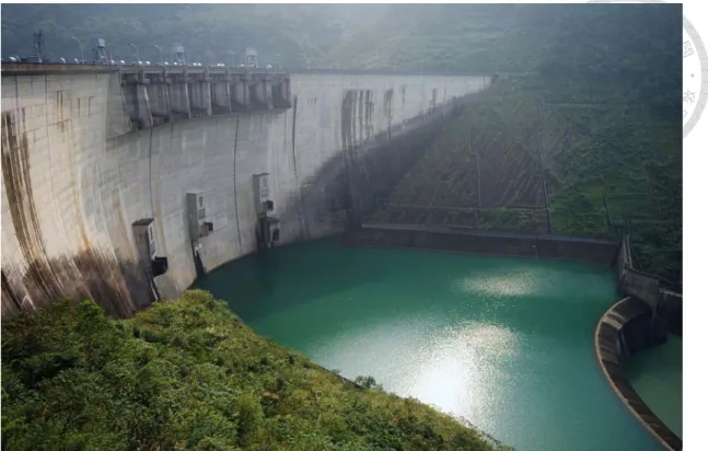
Feitsui Reservoir is a stratified dam-construct reservoir located in northern Taiwan (121° 34’ E, 24° 54’ N) at an altitude of 170 m above sea level (Fig. 1), and has a catchment area of 303 square kilometers (Chang et al. 2014) and is on average 90 meter deep (maximum depth 100 m). According to the data in 2005, the proportion of land use of the catchment area is forest (85.9%), farmland (6.6%), water mass (3.7%), grassland (2.6%), and market (1.1%) (Chen et al. 2013). The dam is located in the downstream valley of three major tributaries of the Xindian River, the Kingkwa Creek, the Diyu Creek, and the Peishih Creek. This reservoir was constructed in 1987 and then became the major drinking water source for more than 5 million people in the Taipei metropolis (Fig. 2); therefore, water quality is so carefully protected and monitored that its trophic status is oligo- to mesotrophic according to the Carlson trophic state index (Carlson 1977, Wu and Chou 1998). The ratio of catchment area to surface area is about 30:1, which is more similar to natural lakes (10:1) rather than ordinary reservoirs (100:1 to 300:1) (Wetzel 2001). This low ratio between catchment area and surface area and the conservation of soil and water in catchment area might cause a longer residence time (268 days = 0.73 year) of Feitsui Reservoir (estimation based on data from 2008 to 2013), which is also similar to natural lakes (from one to a

(16)

8

few years) rather than ordinary reservoirs (typically from days to several weeks) (Wetzel 2001). Feitsui Reservoir experiences a high precipitation rate of about 3,700 mm per year. In addition, the major source of the precipitation is from typhoon rains in summer and autumn, and from cold front rains of northeastern monsoons in winter (Chen et al. 2006, Fan and Kao 2008). For example, two typhoons contributed to 1666 mm precipitation in September 2001, equaling to 32 % of the total rainfall in 2001 (Chen et al. 2006).

Sample Collection

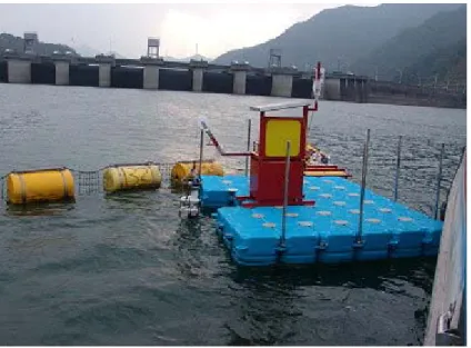
Our fieldwork sampling location, called dam site, was a moored monitoring platform located near the deepest point of the reservoir (Fig. 1, 3a), which is 1 km away from the dam of reservoir. In order to investigate the EP effects on the zooplankton community, we carried out sampling weekly in summer and biweekly in other seasons from January 2008 to August 2012. The physical and chemical data, including water temperature, photosynthetically active radiation (PAR), dissolved oxygen (DO), pH, and turbidity, were recorded by sensors of an in situ real-time monitoring CTD (conductivity, temperature, and depth) system (Fig. 3b). Both Total Suspended Matter (TSM) and OBS (Optical Backscatter Sensor) were measured to indicate the turbidity (Tanaka et al. 1996, Fan 2011); OBS is used as the turbidity

(17)

9

indicator in this study. Water samples collected by a 5-liter Go-Flo bottle from the 90, 70, 50, 30, 20, 15, 10, 5, 2, and 0 meter depth were used to measure nutrients, including dissolved inorganic nitrogen (DIN, including NO2 and NO3), phosphate (PO43-) and silicate (SiO3). DIN, silicate, and chlorophyll concentrations, following standard procedures (Parsons et al. 1984a, b, c, d, e, Gong et al. 1995, Tseng et al.

2010).

The zooplankton samples were collected by a 50-um mesh plankton net towed vertically from the 50 m depth to the surface, and the total volume of water passing through the net was recorded by a flowmeter equipped with the net. The density of

zooplankton was calculated by following equation (1), which gives us DenZ:

Den = N × (F − F ) × α × r × π × 1000 ×

----(1)

, where the NZ is the individual number of subsampled zooplankton, the Ffinal and Finitial are the reading of flowmeter, α is the coefficient of flowmeter, r is the radius of plankton net, Iv is the water volume used in zooplankton identification, and Sv is the water volume of condensed sample. Then we multiplied this equation by 1000 to convert the unit to individual L. The proportion of the amount of water to the volume of space towed by the net (net opening area* towing depth) is defined as filtration efficiency, and the average efficiency is 53% (Chang 2009, Chang et al.

2014). After the plankton sample was brought back to our laboratory, it was

(18)

10

concentrated to about 125 ml. Then, the sample was stored in a refrigerator at 4℃ for an hour followed by an addition of CO2 effervescing agent for anesthetization to prevent rotifers deformation. Lastly, the sample was fixed in 2% formalin. In each sampling date, we subsampled more than 300 individuals of zooplankton for species identification. The species identification was done under stereomicroscope following the published taxonomic key (Wang 1961, Chiang and Du 1979, Shen and Song 1979, Koste and Shiel 1987, Dussart and Defaye 2001), and adult individuals were identified to species level if possible. A microscopic CCD camera (Olympus DP71) was used to take images of zooplankton. These images were analyzed with the imaging analysis software (Olympus analySIS^®) to measure total length and width of each individual. We then used the empirical length-mass equations to estimate the carbon weight representing the biomass of crustacean zooplankter and rotifer (Dumont et al. 1975, Bottrell et al. 1976, Downing and Rigler 1984, Andersen and Hessen 1991).

Extreme Precipitation Index

From 2008 to 2012, almost all of the extreme precipitation (EP) events hitting Feitsui Reservoir brought heavy rainfalls to the catchment of the reservoir. The water surface area of Feitsai Reservoir is relatively small, and thus we consider that Feitsui

(19)

11

Reservoir was not significantly influenced by the winds of typhoon events. Therefore, we assumed the heavy rainfall to be the main influence from typhoons during our study period (Fig. 4a). While we mainly consider precipitation influence, we cognize that the rain intensity differs between typhoon and heavy rains. The discharge of water from upstream tributaries into Feitsui Reservoir exerted a direct influence of lake physics and chemistry in this deep lake system, and the discharge was highly correlated with the precipitation given that the time lag between the precipitation and the increased river discharge is only one day (correlation coefficient between precipitation and discharge of one day time lag = 0.692, two day = 0.573, three day = 0.281) (Fig. 5). Therefore, the precipitation could be used as an indicator of the magnitude of EP disturbance. We obtained the data for the precipitation in the watershed of Feitsui Reservoir from the Taipei Feitsui Reservoir Administration. The date with the highest averaged daily accumulated rainfall (ADAP) is defined as the typhoon hitting date. The data for typhoons were obtained from the Central Weather Bureau of Taiwan (CWBT) (http://rdc11.cwb.gov.tw/TDB/), and strength of a typhoon also follow its classification. The following criteria were used to define the strength of an extreme rain (ER) event: (1) Heavy rain: ADAP > 50 mm/day, (2) Extremely heavy rain: ADAP > 130 mm/day, (3) Torrential rain: ADAP > 200 mm/day, and (4) Extremely torrential rain: ADAP > 350 mm/day (http://www.cwb.gov.tw/V7e/

(20)

12

observe/rainfall/define.htm) (Tsai et al. 2011), as detailed in Table 1.

Data Analysis

Changes in biotic and abiotic variables resulted from EP events

To evaluate the influence of each EP event on Feitsui Reservoir, we chose 7 environmental variables, such as the level of TSM, OBS, DOC, PAR, nitrite, nitrate, and phosphate, as well as 4 biotic variables, including the biomass of bacteria, concentration of chlorophyll a, and density and biomass of zooplankton. We evaluated the difference in these variables between pre- and post-EP samplings, and evaluated the significance of difference by comparing them with the fluctuation in normal days (sampling dates not affected by typhoons or extreme rains), using a randomization test.

Because the influence of extreme rains is similar to that of typhoons, we pooled the data from typhoons and extreme rains together for statistical analysis, except for some specific analyses. First of all, the samples were classified into 2 groups: EP and normal period (if no EP event happened before a sampling within one month, this sampling would be defined as one of normal period). Secondly, for each EP event, we calculated the difference in each variable between pre-EP and post-EP samples in percentage with equation (1), which gives us CPEP:

CP ( ) =

^{( )}

× 100%

---(1)

(21)

13

, where Spre-EP is the closest pre-EP sample before an EP event (within two weeks), and Spost-EP(i) is the ith week post-EP sample of an EP event. Similarly, for the normal periods, we calculate the difference in each variable between any pair of two adjacent

samplings in percentage, which gives us CPnormal

CP ( ) = × 100%

---(2)

, where Si and Si-1 are the ith and i-1th samples collected during the normal period. We can then evaluate the significance of changes (mean CPEP – mean CPnormal) with randomization tests for each factor (Anderson 2001). In randomization test, the null model was constructed by pooling all CPEP and CPnormal, and then divided the pool randomly into CPEP* and CPnormal*. This step was repeated 1000 times to establish a null distribution of mean CPEP* － mean CPnormal*. We then compared our observation value with the null distribution and calculated the p-value.

The influence of EP events on abiotic factors and the phytoplankton community

To investigate the effects of EP, we further examined change percentages (CP) within 4 weeks after EP and compared these changes with normal days. We counted the number of increased and decreased CPs within the 4-week periods after EPs and calculated the ratio: _#^# (# = number). Similarly, we made the same

(22)

14

calculation for two consecutive sampling days during the normal period as a comparison. We then used the binominal test to detect whether the ratio for EPs is significantly different from that of the normal days. This analysis was done only for the variables that had passed the aforementioned randomization test. In binominal tests, we further divided EP into two categories: (1) typhoons and extreme rains, and (2) post-EP period into the disturbed (first week after an EP event) and recovering stages (second to fourth weeks after an EP event). In addition, we also examined the depths of chlorophyll a maximum in different stages after an EP event and in normal days. Using Dennett's test for the depth of chlorophyll a maximum, the normal days were used as the control group. In the Dennett's test, the depth of chlorophyll a maximum data within 4 weeks after ERs were aggregated into a single group, whereas the post-typhoon data were analyzed for the four weeks separately after a typhoon.

The influence of EP events on zooplankton abundance and biomass

To examine whether the bottom-up effect of EPs had influenced the zooplankton community or not, we used time series data of total density and biomass. We conducted linear regression and scatter plot between total density and total biomass of zooplankton after EPs. The relationship between total density and biomass in four different seasons was defined as the baseline for the comparison of EP effects versus

(23)

15

seasonal effects. The spring, summer, autumn, and winter were defined as: from March to May, from June to August, from September to November, and from December to February, respectively. Furthermore, we expressed the size data at log2

scale in both the pre-EP and 4 post-EP weeks. We classified the zooplankton population according to individual body weight (in pico-grams), and then grouped the size classes into five broad categories in order to compare the respective proportions of the total biomass and total number of individuals. The “largest” category (defined as that of individuals of weight > 2²¹ pico-grams) includes herbivorous calanoid adults and large cladocerans, the “large” category (defined as that of individuals of weight between 2¹⁷ to 2²¹ pico-grams) includes small herbivorous cladocerans, copepodites and large nauplii, and carnivorous cyclopoid adults, the “middle”

category ( 2¹³< weight < 2¹⁷ ) includes small nauplii and most rotifers, the “small”

category ( 2⁹ < weight < 2¹³ ) includes small rotifers. The “smallest” category includes individuals of body weight < 2⁹.

The influence of EP events on zooplankton composition

The discriminant analysis was used to analyze whether species composition had shifted after EP events and whether the changes were predictable. Firstly, we classified the samples into 6 groups according to the sampling time: pre-EP, first

(24)

16

post-EP week, second post-EP week, third post-EP week, fourth post-EP week, and normal periods. Secondly, after discriminant functions were derived, we visually inspected the group differences in a two-dimensional plot using their coefficients of the linear discriminants. We calculated correct classification rates to test the predictive performance of our discriminant functions. Prior to analysis, the variance of species abundance was homogenized and the rare species were down-weighted by the Hellinger transformation (Legendre and Gallagher 2001). Furthermore, to account for the unequal sample size in different groups, Cohen's kappa statistic was used to interpret the chance-corrected classification results (Titus et al. 1984).

After the analysis, the species ranking in the top 13 according to either species score from density data or species score from biomass mass were recognized as distinct species since their accumulated percentage of species score accounts for more than 80

% of total species score. The species score was calculated by the following equation:

SS = (SS in LD1) + (SS in LD2)

...(3) , where SS is species score, LD1 and LD2 represent the coefficients of linear discriminants in axis 1 and 2, respectively. Finally, we assessed if the change in composition of zooplankton was caused by seasonal effect; thus, the dispersion of each group in the first two dimensions was calculated by the following equation:

(25)

17

Dis = 2 × ∑ ∑

⁽ ⁾ ⁽ ⁾

( ) ...(4) where n is the total number of a group; xk and yk represent the kth sample position in LD1 and LD2 respectively (k=1,…, n-1). Equation 4 calculated the average of all pairwise distances of all samples in a group to represent the dispersion in the two-dimension plot. We then used the Tukey's ‘Honest Significant Difference’ (HSD) test to compare the variances among the groups.

(26)

18

Results

Effects of extreme precipitation (EP) events on environmental factors and phytoplankton

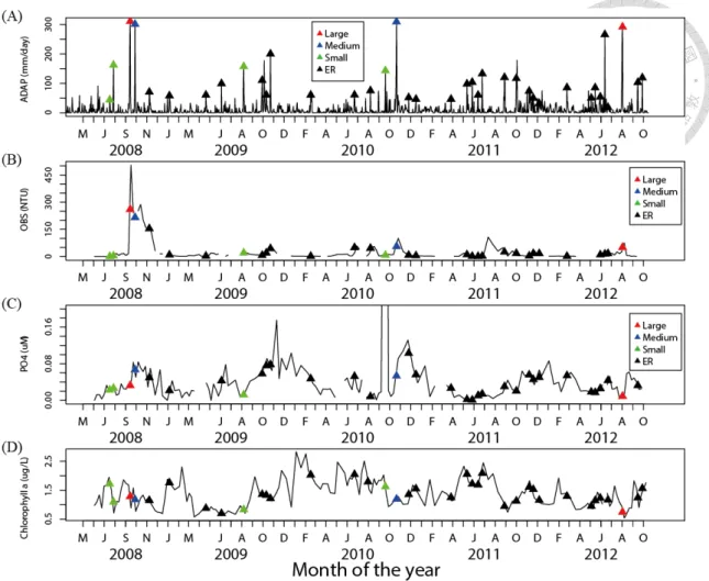
From 2008 to 2012, there are 38 EP events in Feitsui Reservoir, including 2 large typhoons, 2 medium typhoons, 4 small typhoons, and 30 ERs (Fig. 4a). After extreme precipitation (EP) events (closed triangles in Fig. 4a), turbidity, optical backscatter sensor (OBS), and phosphate increased substantially and then decreased gradually (Fig. 4b, c). In contrast, the concentration of chlorophyll a decreased sharply after typhoons and then recovered gradually (Fig. 4d). No effect from EPs was observed in the other observed environmental factors (specifically, DOC, PAR, NO2, NO3, bacterial production, and primary production).

Results of randomization tests indicate that the OBS and phosphate concentration (PO43-) exhibit significantly larger mean change percentage (CP) in the post-EP than in the normal periods (Table. 2, p<0.05). Other factors including dissolved organic carbon (DOC), photosynthetically active radiation (PAR), nitrite (NO2-) and nitrate (NO3-) concentrations, do not show any significant difference (Table. 2, p>0.05). In terms of biotic factors, bacteria biomass, phytoplankton (chlorophyll a) and zooplankton density and biomass show significantly higher CPs in the post-EP than in the normal periods (Table. 2, p<0.05).

(27)

19

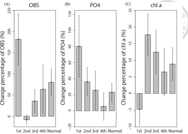
The CPs also yield information about the recovery process in the first four weeks after EPs (Fig. 6). OBS increased sharply to nearly 2 times higher than the original level in the first post-EP week and dropped rapidly to its pre-EP level in the second week (Fig. 6a). The phosphate level also increased in the first post-EP week, but then decreased gradually and did not recover to its pre-EP level until the fourth week (Fig. 6b). Chlorophyll a concentration dropped to 95% of its pre-EP level in the first week after EPs (dropped to 86% after typhoons), but increased to 120 % of its pre-EP level in the second week and decreased slowly until the fourth week (Fig. 6c).

The binominal tests corroborate the results (Table. 3). In the first post-EP week, both typhoons and extreme rains (ER) brought significantly more counts of increasing CP of OBS than normal days, but only typhoons caused significantly more counts of increasing phosphate (Table. 3a, b). In contrast, only ERs but not typhoons caused significantly more counts of increasing chlorophyll a concentration in the first post-EP week compared to normal days (Table. 3c). In the recovery stage (from the 2nd to the 4th weeks of post-EP period), only phosphate and chlorophyll a showed significantly or marginally significantly more counts of increase than normal days (Table. 3b, c). Moreover, when data from all weeks of post-EP were combined into one single category, only OBS and PO43- showed significantly and marginally significantly more counts of increase, respectively (Table. 3a, b).

(28)

20

The vertical profile of the phosphate and chlorophyll a

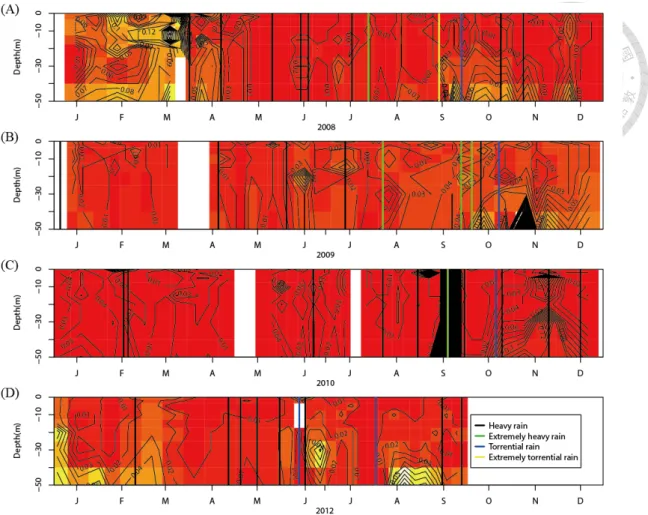
According to the vertical profile of phosphate concentration, we observed that phosphate concentration increased after EP events, especially after typhoons or large ERs, but mainly between the 30 to 50 meter depth (Fig. 8). Phosphate concentration was still low from the 0 to 30 meter depth after EP events, and only few EPs caused strong increase of phosphate in whole water column (Fig 8b, 8d). The vertical profile of phosphate also indicated that phosphate did not increase immediately after EPs but increased gradually after several days in the post-EP period.

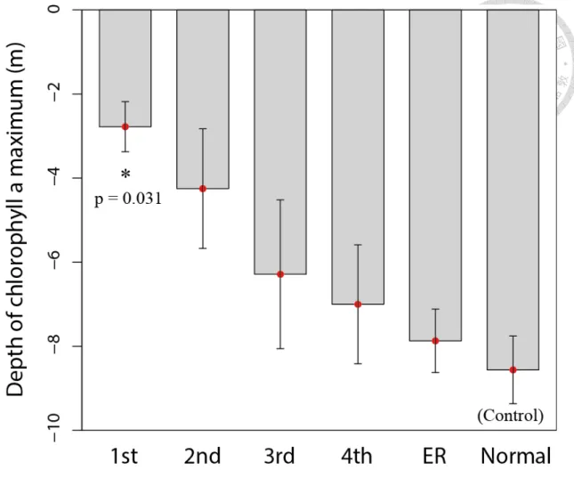
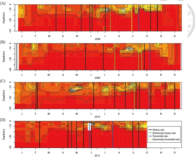
The depth of the chlorophyll a maximum decreased significantly in the first post-typhoon week compared to normal days (Fig. 7) (p = 0.031, Dennett's test), and increased gradually with time. Even though the chlorophyll a maximum descended to a depth of 7 meters in the fourth post-typhoon week, it was still less deep than in the normal days. Moreover, the vertical profile of chlorophyll a indicated that most phytoplankton usually lived in the depth between the 0 and 20 meter, and the chlorophyll a maximum usually appeared in the 10 ~ 15 meter depth (Fig. 9). In the post-EP period, the distribution of chlorophyll a became more close to the water surface, especially after strong typhoons and ERs (Fig. 9).

(29)

21

The response of zooplankton density and biomass to EP events

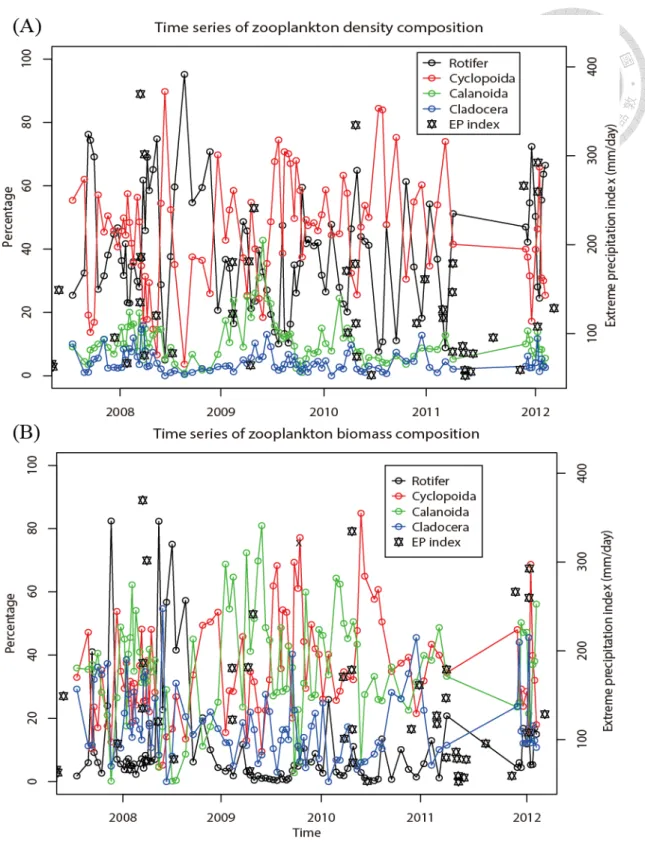
In the typhoon and extreme rain periods, the total density of zooplankton showed an increasing trend, but the total biomass showed a decreasing trend (Fig. 10).

However, when the total density and biomass were divided into 4 taxonomic groups (Rotifer, Cladocera, Cyclopoida, and Calanoida), no change in composition along the time series was revealed (Fig. 11a, b). When analyzing the CP of the total density and biomass in seasonal groups and in EP groups (typhoon, ER, and normal days), the result showed a positive correlation between the total density and the biomass in both the post-ER and normal days groups (Fig. 12a, b); in contrast, the post-typhoon group showed a significant negative correlation (Fig. 12b; p = 0.0156).

According to the x-y scatter plot and linear regression, the CPs of the total density and biomass of zooplankton showed opposite responses in the first post-EP week compared to those of any other two consecutive post-EP samples (Fig. 12). The change of the total density and the biomass showed a similar trend from the second week to the fourth week of the post-EP stage, and the proportion of individuals represented by the small-size category became higher in the fourth week (Fig. 13). At the first post-EP week, the decrease in the “largest” ( >2²¹) size category and the increase in the “large” size category ( 2¹⁷~2²¹) can account for the opposite trend in total density and biomass, despite the increase in the “middle” ( 2¹³~2¹⁷) category.

(30)

22

From the second week to the third week, both the “largest” ( >2²¹) and “middle” size categories ( 2¹³~2¹⁷) showed increasing trends, but the “large” category showed an opposite trend. Lastly, the “large” and “middle” size categories increased from the third week to the fourth week, but the “largest” category decreased.

The response of zooplankton species composition to EP events

Results of the discriminant analysis revealed the distinct species of zooplankton between the pre- and post-EP period. Six Rotifers species and one Cladocera species (Moina micrura) ranked in the top 13 according to both the density and the biomass data (Table 4). Our discriminant analysis was able to successfully distinguish between EP and normal periods, as well as between different stages of an EP event. When only EP and non-EP periods were taken into account, the correct classification rates for the density and biomass data were both over 80% (density data: 82.6%; biomass data:

84.8%). The chance-corrected classification rates based on Cohen's kappa were still 64.8% (for density data) and 69.6% (for biomass data) which are better than the results by chance (p < 0.001). Moreover, when the post-EP period was divided into 4 stages, the correct classification rates for distinguishing between any two of these 4 groups or between one of those groups and the normal days group according to density data and biomass data were both near 70% (density data: 69.6%; biomass data:

(31)

23

66.3%). Also, the rates calculated based on Cohen's kappa were 60.0% and 55.5%

according to density and biomass data respectively (Table. 5), which were significantly better (p < 0.001) than the results by chance.

As can be seen in Figure 14, the five groups of the change of species composition (including the four post-EP stages and normal days) can be discriminated visually from each other. Regardless of which dataset is considered, the two-dimension plot of discriminant analysis showed that the dispersion within group increased in post-EP period and the dispersion of the fourth week was significantly larger than that of normal days (Fig. 15). Overall, the normal-day group was discriminated from all post-EP stages in the discriminant analysis. Even though the normal-day group included days from all seasons of the year, the variance of normal days was not larger than that of the post-EP groups.

(32)

24

Discussion

The response of the environment and phytoplankton to EPs

We found that the turbidity and PO43- level increased and chlorophyll a concentration decreased immediately after extreme precipitation (EP) in Feitsui Reservoir due to light blocking effects and then gradually recovered to the pre-EP level. The result of the change percentage (CP) analysis clearly indicates that chlorophyll a concentration was strongly correlated with OBS (negatively) and PO43-

(positively) on a weekly time scale. The finding is consistent with previous studies in lakes (Scheffer 1998), rivers (Dokulil 1994), and estuaries (Cloern 1987).

Immediately after EPs in Feitsui, there was no relationship between the phosphate level and the chlorophyll a level, which is consistent with a previous study suggesting that phosphate did not critically influence phytoplankton in a high turbidity environment (Healey and Hendzel 1980), and the effect of phosphate needed longer time to appear. Moreover, the reason why we did not consider phosphate to be an important factor of chlorophyll a increase is that the distribution of phosphate (below 30 meter) is different from that of chlorophyll a (0 to 20 meter) according to the vertical profile of Feitsui Reservoir (Fig. 8, 9). Moreover, if the phosphate resulted from the influence of water discharge of turbidity current in mid-layer of water (Fan and Kao 2008) is critical for phytoplankton, one may expect that the distribution of

(33)

25

phytoplankton became deeper; however, this was not observed in our data. Thus, these findings indicate that the presence of strong light blocking effects caused by the high turbidity immediately after EPs is likely the key factor influencing the phytoplankton biomass.

We wish to emphasize that the physical mechanism of increased turbidity due to EPs in Feitsui Reservoir is quite different from that of shallow lakes. In shallow lakes, vertical mixing caused by high wind velocity could re-suspend sediments or increase turbidity directly and then create a light-limited environment even for several months (Havens et al. 2001, Havens et al. 2011, Tsai et al. 2011). In contrast, the Feitsui Reservoir is too deep to be affected by wind-induced vertical mixing; in fact, the enhanced turbidity came from upstream river discharge (Fan and Kao 2008). In the Feitsui Reservoir, even though the major turbidity current flowed into the mid-layer water because of its high density (Fan and Kao 2008), turbidity in the surface water was still elevated due to the run-off (Fig 4b, 6a).

Besides turbidity, the response of phosphate in the Feitsui Reservoir is also different from that in relatively shallower lakes. In the Feitsui Reservoir, after typhoons or extreme rains, phosphates flowed into the mid-layer of the reservoir following the aforementioned turbidity current. Then, the phosphates were transported upward and downward by diffusion and diurnal mixing (Chen and Wu 2003, Tseng et

(34)

26

al. 2010). The increase of phosphate concentration after typhoon at depths between 0 and 30 meters might be due to the upward transportation (Fig 4c, 6b). This explains why we found a positive correlation between phosphate levels and chlorophyll a levels a few weeks after EPs (after recovery from EP).

The light-limited environment due to high turbidity after typhoons had negative effects on the phytoplankton community in Feitsui Reservoir, by decreasing the total chlorophyll a (Fig. 4d, 6c) and the depth of the chlorophyll a maximum (Fig. 7). This situation then recovered gradually with positive CPs of phosphate concentration from the second to the fourth post-EP week. One may conjecture that the decreased depth of the chlorophyll a maximum may be related to the nutrient dynamics, as found in the Southern California Shelf where the vertical movement of the chlorophyll a maximum follows the thermocline and nutrient (Cullen et al. 1983). However, the decreased depth of chlorophyll a maximum in Feitsui Reservoir might not be due to the increase of phosphate in the post-EP period, because the depth of the phosphate inflow did not match the depth of chlorophyll a maximum (Fig. 8, 9).

In the binominal test, OBS, PO43-, and chlorophyll a showed different characteristics. For example, in normal days, OBS showed a downward change more frequently (ratio of _#^# = 0.563) because after a rain event the period of decreasing turbidity is longer than the period of increasing turbidity, and normal days

(35)

27

periods are composed of mostly sunny days and small rain events, as shown in other lakes (Robarts et al. 1998, Fan 2011). In contrast, OBS often showed upward change after EP (post-ER has a ratio of 1.385 and post-typhoon has a ratio of 2.5). The phosphate also showed more downward changes during normal days but this was not as obvious (ratio = 0.818) as in the case of OBS because phosphate had a longer increasing period, which represents a higher proportion of the post-EP event period (Robarts et al. 1998, Havens et al. 2011). In addition, upward changes in phosphate concentration occurred significantly more frequently after typhoons than after ERs, which might be the result of stronger rainfall intensity caused by typhoons compared to ERs. Generally speaking, with smaller precipitations, rainfall slowly infiltrates the soil matrix through capillary action, and the phosphate concentration of the flowing water decreases while water passes through soil matrix. As precipitation intensity increases, more water flows through macro-pores in shallower soil depths and carries more phosphate into the lake. (Gächter et al. 1998). Generally, typhoons have higher rainfall intensity compared to ERs, and the difference in intensity between typhoons and ERs results in distinct phosphate responses. In addition, the impact of these phosphate responses on phytoplankton is more significant during the second to the fourth week compared to the first week.

Chlorophyll a concentration usually showed more decreasing counts than

(36)

28

increasing ones in normal days albeit not so significant (the ratio for increasing/decreasing counts is 0.872), but its proportion of decreasing counts became even higher immediately after EP (post-ER has a ratio of 0.435 and post-typhoon has a ratio of 0.556). This phenomenon can be explained by the reduction of phytoplankton photosynthesis in light-limited environment, which limits the growth of phytoplankton, as described in previous studies (Cloern 1987, Dokulil 1994, Scheffer 1998). The ratio of increasing/decreasing counts in post-ER weeks was only marginally significant (p = 0.081), and the non-significant result in the case of post-typhoon weeks might be explained by the small sample size of typhoons (N = 14, from 2005 to 2012). In addition, counts of increasing chlorophyll a concentration were significantly more frequent in the post-typhoon recovering stage (ratio = 2.1; p = 0.018) than in the normal period. This can be explained by the gradual recovery of phytoplankton after the drop-off at the first post-typhoon week. In contrast, chlorophyll a concentration did not show significantly more increasing counts in the post-ER stage, the reason for which might be that phytoplankton decreased less, thus requiring less time for recovery. Briefly, the key driver influencing phytoplankton growth after EPs in the Feitsui Reservoir is turbidity.

The responses of zooplankton density and biomass to EP events

(37)

29

During the first week after an EP event, the total density and biomass of zooplankton showed contrasting trends. The zooplankton community passed through a fluctuation period to arrive at a composition with a higher proportion of individuals in the small size category, such as rotifers and copepod nauplii (Fig. 13a). In contrast, the time series data of four main taxonomic groups did not reveal any clear trend (Fig.

11); this might result from differing diets even within a taxonomic group. For instance, the diet of cyclopoida in different life stages changes from phytoplankton to zooplankton (Moriarty et al. 1973, Gophen 1977), different rotifer species have different feeding preferences (Starkweather 1980, Gatesoupe 1991, Duggan 2001), and different cladocera species prefer food particles of different sizes (Loedolff 1965, Gulati 1978, Bloem and Vijverberg 1984).

The total density and biomass showed opposite trends only in the first post-EP week, whereas in the recovery stage (from the 2nd week to the 4th week), they showed similar trends (Fig. 12). The decrease in the proportion of the largest and the middle size categories in the first week might have resulted from the shortage of food resource (phytoplankton) and the low feeding rate due to reduced light (Wetzel 2001), and the strength of their trophic link was stronger in meso-oligotrophic lakes such as Feitsui Reservoir than eutrophic lakes (McQueen et al. 1989, Carney and Elser 1990, Chen and Wu 2003). In addition, negative influence of turbidity on zooplankton

(38)

30

productivity and development is stronger than positive effect of nutrient enrichment on phytoplankton development (Wetzel 2001). For example, cladocerans growth and reproduction are severely restricted by the reduction of the feeding rate by 70%

induced by mechanical interference of suspended clay particles (Kirk 1992). The trend in the abundance of the large size category was not clear since that category includes both carnivores and herbivores. In the second week, the increase in zooplankton density and biomass mainly came from herbivores, whose resurgence was the result of their replenished food resource (McQueen et al. 1989, Carney and Elser 1990). Then, the total density and biomass collapsed in the third week because the population of herbivorous zooplankton increased, exceeding the carrying capacity of their food resource; similar phenomena induced by seasonal regulation and the predator-prey system have been observed and explained by biological modeling (Lampert et al. 1986, Luecke et al. 1990, Scheffer et al. 1997). After the collapse of the total density and biomass in the third week, the increase in the two smaller size categories (small and large) was the main reason for the recovery of both the total density and biomass in the fourth week. Previous studies have indicated that growth rates of small-size copepodites and nauplii were significantly higher, and the growth of the latter was even unlimited by food resources (Hopcroft and Roff 1998, Hopcroft et al. 1998). Moreover, growth rates of smaller rotifers were higher because they can

(39)

31

adapt to living in food-scarce environments. Larger rotifers cannot tolerate food shortage in early post-EP stages, so they die and cannot show high reproductive potential in further food-rich situation (Stemberger and Gilbert 1985). The recovery we observed in zooplankton mainly came from the smaller size category because of their short life span and fast growth.

The response of zooplankton composition to EP events

According to the results of the discriminant analysis, the zooplankton community exhibited changes in species composition in terms of density and biomass in the post-EP period along with time. The key compositional changes were mainly in Rotifer species of smaller sizes. Six Rotifers species ranked in top 13 according to change of species scores of both density and biomass data, indicating that rotifers played an important role in zooplankton compositional changes in response to an EP event (Table 4). This may be explained by the fact that small Rotifers are small herbivores so that they could survive under food-scarce conditions and respond to the phytoplankton recovery (Stemberger and Gilbert 1985) and that high turbidity does not influence rotifers because they are more selective in feeding on algae than cladoceran (Kirk and Gilbert 1990, Kirk 1991). In addition, a small Cladocera species also ranked in top 13. This Cladocera species became important in the post-EP period

(40)

32

since it also uses phytoplankton as food resources and can survive a lower threshold of food supply (Nandini and Sarma 2003), but cladocerans are still less favored than rotifers in turbid reservoirs (Cuker and Hudson 1992).

The discriminant analysis showed clear differences of species composition between the EP and normal days and among post-EP stages so that the discriminant analysis could successfully classify zooplankton species composition to a certain extent (Fig. 14). From the Figure 14, the dispersion of zooplankton composition of different post-EP stages was larger than the dispersion driven by seasonal effect in normal days. The increased extent of dispersion of zooplankton composition after a disturbance found in this study fits with the anecdotal of previous studies in freshwater and marine systems (Odum et al. 1979, Warwick and Clarke 1993, Rusak et al. 2001). Even though the change in the dispersion of biomass composition (Fig.

15) roughly followed the change trend of the total biomass after EP events (Fig. 13a), the increase in the extent of dispersion of the biomass composition in the second week might be due to the increased total biomass and proportion of the largest, middle and small size categories in the second week, which were composed of herbivores (which are at an advantage) at that time. This is why the variances of composition in terms of biomass data did not decrease gradually from the first week to the third week in the post-EP period. Moreover, the variance of species composition in terms of density

(41)

33

data decreased gradually after an EP event until the third week and then increased sharply in the fourth week. This variance was significantly larger than the variance (in normal days) resulted from seasonal effects. The gradual decrease in variance might be due to the selection effects caused by EPs on the zooplankton community (Stemberger and Gilbert 1985, Nandini and Sarma 2003). The fact that the variance increased in the fourth week might be due to stochastic effects during the re-growth of the zooplankton community following the collapse of zooplankton at the third week.

Previous studies have indicated that stochastic effects are more important than deterministic effects in controlling the community succession during the posterior phase in grassland communities (Kreyling et al. 2011), pool communities (Chase 2010), and groundwater microbial communities (Zhou et al. 2014); this phenomenon might be more frequently observed in high productivity ecosystems (Chase 2010).

The increase in variance in the fourth week might indicate that the change in zooplankton species composition caused by the EP disturbance needed more than one month to recover or to achieve a new equilibrium.

(42)

34

Conclusion

Disturbance effects of EPs on zooplankton communities in freshwater systems have not been well studied, especially in deep lakes. Previous studies focusing on zooplankton communities generally observed only zooplankton abundance and included only a single typhoon (Kawabata and Urabe 1996, Havens et al. 2011). In this study, zooplankton species compositions have been observed for multiple EPs from 2008 to 2012. The results of our study showed that EPs caused high turbidity and reduced phytoplankton abundance in Feitsui Reservoir, which resulted in changes in both the abundance and the composition of zooplankton, supporting our hypothesis of bottom-up effects on the zooplankton community. Our study provides evidence that EP events cause disturbances in lake environments and the effects of the disturbance can be transferred to higher trophic levels such as zooplankton. Moreover, compositional changes caused by the disturbance required more time to recover or to reach a new equilibrium than the abundance changes.

(43)

35

Figure References

Fig. 1. The sampling location of the Feitsui Reservoir Fig. 2. The picture of Feitsui Dam.

Fig. 3. The moored monitoring platform of dam site and CTD sensor.

Fig. 4. The time series of environmental factors Fig. 5. The time series of precipitation and discharge Fig. 6. The box plot of change percentage

Fig. 7. The chlorophyll a maximum depth

Fig. 8. The vertical profile of phosphate in Feitsui Reservoir Fig. 9. The vertical profile of chlorophyll a in Feitsui Reservoir Fig. 10. The time series of zooplankton total density and biomass Fig. 11. The time series of zooplankton taxonomic groups

Fig. 12. The change percentage between total density and biomass of zooplankton Fig. 13. The abundance and composition of zooplankton in post-EP

Fig. 14. The group plot of discriminant analysis

Fig. 15. The variance of each post-EP stage and normal days

(44)

36

Table References

Table 1. The definition of extreme precipitation (EP) in this study Table 2. The result of randomization test

Table 3. The result of binominal test

Table 4. The distinct species of discriminant analysis Table 5. The classification table of discriminant analysis

(45)

37

Figure

Figure 1 The sampling location of Feitsui Reservoir

(46)

38

Figure 2 The picture of Feitsui Dam. Photo: Peellden.

(47)

39

Figure 3a The moored monitoring platform of dam site. Photo: Environmental Ecosystem Laboratory, Research Center for Environmental Changes, Academia Sinica

Figure 3b The close view of CTD (Conductivity, Temperature, and Depth) sensor on the moored monitoring platform. Photo: Environmental Ecosystem Laboratory, Research Center for Environmental Changes, Academia Sinica

(48)

40

Figure 4 Time series of depth-averaged measurements of (A) Averaged Daily Accumulated Precipitation (mm/day), (B) Optical Backscatter Sensor (NTU), (C) PO43- concentration (uM), and (D) Chlorophyll a concentration (ug/L). Color triangles represent the typhoons of different strength, Red: Large, Blue: Medium, Green: Small, Black: Extreme rain.

(49)

41

Figure 5 Time series of averaged precipitation and discharge for (A) 2008, (B) 2009, and (C) 2010. The red line, blue line, green circles, and black dash line represent discharge, precipitation, extreme precipitation events and heavy rain baseline (50 mm/day), respectively.

(50)

42

Figure 6 This bar plot illustrates the change (expressed as a percentage) before and after extreme precipitation for (A) Optical backscatter sensor (OBS) (B) PO43-

concentration, and (C) Chlorophyll a concentration. “1^st” to “4^th” represents the 1th week to the 4th week following extreme precipitation, and “normal” represents normal days.

(51)

43

Figure 7 Depth of chlorophyll a maximum in the post-EP periods (1st week to 4th week), after extreme rains (ER), or normal days (as the control group). The significant between control group and other groups was determined by Dennett's test. ANOVA p-value = 0.058. The vertical bar represents the standard error.

(52)

44

Figure 8 The vertical profile of phosphate in Feitsui Reservoir for (A) 2008, (B) 2009, (C) 2010, and (D) 2012. The black, green, blue, and yellow vertical lines represent heavy rain, extremely heavy rain, torrential rain, and extremely torrential rain, respectively.

(53)

45

Figure 9 The vertical profile of chlorophyll a in Feitsui Reservoir for (A) 2008, (B) 2009, (C) 2010, and (D) 2012. The black, green, blue, and yellow vertical lines represent heavy rain, extremely heavy rain, torrential rain, and extremely torrential rain, respectively.

(54)

46

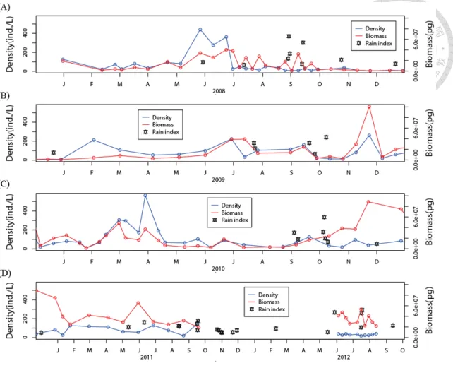
Figure 10 Time series of total zooplankton density and biomass for (A) 2008, (B) 2009, (C) 2010, (D) 2011 and 2012. The red and blue lines represent discharge and precipitations respectively. The black stars indicate EP events, with its y-axis position indicating the relative extent of precipitation.

(55)

47

Figure 11 Time series of percentages of the four zooplankton groups in terms of (A) density and (B) biomass. The red, green, blue, and black lines represent Cyclopoida, Calanoida, Cladocera, and Rotifer, respectively. The black stars indicate the precipitations of EP events.

(56)

48

Figure 12 Scatter plots illustrating the relationship in change percentage of the total density and biomass of zooplankton between two consecutive samplings. The data are classified according to (A) seasons and (B) typhoon, extreme rain, and normal days.

The horizontal and vertical black lines indicate a 0 % change.

(57)

49

Figure 13 Change percentage of total density and biomass of zooplankton between two consecutive samplings in different stages of extreme precipitation events (A) and size composition in terms of density (B) and biomass (C). For (A), the vertical bar represents the standard error. For (B) and (C), the total height is 100 %, and the colors represent different size classes. From left to right, bars represent the pre-EP (extreme precipitation) stage, the 1st week of post-EP stage, the 2nd week of post-EP stage, and so on, respectively.

(58)

50

Figure 14a Two dimension plot of canonical functions of the discriminant analysis.

This plot describes the results from density data. The red, green, blue, and yellow circles represent post-EP week 1, 2, 3, and 4, respectively. The squares, triangles, rhombus, and stars represent spring, summer, autumn, and winter respectively for normal days (i.e. not after EP events). LD represents coefficients of linear discriminants.

(59)

51

Figure 14b Two dimension plot of canonical functions of the discriminant analysis.

This plot describes results from the biomass data. The red, green, blue, and yellow circles represent post-EP week 1, 2, 3, and 4, respectively. The squares, triangles, rhombus, and stars represent spring, summer, autumn, and winter respectively for normal days (i.e. not after EP events). LD represents coefficients of linear discriminants.

(60)

52

Figure 15 The extent of dispersion of discriminate groups at different stages after extreme precipitation events and in normal days calculated based on (A) density and (B) biomass data. The between-group dispersions were assessed by Tukey's ‘Honest Significant Difference’ method. The vertical bar represents the standard error.

(61)

53

Table

Table 1 The definition of extreme precipitation and its sub-categories. The classification of typhoons and precipitations is determined according to the guide published by the Central Weather Bureau in Taiwan (CWBT) and a previous study (Tsai et al. 2011).

Extreme precipitation

Typhoon Area within typhoon radius of a typhoon determined by CWBT (by wind) passed over Feitsui Reservoir region.

Small typhoon According to classification of typhoon of CWBT.

Medium typhoon According to classification of typhoon of CWBT.

Large typhoon According to classification of typhoon of CWBT.

Extreme

rain

ADAP recorded by TFRA of a rain event is larger than 50 mm/day except typhoon.

Heavy rain ADAP>50 mm/day

Extremely heavy rain ADAP>130 mm/day

Torrential rain ADAP>250 mm/day

Extremely torrential rain ADAP>350 mm/day ADAP：Averaged daily accumulated rainfall,

TFRA：Taipei Feitsui Reservoir Administration

(62)

54

Table 2 Results of randomization tests for abiotic and biotic factors.

Environmental factors p value

Total Suspended Matter (TSM) 0.008 **

Optical Backscatter Sensor (OBS) 0.008 **

DOC 0.385

PAR 0.326

NO2 0.166

NO3 0.167

PO43- <0.001***

Total bacteria biomass 0.016 *

Chlorophyll a 0.013 *

Zooplankton Total density 0.001 **

Zooplankton Total biomass 0.001**

Significant p-values are shown in red color with the * symbol. Significant symbol: 0 <

*** < 0.001 < ** < 0.01 < * < 0.05 < . < 0.1 < < 1.

(63)

55

Table 3a Binominal tests for the response of OBS after extreme precipitations or a normal day. “Increase” and “decrease” represent the count of increase or decrease in OBS.

OBS

Increase (a) Decrease (b) Ratio (a/b) p value Typhoon

(1st post week) 10 4 2.5 0.009 **

Extreme rain

(1st post week) 18 13 1.385 0.014 *

TY recover (2nd~4th post

weeks)

10 21 0.476 0.713

ER recover (2nd~4th post

weeks)

17 24 0.708 0.516

TY + ER (all

post weeks) 55 62 0.887 0.016 *

Normal day 27 48 0.563 (as baseline)

*** < 0.001 < ** < 0.01 < * < 0.05 < . < 0.1 < < 1.

(64)

56

Table 3b Binominal tests for the response of phosphate after extreme precipitation or a normal day. “Increase” and “decrease” represents increase or decrease in phosphate.

PO43-

(1st post week) 12 3 4 0.008 **

Extreme rain

(1st post week) 19 19 1 0.625

weeks)

18 10 1.8 0.056 .

weeks)

22 32 0.688 0.586

TY + ER (all

post weeks) 71 64 1.109 0.083 .

*** < 0.001 < ** < 0.01 < * < 0.05 < . < 0.1 < < 1.

(65)

57

Table 3c Binominal tests for the response of chlorophyll a after extreme precipitation or a normal day. “Increase” and “decrease” represents the count of increase and decrease in chlorophyll.

Chlorophyll a

(1st post week) 5 9 0.556 0.594

Extreme rain

(1st post week) 10 23 0.435 0.081 .

weeks)

21 10 2.1 0.0183 *

weeks)

24 21 1.143 0.370

TY + ER (all

post weeks) 60 63 0.952 0.528

*** < 0.001 < ** < 0.01 < * < 0.05 < . < 0.1 < < 1.

(66)

58

Table 4a Species scores in discriminant analysis from density data. The species scores were calculated from LD1 and LD2 by equation 3. The top 13 ranked species whose accumulated percentage of score account for 80 % of the total species score were shown above the red line, among which those who also ranked in the top species according to the biomass data (following the same 80% threshold procedure) are indicated by bold. LD: coefficients of linear discriminants.

Density

Species Score Category Percentage of Score

Accumulated percentage Brachionus

urceolaris 35.45 Rotifer 34.96 34.96

Conochilus

unicoruis 18.98 Rotifer 6.92 41.89

Collotheca

mutabilis 13.37 Rotifer 5.70 47.58

Moina

micrura 10.05 Cladocera 5.51 53.10

Mongolodiapto

mus birulai N 9.50 Copepod

nauplius 5.00 58.10

Ploesoma

hudsoni 8.84 Rotifer 3.98 62.08

Daphnia

cucullata 8.58 Cladocera 3.33 65.42

Conochiloides

dossuarius 8.16 Rotifer 2.93 68.35

Diurella

stylata 7.46 Rotifer 2.82 71.17

Trichocerca

capucina 7.43 Rotifer 2.51 73.67

Cyclopoida

Nauplius 6.94 Copepod

nauplius 2.48 76.16

颱風及極端降雨在翡翠水庫中經由上行效應對浮游生物的影響

國立臺灣大學理學院海洋研究所 碩士論文

National Taiwan University Master Thesis

颱風及極端降雨在翡翠水庫中經由上行效應對浮游生 物的影響

Influences of typhoons and extreme rains on plankton through bottom-up effects in Feitsui Reservoir

黃煒忠

Wei-Chung Huang

指導教授：謝志豪 博士 Advisor: Chih-hao Hsieh, Ph.D.

中華民國 104 年 7 月

July, 2015

致謝

Contents

Abstract

中文摘要

Introduction

Materials & Methods

Den = N × (F − F ) × α × r × π × 1000 ×

Data Analysis

CP ( ) =

× 100%

CP ( ) = × 100%

SS = (SS in LD1) + (SS in LD2)

Dis = 2 × ∑ ∑

Results

Discussion

Conclusion

Figure References

Table References

Figure

Table

國立臺灣大學理學院海洋研究所碩士論文

颱風及極端降雨在翡翠水庫中經由上行效應對浮游生物的影響

指導教授：謝志豪博士 Advisor: Chih-hao Hsieh, Ph.D.