Institute of Oceanography College of Science
National Taiwan University Doctoral Dissertation
Climate and fishing effects on the distribution and size structure of exploited fish populations
3 Chen-Yi Tu
Advisor: Chih-hao Hsieh, Ph.D.
107 6
June, 2018
doi:10.6342/NTU201802401
!
!
!
i!
3
3
e s
t
0
r 0
3 4
E
1 6
6 2
2
E
7
doi:10.6342/NTU201802401
!
!
!
iii!
Abstract
!
Climate and fishing effect on the exploited populations is an important research topic. Although the global meta-analysis indicates a general pattern of poleward distributional shifts in response to rising temperatures, the specific responses have varied among species. The size structure of exploited populations is simultaneously affected by both climate and fishing, but what determines the relative contribution of the two remains unknown. More importantly, the dynamics of distribution and size structure of exploited populations may be interwoven because of the ontogenetic habitat shift of fish. Therefore, a framework to incorporate these two demographic aspects is urgently needed to gain the whole picture for understanding exploitation population’s response to climate and fishing effect.
In my thesis, I use three different approaches to investigate climate and fishing effects on the distribution and size structure of the exploited fish populations. The first chapter describes the general phenomenon and set the research scene. The second chapter describes how fish with different life history traits respond differently at interannual and decadal scales of climate change, using the bottom trawl fishery in the Japan Sea as an example. The results indicate that the distributional changes of species in response to decadal climate variability are best explained by asymptotic length, which indicates that warming has greater negative effects on larger fishes in the Japan Sea. The third chapter focuses on the size structure of exploited fish population, with emphasis on applying variation partitioning to disentangle the synergetic effect of climate and fishing. The results show that fishing has the most prominent effect on the size structure of exploited stocks. In addition, the fish stocks experienced higher variability in fishing displayed a greater response to temperature in their size structure,
suggesting that fishing may elevate the sensitivity of exploited stocks in responding to environmental effects. The variation partitioning approach provides complementary information to univariate size-based indicators in analyzing size structure. The fourth chapter examines how the change in spatial distribution at different life stages is affected by climate change in exploited fish populations. I found adult stage generally move faster as response to temperature change than juvenile stages. Also, the species whose adults and juveniles move toward the same direction are more likely to have more overlapping in distribution among the two life stages, indicating that adults and juveniles of given species occupying similar niches are more likely to have similar response.
Overall, this study concludes that size structure and distribution are related in the response of the exploited population to climate and fishing effects. It would be necessary to examine both for a better understanding the responses of exploited populations. These results may provide useful information for ecosystem-based fisheries management in light of climate change.
Keywords: climate change, spatial distribution, size structure, fishing effect, life history traits
doi:10.6342/NTU201802401
!
!
!
v!
Table of Content
Chapter 1 Introduction ... 1
Chapter 2 Climate effect on species distribution: case study in Japan Sea ... 6
Introduction ... 6
Material and methods ... 7
Result ... 12
Discussion ... 13
Conclusion ... 16
Chapter 3 Fishing and temperature effects on the size structure of exploited fish stocks ... 25
Introduction ... 25
Material and methods ... 30
Results and Discussion ... 35
Conclusion ... 37
Chapter 4 Stage dependency in species distribution as response to climate change ... 47
Introduction ... 47
Material and method ... 49
Result ... 51
Discussion ... 52
Conclusion ... 54
Chapter 5 Conclusion ... 62
References ... 64
Appendices ... 75
I. Fishing effort of Japan Sea single trawl fisheries, 1972-2002 ... 75
II. Data source, map in variation partitioning analysis ... 77
List of Figures
Figure 2-1 An example map in 1972 showing the spatial distribution of CPUE (kg/haul) for Pacific cod (Gadus macrocephalus) calculated from the Japan Sea Offshore Bottom Trawl dataset during spawning season.!...!22!
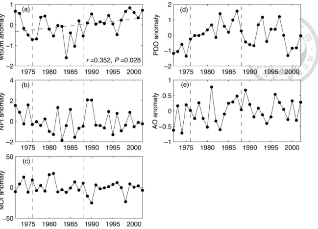
Figure 2-2 Annual anomalies time series of the environmental variables. The vertical dash lines indicate the duration of cold (1977/78-1988/89) period based on PDO and NPI (Hare and Mantua, 2002). The trend lines (dash line) and correlation coefficients are shown in the time series when a significant long-term trend
(P<0.05) exists.!...!23!
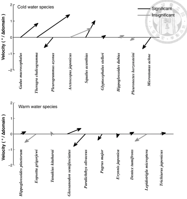
Figure 2-3 Summaries of the movement from the cold to the warm period (∆ domain).
The y-axis denotes the unit of velocity for the arrow vectors in the vertical direction, with 1° ≈ 111.2 km. The significant distributional shifts passed the randomization test (see text) were shown in black line.!...!24!
Figure 3-1 Boxplot shows the variation of size structure explained by the fishing, temperature, and interactive effect. Results of ANOVA indicate that the fraction of variation explained by fishing is significantly higher than the temperature
(P=0.019) and interactive effect (P<0.001), but fraction of variation explained by temperature is not significantly different from interaction (P=0.344).!...!42!
Figure 3-2 Boxplot shows the variation of size structure explained by the fishing, temperature, and interactive effect grouped by areas. Fraction of variation explained by fishing is significantly different from both temperature (P= 0.005) and interaction (P<0.001) in West US.!...!43!
Figure 3-3 Boxplot shows the variation of size structure explained by the fishing, temperature, and interactive effect grouped by the habitat of species. Particularly, fraction of variation explained by fishing is significantly different from both
temperature (P=0.0014) and interaction (P<0.001) for demersal species.!...!44!
Figure 3-4 Explained variation by temperature in relation to the mean and CV of mortality ratio or temperature. The line is the best-fitted regression line based on the linear mixed effect model with each fishing/temperature index as fixed effect and habitat as random effect. The solid line indicates the significant result (d).!....!45!
doi:10.6342/NTU201802401
!
!
!
vii!
Figure 3-5 Comparison of P values of (a) fishing and (b) temperature effect estimated from the variation partitioning approach versus univariate SBIs. The diagonal line represents the 1:1 line. Results of binomial test indicate that variation partitioning is more efficient in rejecting the null hypothesis (p-value is smaller) than the univariate SBIs in detecting temperature effects (Probability of success=0.63, P=0.003) and marginally in fishing effects (Probability of success=0.56, P=0.10)
!...!46!
Figure 4-1 An example map showing of centroid changes through time
(1991Q1-2014Q3) for adult (red) and juvenile (blue) stages using Atlantic cod.!..!57!
Figure 4-2 Box plot summarizing moving speed (absolute value of b1 in latitude ~ b1* temperature +b0) as response of temperature for the adult and juvenile stages. Only the species found a significant relationship with temperature were included. The Mann-Whitney U test indicates significant difference (P=0.036) between two stages.!...!58!
Figure 4-3 Box plot of summarizing moving speed (absolute value of b1 in latitude ~ b1* temperature +b0) as response of temperature for the different catch type and biogeographic groups. Only the species at given stage found a significant
relationship with temperature were included. The Mann-Whitney U test indicates no significant difference between two catch types in adult stage (a) and
biogeographic groups (b).!...!59!
Figure 4-4 Feather plots for each species show the how moving direction of centroid varies through time. The red arrows denote adult stage, while the blue arrows denote juvenile stage.!...!60!
Figure 4-5 Relationship between ratio of overlapped area and correlation of moving direction between adult and juvenile stages. Species with high proportion of
overlapped area are more likely to move in the same direction (R2=0.46).!...!61!
List of Tables
!
!
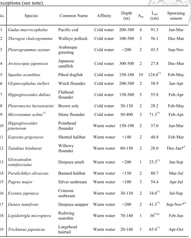
Table 2-1 Life history traits (age at maturation Am and asymptotic length Linf) and geographical affinity of the target species in the Japan Sea single-trawl fisheries (Tian et al., 2011). The asymptotic lengths are mostly compiled from Ogata (1980) with some exceptions (see note). ... 17 Table 2-2 Correlation matrix of environmental variables ... 18 Table 2-3 Results of regression analyses investigating the effects of interannual changes
in environmental variables on median latitude and longitude and boundary (minimum latitude/ longitude for cold water species and maximum latitude/
longitude for warm water species, respectively). The decadal changes between two domains (cold-warm) are also shown here. ... 19 Table 2-4 Results of logistic regression (logit(y) ~ β0 +β1x) investigating effects of
geographical affinity and life history traits (x) on species' response (y) to climate variations at interannual (latitude and longitude are shown separately in (a) Distribution) and decadal scale. The AIC intercept (β0), and regression coefficient (β1) values with significance in the Rao’s score test (P < 0.05) are in bold font. .. 20 Table 2-5 Average abundance (kg/haul) in the cold and warm period and results of
regression analyses linking the environmental variables with abundances. ... 21 Table 3-1 Data regions and periods for the 28 commercial stocks. The abbreviation in
the bracket indicates the location of stock: AI, Aleutian Islands; EBS, East Bering Sea; GOA, Gulf of Alaska. ... 39 Table 3-2 Results of variation partitioning showing the relative contribution of fishing,
temperature, and their interactive effect to the total variation (in term of adjusted R2 value) for each of the 28 stocks ... 40 Table 3-3 Results of univariate linear regression analysis on % variation explained by
fishing or temperature versus each life history trait, mean mortality ratio
(meanF_M), CV of mortality ratio (cvF_M)), mean temperature (meanTemp), and CV of temperature (cvTemp) ... 41 Table 4-1 Species used in analysis. The trophic level and biogeography is from Yang
(1982) and the juvenile length is obtain from ICES FishMap. ... 55
doi:10.6342/NTU201802401
!
!
!
ix!
Table 4-2 Regression coefficient on latitudinal shift of centroid to temperature in two stages (badult and bjuvenile) and the correlation coefficient of moving direction (θ, angle) between adult and juvenile stages for each species, respectively. The
overlap ratio is the ratio of overlapped area divided by the full-occupied area. .... 56
Chapter 1 Introduction
Climate and fishing are two major driving forces for the variability of fisheries resources (Perry et al. 2005). Accumulating evidence demonstrates the effects of climate on the spatial distribution, abundance, size structure and phenology of populations (Stenseth et al. 2002, Parmesan and Yohe 2003, Ottersen et al. 2010, Walther 2010, Doney et al. 2012, Cheung et al. 2013b). Interestingly, recent meta-analyses indicated that the rates of the observed shifts in the distribution and phenology of marine species are comparable to or greater than those of terrestrial systems, which may be due to an area of high velocity (movement of isotherm over year) extending across broader regions in the ocean than land (Burrows et al. 2011) or the greater dispersal facilitated by circulation in the marine environment (Poloczanska et al.
2013).
For fishes, climate effect on spatial distributions of fishes is well documented (Perry et al. 2005, Dulvy et al. 2008, Hsieh et al. 2008a, Mueter and Litzow 2008, Hsieh et al. 2009b, Nye et al. 2009, Engelhard et al. 2011, Keller et al. 2013, Pinsky et al.
2013, Bell et al. 2015). These changes of spatial distribution are not random, as the abundance-occupancy relationship described by meta-population theory and the density-dependent habitat selection (DDHS). Based on DDHS, species may occupy the distinctive patches or optimal habitat first (MacCall 1990). Hence, climate-induced reorganization of communities may have ecosystem consequences that could cause changes in fisheries production (MacNeil et al. 2010, Hollowed et al. 2013). Such relationship between abundance and spatial distribution also imply that change in spatial distribution may further impact the population abundance and eventually persistence
doi:10.6342/NTU201802401
!
!
!
2!
(Hsieh et al. 2010a).
In addition to distribution, climate effects on size structure of population (Daufresne et al. 2009a) also receive much attention. Warming can cause size structure shrink toward smaller size (Cheung et al. 2013a). This may be due to the metabolism at individual levels (Gillooly et al. 2001a), which increases growth rate and causes earlier maturation at population level (Neuheimer and Grønkjær 2012). Besides metabolic mechanism, warming may indirectly affect the population structure through the recruitment process that increases the proportion of juvenile in the whole populations (Sundby 2000).
Furthermore, the responses of species to climate variability can vary greatly (Chen et al. 2011), even within the same ecosystem (Hsieh et al. 2005, Perry et al. 2005, Tian et al. 2008, Hsieh et al. 2009a, Nye et al. 2009). Some studies link the species response with life history traits. In the North Sea study, species with a short life span and small body size were more likely to shift poleward as a result of warming (Perry et al. 2005).
However, some studies suggest that the distributional response depends on the biogeography of each species; for example, the southern and northern fish stocks of the continental shelf of Northeast U.S. have exhibited contrasting responses to recent warming (Nye et al. 2009).
However, climate and fishing effect can interweave with each other that become difficult to separate. Some evidences suggest fishing may increase the sensitivity of exploited populations to climate variability (Hsieh et al. 2006a). Fishing is a process of size-selective removal of larger individuals, which may truncates the population structure toward smaller size. There are three consequences at the population levels that may due to fishing: change of the size structure that reduces the buffering capacity of the population (Hsieh et al. 2006a); reduced spatial homogeneity in exploited species
(Hsieh et al. 2008b) or removal of spatial-subunits that results in increasing overall population sensitivity to climate fluctuation at interannual to multi-decadal scales (Ottersen et al. 2006); and alteration of life-history traits (de Roos et al. 2006).
Although a growing number of studies have tried to investigate the synergetic effect of climate and fishing, the relative contribution of changing species spatial distribution and size structure remains poorly understood.
It is also known that species spatial distribution and size structure are not two independent characteristics. Individuals at different life stages may migrate into different habitats, or part of the habitats, is often referred as ontogenetic habitat migration. This provides multiple possible ways for climate to affect individual species as they grow and mature (Rijnsdorp et al. 2009, Petitgas et al. 2013). Although previous studies suggest ontogenetic migration of marine species is common (Wilbur 1980, Gibson et al. 2002, Kotwicki et al. 2005, Hoff 2008), many of the studies focused on specific habitat (Dahlgren and Eggleston 2000) and only limited studies focused on exploited species (Barbeaux and Hollowed 2018).
To investigate climate and fishing effects on the distribution and size structure of the exploited fish populations, a more complex, thorough approach is necessary. In this thesis, I try to investigate the effects from three different approaches: climate effect on spatial distribution of species with different life history traits; climate and fishing effects on size structure of exploited species; and climate effect on the distribution of exploited and unexploited species at different life stages. The second chapter describes how fish with different life history traits respond at interannual and decadal scales of climate change, using the bottom trawl fishery in the Japan Sea as a case study. The results indicate that the distributional changes of species in response to decadal climate variability are best explained by asymptotic length, indicating that warming has greater
doi:10.6342/NTU201802401
!
!
!
4!
negative effects on larger fishes in the Japan Sea.
The third chapter focuses on the size structure of exploited fish population, with emphasis on applying variation partitioning to disentangle the synergetic effect of climate and fishing. By applying the variation partitioning to the size structure data, the results show that fishing has the most prominent effect on the size structure of exploited stocks. In addition, the fish stocks experienced higher variability in fishing have a greater response to temperature in their size structure. This may suggest that fishing may elevate the sensitivity of exploited stocks in responding to environmental effects.
This variation partitioning approach, which provides complementary information to univariate SBIs in analyzing size structure, may provide insight for ecosystem-based fisheries management
In the fourth chapter, I examine how the change in species distribution at different life stages is affected by climate change in exploited fish populations. I used International Bottom Trawl Survey at North Sea as an example and divided each species into two subgroups based on their size: juvenile and adult. I found adult stage generally move faster as response to temperature change than juvenile stages. Also, the species whose adults and juveniles move toward the same direction are more likely to have more overlapping in distribution among the two life stages, indicating that adults and juveniles of given species occupying similar niches are more likely to have similar response. The results may have further implications for studies on population level responses, namely that ontogenetic differences should be taken into consideration when assessing the impacts.
Overall, this study concludes that size structure and distribution are both important for understanding the responses of exploited populations to climate and fishing effects.
These results may provide useful information for ecosystem-based fisheries
management in light of climate change.
doi:10.6342/NTU201802401
!
!
!
6!
Chapter 2 Climate effect on species distribution: case study in Japan Sea
(This chapter is originally published as: Tu, C.-Y., Tian, Y., & Hsieh, C.-H. (2015).
Effects of climate on temporal variation in the abundance and distribution of the demersal fish assemblage in the Tsushima Warm Current region of the Japan Sea.
Fisheries Oceanography, 24(2), 177–189. http://doi.org/10.1111/fog.12101.)
Introduction
To demonstrate the climate effect on species distributional response, I looked into the demersal fish assemblage of the Tsushima current region of Japan Sea. The data we analyzed comprised the catches and efforts of the Japanese single-trawling fishery, which were derived from the Japan Sea Offshore Bottom Trawl fisheries dataset (JSOBT). Because of the wide-coverage and the target species vary in their geographical affinities and life history traits (Table 2-1), the single trawling data may provide a unique opportunity to examine how the biological characteristics of species influence their response to climate variability.
Previous studies of the ecosystem response to climate variability in the Japan Sea found possible relationships between climate and biological populations (see the summary in Chiba et al. (2008)). The Japan Sea is a semi-enclosed sea, thus the seasonal and interannual variations in its hydrography are presumably affected by basin-scale climatological events (Naganuma 2000, Watanabe et al. 2003). The 1976/77 shift in the plankton biomass in the Japan Sea ecosystem coincided with the Pacific Decadal Oscillation (Chiba and Saino 2002, Chiba et al. 2005). This change to a lower trophic level might have been transferred to upper trophic levels because the
abundances of fishes also exhibited similar decadal variability. A more recent study found that different pattern of abundance fluctuated between the cold- and warm-water species during the regime shift in the late 1980s (Tian et al. 2011), with indicates the importance of the geographical affinity of fishes in response to environmental forcing.
However, most of these studies only focused on changes in abundance. Thus, the climate-driven changes in the geographical distributions of the biological population at interannual and decadal scales are unclear. The geographical distributions of some demersal species appear to reflect the decadal variability in climate (Tian et al. 2008), but no systematic studies have investigated the distributional responses of demersal species at interannual and decadal scales. In addition, the relationships of these responses to the ecological and life history traits of demersal species remain elusive.
In this chapter, I assessed the environmental variability in the Tsushima Current region of the Japan Sea based on local- and basin-scale environmental indicators. I also investigated whether the changes in distribution and abundance were significant at interannual (1972–2002) and decadal scales [between the cold (1977–1988) and warm (1989–2002) periods]. Finally, I determined how well the geographic affinity and life history traits could explain the sensitivity of the responses of species. I anticipated that this approach based on using two temporal scales to assess changes in geographical distribution and abundance would elucidate how demersal fishes have responded to environmental variation in the Japan Sea ecosystem.
Material and methods Fisheries data
To examine the effects of climate on the abundances and distributions of demersal species, I studied 19 species from the fisheries targets that underwent single trawling
doi:10.6342/NTU201802401
!
!
!
8!
during 1972-2002 based on the JSOBT dataset (Misu 1974, Tian et al. 2008, Tian et al.
2011). For further analysis on life history effect and data consistency, I excluded species recorded as a group and the data in offshore area owing to the limited species and discontinuous records in space and time. To generate the distribution map for each month for each species, I summed up the catch and effort in each fishing area (the smallest unit in record is 10’ x 10’ grid) and calculated the catches per united effort (CPUE) by dividing the total catches by the total efforts (number of hauls) in the grid.
In following analysis, I only consider the spawning season of each species because climate variability acting at the ocean surface is more likely to affect demersal species during their spawning (Minami and Tanaka 1992, Rijnsdorp et al. 2009). I used the spatial data averaged across the spawning period to produce the annual map.
For the indices of spatial distribution to each species, I calculated CPUE-weighted median latitude and longitude as the distribution center for each species using annual CPUE map, and a time series for the distribution center for each species was obtained.
In addition, the southern and northern boundaries were calculated as the minimum and maximum latitudes, respectively, where a species occurred on the annual CPUE map.
Similarly, the eastern and western boundaries were calculated as the maximum and minimum longitudes, respectively.
Environmental variables
To understand the effects of climate on the Japan Sea ecosystem, I examined local- and basin-scale climate indicators. The local-scale indicator was the 50-meter depth water temperature (wt50m) in the Tsushima Current region. The basin-scale climate indices comprised the Pacific Decadal Oscillation (PDO; Mantua and Hare (2002)), Arctic Oscillation (AO, Thompson and Wallace (1998)), North Pacific Index (NPI,
Trenberth and Hurrell (1994)) and Asian Monsoon Index (MOI, (Hanawa et al. 1988, Watanabe et al. 2003)). In the analysis of the environmental data, I only used the quarterly data that corresponded to the fishery data.
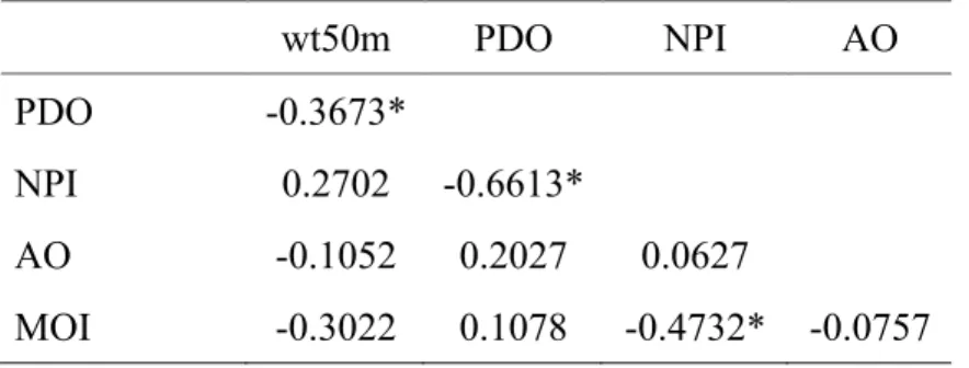
The correlation analysis between the local- and basin-scale climate indicators detected a complex interaction between atmospheric forcing and local water temperature (Fig. 2-2, Table 2-2).
Analysis of environmental effects on the demersal species
To understand the effects of climate on the demersal species, I analyzed the shifts in distribution and abundance separately at both interannual and decadal scales, I used the analytical framework reported by Hsieh et al. (2009b), and outlines of the procedures are given as follows. I defined the cold (1977–1988) and warm (1989–2002) periods based on previous studies of the decadal variability in the Japan Sea ecosystem (Chiba and Saino 2002, Chiba et al. 2005, Tian et al. 2008). In the decadal analyses, I excluded data obtained before 1976 because previous studies (Chiba and Saino 2002, Chiba et al. 2005, Tian et al. 2008) suggest that a decadal shift occurred in 1976/77. In addition, the data period (1972–1976) was too short to make quantitative comparisons.
Thus, I focused on the decadal event. The temperature anomalies suggested that a minor warming may have occurred prior to 1976, but it is likely to have been part of fluctuations on a shorter time scale in the Japan Sea rather than a decadal event (Katoh et al. 2006).
To examine the distributional response at the interannual scale, I performed regression analysis of the environmental variables and distribution center (median latitude/longitude) for each species. I also investigated 1-year and 3-year time-lagged values that represented the delayed environmental effects, which have been observed in
doi:10.6342/NTU201802401
!
!
!
10!
fish species in the North Sea (Perry et al. 2005) and southern California region (Hsieh et al. 2008a). To account for the serial dependency of the time series in regression analyses, I calculated the regression coefficient using the estimated generalized least square (EGLS) method and computed the bootstrapped (1000 times) 95% confidence limits for the hypothesis test (Ives and Zhu 2006). In addition, I examined the boundary of the distribution relative to the environmental variables. I only examined the minimum latitude (5th percentiles) as the southern boundary for cold water species and the maximum latitude (95th percentiles) as the northern boundary for warm water species, respectively, because the Japan Sea is near the southern most limit for most of the cold water species and the northernmost limit for warm water species. In addition, the dynamics at the range boundaries (latitudinal and elevation in terrestrial ecosystem) are expected to be more sensitive to climate variability (Parmesan and Yohe 2003). For the longitudinal boundary, both the minimum and maximum longitudes (with the same calculation as in latitudinal boundaries) were used in analysis. I included abundance in the analysis and examined the partial correlations between the distribution center (or boundary) and environmental variables if a species’ distribution center (or boundary) was significantly correlated with abundance (P < 0.05), because the geographical extent of marine populations may be correlated with their population size (MacCall 1990, Hsieh et al. 2010a). The aim was to separate the possibility that the distributional shift was caused solely by expansion/constriction due to changes in population size.
However, our results were qualitatively the same when abundance was not included as a covariate. For the time series regression analyses, I set the significance level at 5%, without correcting for multiple tests. My analyses aimed to explore potential climate effects, but various climate indices are correlated (Table 2) thus different tests should not be considered to be independent.
At the decadal scale, to examine the change in the geographical distribution of each taxon from the cold to warm period, I estimated the centroid for each period based on the time series of the distribution centers (the median latitude and longitude were considered simultaneously) by 50% convex-hull peeling (Zani et al. 1998), where all of the distribution centers were weighted equally. This method is robust to the bias caused by potential outliers. I then tracked the movement direction and magnitude of each species from the cold to warm period to determine the decadal variation in the distribution centers. Finally, I used an ANOVA-like randomization test (Hsieh et al.
2008a) to examine whether the shift in centroids between the cold and warm periods was statistically significant for each species.
I then considered whether differences in geographic affinity and life history traits existed between geographically shifting and non-shifting species. I defined the
“geographically shifting species” as those species that exhibited significant distributional shifts at interannual or decadal scales (changes in their distributional domain from the cold to the warm period). For the interannual scale, I analyzed the latitudinal and longitudinal shifts separately. The “geographical affinity” was defined as the cold or warm water group (see Table 2-1) based on studies of a species’
biogeography (Nishimura 1968). The life history traits comprised age at maturation (Am) and asymptotic length (Linf) because these traits were available for all of the species examined. Univariate and multivariate logistic regressions (the latter with stepwise forward selection based on AIC) were used to determine factors that are able to classify the different responses (shift or non-shift) in geographical distributions. The goodness-of-fit was evaluated by AIC, and then Rao's score test (Rao 1948) was used to test whether the value of regression coefficient is significant. Rao test is asymptotically equivalent to the likelihood ratio and Wald test, but it is known to be useful for testing
doi:10.6342/NTU201802401
!
!
!
12!
the improvement of model fit if variables that are currently omitted are added to the model. Therefore, Rao test is often recommended for identifying variable in stepwise forward selection.
Result
The interannual variations in the distribution centers of the demersal species were largely related to environmental variables (Table 2-3). The median latitude and longitude were correlated with environmental variables for more than half of the species, and a limited number of species exhibited distributional shifts only in their boundaries.
The rate of latitudinal shift (center) ranged from –54 to 44 km/°C with an overall average of 5.110 ± 6.617 (standard error) km/°C. Similarly, the longitudinal shift (center) ranged from -45 to 52 km/°C with an overall average of 6.281 ± 6.565 (standard error) km/°C.
Approximately 68% of the species exhibited a significant distributional shift from the cold to the warm period at the decadal scale (Table 2-3), but the movement direction varied among species (Figure 3). Four species in the cold water group exhibited significant poleward shifts, particularly Gadus macrocephalus, Theragra chalcogramma, and Squalus acanthias (Figure 2-3). However, these poleward shifts did not prevail in warm water species. The most significant poleward shift occurred in Glossaodon semifasciatus, whereas Paralichthys olivaceus, Pagrus major, and Evynnis japonica exhibited significant equatorward shifts among the warm water species (Figure 2-3b).
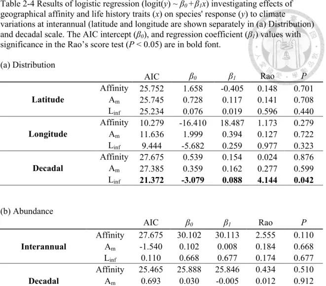
The results of the logistic regression showed that none of the variables we examined (life history traits and geographical affinity) could classify the different distributional responses (shifting v.s. nonshifting) among the species at the interannual
scale (Table 2-4a). At decadal scale, the Linf was significant (P = 0.042) for classifying the distributional responses among the species (Table 2-4a). The results of the multivariate logistic regression were quantitatively the same as the univariate analysis results; thus, only the latter are shown.
Discussion
In this study, I examined the changes in the geographical distribution of the demersal fish assemblage in the Japan Sea and found significant effects of climate. The responses in the distribution in terms of latitudinal and longitudinal shifts at the interannual scale were found in both the cold water and warm water groups. The configuration of the narrow continental shelf in the Japan Sea runs from the northeast to the southwest (Figure 2-1), which may suggest that the overall trend in the along-shore movement is related to environmental variability. However, the rate of distributional shift in the Japan Sea was smaller than that found in a previous study (Poloczanska et al.
2013) and it exhibited a high variance. This also suggests that the universal poleward shift detected by a global-scale meta-analysis might not hold at the regional scale (see Perry et al. (2005)). One may argue that a deepening of the vertical distribution is a more universal response to warming than a latitudinal shift for demersal fishes (Dulvy et al., 2008); however, the demersal fishes surveyed during the warming period did not reveal evidence of deepening in the Japan Sea (Kawamura 2009).
The distributional shifts at the decadal scale also exhibited along-shore movement, but the scales varied among different species (Figure 2-3). In contrast to a previous study (Perry et al., 2005), I found that species with a large body size (Linf) were more likely to respond by changing their distribution (Table 2-4). It is unclear why I reached the opposite conclusion, but Morita et al. (2010) provided a possible explanation. Using
doi:10.6342/NTU201802401
!
!
!
14!
a simple bioenergetic model, they showed that the optimal temperature for growth decreases with increasing body size, which indicates that species with large body sizes may be more vulnerable to warming. It is also possible that fishing may affect the species distributional response to climate change. The large species in the Japan Sea, such as G. macrocephalus, S. acanthias, and P. olivaceus, are important targets of fisheries, thus these large species may experience a higher rate of exploitation than other species. These effects of fishing on the spatial distribution of marine fish were also found in the California Current region, where the exploited species were more sensitive to warming (Hsieh et al. 2008a).
I observed variations in the distributional shift among species at both interannual and decadal scales. It is possible that the different physiological requirement of species or even multiple stocks within one species may have restricted their distribution. In the Japan Sea, Arctoscopus japonicus and P. olivaceus are known to comprise two separate stocks. For A. japonicus, the recent catch statistics for all fisheries combined suggest that the northern stock has been depleted since 1980 (Fujiwara et al. 2009) whereas the southern stock remains relatively stable (Matsukura et al. 2014). Similarly, the northern stock of P. olivaceus was listed as unsustainable in a recent stock assessment report (Uehara et al. 2014) whereas the southern stock was listed as sustainable (Nakagawa et al. 2014). This north–south difference may explain the southeastward movement of P.
olivaceus, as shown in Figure 3. In addition to the presence of multiple stocks of certain species in the Japan Sea, other fisheries such as small-scale trawling in the coastal area of Kyoto Prefecture also target the single-trawling species. This multi-fisheries scenario may generate regional differences among species and stocks. These regional differences could also indicate differences in the responses to climate or fishing.
In addition, several other processes can generate various responses in the
distributional shift among species (Chen et al. 2011, Hollowed et al. 2013). In addition to environmental factors and primary production, which are often linked with the recruitment success (e.g., Beaugrand et al. (2003a)), species interactions (e.g.
competition and predation) may also play roles in mediating the response to climate change. For flatfish, the competition for habitat can affect the success of recruitment during the post-larval stages. Some studies indicate that the quantity of available habitat is crucial for juvenile settlement and it also affects recruitment (Gibson 1994, van der Veer et al. 2000). Thus, interspecific density dependence (Hixon and Jones 2005) may become important when suitable habitats are limited. For demersal species in the Japan Sea, predation or cannibalism by adult individuals may also contribute to the mortality during the juvenile stages and affect recruitment (Minami 1986, Tominaga and Nashida 1991). In these conditions, climate is not the only driving force that affects the distributions of species. It would be interesting to investigate how these biotic processes mediate the distributional responses of species to climate variability.
The use of a CPUE map to infer the distributions of species may be one of the limitations of our analyses. The fishing effort distribution for single trawl fisheries remained consistent in space and time (see Appendix I), but it is widely known that the fleet dynamics and fishermen-related factors can also affect the CPUE pattern (Branch et al. 2006). It might be possible to examine the fleet dynamics to approximate the behavior of fishermen as a Levy flight process, which is a stochastic process that is used commonly to study the foraging behavior of predators (Viswanathan et al. 1996). It is often assumed that price is the key factor that affects the behavior of fishermen, but a case study in North Sea fisheries found that the behavior of fishermen was only marginally correlated with the fish price and fishing effort (Marchal et al. 2007). A recent review also suggests that the economic factor is not the only driver of fleet
doi:10.6342/NTU201802401
!
!
!
16!
dynamics (van Putten et al. 2012). Although I neglected the influence of fleet dynamics on the fishing effort and CPUE in the present study, this issue may be addressed in future studies.
Conclusion
In this study, I provide quantitative evidence of shifts in the distributions and abundances of the demersal fish assemblage in the Japan Sea in response to climate variation. The decadal variations in distributions were explained largely by the asymptotic length, which may suggest that warming has greater negative effects on larger fishes, thereby indicating the possible effects of fishing activities. Not every kind of responses can be classified by life history traits or geographical affinity in our study.
Thus, my findings support previous studies, which showed that life history traits or geographical affinity alone, are not sufficient for interpreting the responses of species to climate variation (Hsieh et al. 2008a, Hsieh et al. 2009b). Furthermore, it would be difficult to project the responses of species to future climate change based on any single factor. More studies of the interactions among species and the biological nonlinear amplification of environmental effects will be necessary to obtain a better understanding of the effects of climate on marine ecosystems.
Table 2-1 Life history traits (age at maturation Am and asymptotic length Linf) and geographical affinity of the target species in the Japan Sea single-trawl fisheries (Tian et al., 2011). The asymptotic lengths are mostly compiled from Ogata (1980) with some exceptions (see note).
*1 FishBase (Froese and Pauly 2013)
*2 It is the main species of "other cold water flounders" (Pleuronectidae spp.) group from JSOBT dataset as in Tian et al. (2011)
*3 Narimatsu et al. (2007)
*4 Also spawn during March-May, but the peak of CPUE is in September-November.
*5 Use maximum length to represent asymptotic length because Linf is unavailable.
*6 Fujioka et al. (1990)
No. Species Common Name Affinity Depth
(m) Am Linf (cm)
Spawning season
1 Gadus macrocephalus Pacific cod Cold water 200-300 4 91.3 Jan-Mar 2 Theragra chalcogramma Walleye pollock Cold water 100-500 3 56.1 Dec-Mar
3 Pleurogrammus azonus Arabasque
greening Cold water <200 2 43.5 Sep-Nov
4 Arctoscopus japonicus Japanese
sandfish Cold water 300-500 2 27.8 Dec-Mar 5 Squalus acanthias Piked dogfish Cold water 150-180 10 124.0*1 Feb-May 6 Glyptocephalus stelleri Witch flounder Cold water 200-300 2 58.9 Jan-Apr
7 Hippoglossoides dubius Flathead
flounder Cold water 150-500 5 55.8 Feb-Apr 8 Pleuronectes herzensteini Brown sole Cold water 30-130 2 28.2 Feb-May 9 Microstomus achne*2 Slime flounder Cold water 50-400 3 71.5*1 Feb-Apr
10 Hippoglossoides pinetorum
Pointhead
flounder Warm water 150-190 2 37.0 Jan-Mar 11 Eopsetta grigorjewi Shotted halibut Warm water <140 2 40.8 Feb-Mar
12 Tanakius kitaharai Willowy
flounder Warm water 80-150 2 28.0 Dec-Jan*3
13 Glossanodon
semifasciatus Deepsea smelt Warm water <200 1 25.5*1 Jan-Sep 14 Paralichthys olivaceus Bastard halibut Warm water <150 2 80.7 Mar-Jul 15 Pagrus major Silver seabream Warm water <100 3 54.4 Apr-Jul
16 Evynnis japonica Crimson
seabream Warm water 30-130 2 34.0*1 Jul-Sep 17 Dentex tumifrons Deepsea snapper Warm water <200 2 41.5*1 Sep-Nov*4
18 Lepidotrigla microptera Redwing
searobin Warm water 70-140 1 30*5,6 Feb-Jun
19 Trichiurus japonicus Largehead
hairtail Warm water 20-140 1 65.8*1 Apr-Oct
doi:10.6342/NTU201802401
!
!
!
18!
Table 2-2 Correlation matrix of environmental variables
!
* Indicates a significant correlation (P <0.05).
wt50m PDO NPI AO
PDO -0.3673*
NPI 0.2702 -0.6613*
AO -0.1052 0.2027 0.0627
MOI -0.3022 0.1078 -0.4732* -0.0757
Table 2-3 Results of regression analyses investigating the effects of interannual changes in environmental variables on median latitude and longitude and boundary (minimum latitude/ longitude for cold water species and maximum latitude/ longitude for warm water species, respectively). The decadal changes between two domains (cold-warm) are also shown here.
A +/- sign along with the environmental variable represents significant positive/negative correlation (P<0.05). The number in the bracket indicates the lag-year with a significant correlation. For the analyses concerning boundary, "†" indicates a significant correlation in maximum boundary and the other
unmarked variables indicates a significant correlation in minimum boundary.
For the decadal shift ("shift in domain"), “+” represents a significant (P<0.05) shift from the cold (1977-1988) to the warm (1989-2002) period.
Species Median
latitude
Latitudinal boundary
Median longitude
Longitudinal boundary
Shift in domain
Gadus macrocephalus +wt50m(1) +wt50m(1) +
Theragra chalcogramma +MOI +wt50m
+AO(0, 1) +
Pleurogrammus azonus +
Arctoscopus japonicus +MOI(3) +wt50m(3)
+MOI(3) +PDO(3) Squalus acanthias +wt50m
+AO +MOI
+wt50m (0, 1) +wt50m
+AO +
Glyptocephalus stelleri +wt50m +AO(3) +
Hippoglossoides dubius Pleuronectes herzensteini
Microstomus achne +wt50m +PDO +wt50m -PDO +
Hippoglossoides pinetorum +PDO(1)† +
Eopsetta grigorjewi +wt50m(1)
Tanakius kitaharai +NPI(1) +PDO(0, 1)†
Glossanodon semifasciatus +AO(0, 1) †
+NPI(1) † +MOI(1) †
+
Paralichthys olivaceus +NPI(1) +AO(1)
+wt50m(1) +AO(1) +MOI(3)
+
Pagrus major +wt50m(0, 1) +NPI(3) +
Evynnis japonica +
Dentex tumifrons +NPI(1) +AO(1)
+PDO(3) +NPI(3) +AO(3)
+
Lepidotrigla microptera +NPI(0, 3) +MOI(3)
+wt50m(1) +NPI(3)
Trichiurus japonicus +
doi:10.6342/NTU201802401
!
!
!
20!
Table 2-4 Results of logistic regression (logit(y) ~ β0 +β1x) investigating effects of geographical affinity and life history traits (x) on species' response (y) to climate
variations at interannual (latitude and longitude are shown separately in (a) Distribution) and decadal scale. The AIC intercept (β0), and regression coefficient (β1) values with significance in the Rao’s score test (P < 0.05) are in bold font.
(a) Distribution
(b) Abundance
AIC β0 β1 Rao P
Latitude
Affinity 25.752 1.658 -0.405 0.148 0.701 Am 25.745 0.728 0.117 0.141 0.708 Linf 25.234 0.076 0.019 0.596 0.440 Longitude
Affinity 10.279 -16.410 18.487 1.173 0.279 Am 11.636 1.999 0.394 0.127 0.722 Linf 9.444 -5.682 0.259 0.977 0.323 Decadal
Affinity 27.675 0.539 0.154 0.024 0.876 Am 27.385 0.359 0.162 0.277 0.599 Linf 21.372 -3.079 0.088 4.144 0.042
AIC β0 β1 Rao P
Interannual
Affinity 27.675 30.102 30.113 2.555 0.110 Am -1.540 0.102 0.008 0.184 0.668 Linf 0.110 0.668 0.677 0.174 0.677 Decadal
Affinity 25.465 25.888 25.846 0.434 0.510 Am 0.693 0.030 -0.005 0.012 0.912 Linf 0.510 0.912 0.813 0.056 0.813
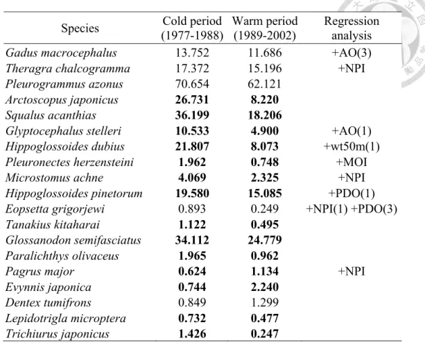
Table 2-5 Average abundance (kg/haul) in the cold and warm period and results of regression analyses linking the environmental variables with abundances.
Bold indicates a significant difference (P<0.05) of abundance between the cold and warm period. The significant positive/negative correlation (P<0.05) is indicated by a +/- sign along with the environmental variable for the regression analysis. The number in the bracket indicates the lagged year with a significant correlation.
Species Cold period
(1977-1988)
Warm period (1989-2002)
Regression analysis
Gadus macrocephalus 13.752 11.686 +AO(3)
Theragra chalcogramma 17.372 15.196 +NPI
Pleurogrammus azonus 70.654 62.121 Arctoscopus japonicus 26.731 8.220
Squalus acanthias 36.199 18.206
Glyptocephalus stelleri 10.533 4.900 +AO(1) Hippoglossoides dubius 21.807 8.073 +wt50m(1) Pleuronectes herzensteini 1.962 0.748 +MOI
Microstomus achne 4.069 2.325 +NPI
Hippoglossoides pinetorum 19.580 15.085 +PDO(1) Eopsetta grigorjewi 0.893 0.249 +NPI(1) +PDO(3)
Tanakius kitaharai 1.122 0.495
Glossanodon semifasciatus 34.112 24.779 Paralichthys olivaceus 1.965 0.962
Pagrus major 0.624 1.134 +NPI
Evynnis japonica 0.744 2.240
Dentex tumifrons 0.849 1.299
Lepidotrigla microptera 0.732 0.477 Trichiurus japonicus 1.426 0.247
doi:10.6342/NTU201802401
!
!
!
22!
!
Figure 2-1 An example map in 1972 showing the spatial distribution of CPUE (kg/haul) for Pacific cod (Gadus macrocephalus) calculated from the Japan Sea Offshore Bottom Trawl dataset during spawning season.
Figure 2-2 Annual anomalies time series of the environmental variables. The vertical dash lines indicate the duration of cold (1977/78-1988/89) period based on PDO and NPI (Hare and Mantua, 2002). The trend lines (dash line) and correlation coefficients are shown in the time series when a significant long-term trend (P<0.05) exists.
doi:10.6342/NTU201802401
!
!
!
24!
Figure 2-3 Summaries of the movement from the cold to the warm period (∆ domain).
The y-axis denotes the unit of velocity for the arrow vectors in the vertical direction, with 1° ≈ 111.2 km. The significant distributional shifts passed the randomization test (see text) were shown in black line.
Chapter 3 Fishing and temperature effects on the size structure of exploited fish stocks
Introduction
Size structure plays an important role in maintaining reproductive potential and stability of fish population. For example, larger individuals tend to produce more and better eggs (Hsieh et al. 2010b, Hixon et al. 2014) and have a longer spawning season (Berkeley and Houde 1978, Lambert 1987, Hutchings and Myers 1993, Sogard et al.
2008); small and large individuals may spawn at different sites (Trippel et al. 1997, Lawson and Rose 2000, Vandeperre and Methven 2007). Such bet-hedging strategies provide resilience capacity for populations to sustain under unfavorable conditions (Hsieh et al. 2010b, Ripa et al. 2010, Schindler et al. 2010). Hence, investigating the change of size structure may provide insight of how resilient a fish population can be.
Several external forcings may alter the size structure of a fish population. The most well-known examples are fishing and temperature. Fishing represents size-selective removal of larger individuals that can truncate the size structure of a fish population (Barnett et al. , Bianchi et al. 2000, Berkeley et al. 2004, Ginter et al. 2015), which in turn may cause recruitment failure (Ottersen et al. 2006), reduce the reproductive outputs (Scott et al. 2006), and increase variability of fish populations (Hsieh et al.
2006b, Anderson et al. 2008, Rouyer et al. 2012). It may also lead to evolutionary consequences (Heino et al. 2015); for example, the genetic differences found in the populations of Atlantic cod (Gadus morhua) from Iceland is due to difference in depth-associated fishing mortality (Jakobsdóttir et al. 2011). As such, balanced
doi:10.6342/NTU201802401
!
!
!
26!
exploitation (Law et al. 2012) and harvest-slot-limit (Gwinn et al. 2015) have been proposed to prevent fishing-induced size truncation.
Apart from fishing, increasing sea water temperature caused by global warming may also lead to shrinking size structure of marine fish populations (Daufresne et al.
2009b, Cheung et al. 2013a). Elevated ambient water temperature directly influences fish metabolism at individual level (Gillooly et al. 2001a), which increases growth rate and causes earlier maturation at population level (Neuheimer and Grønkjær 2012). Also, temperature may indirectly influence the recruitment processes through trophic transfer (Sundby 2000) and thus change the size structure. Based on the match/mismatch hypothesis, the larvae survivorship relates to the match between the timing of larval feeding and the food production (Cushing 1990). For example, rising temperature since mid-1980s has modified the plankton ecosystem and reduced the survival of young cod in the North Sea (Beaugrand et al. 2003b). While the fishing and temperature effects have been well documented, their relative contributions on the size structure of fish populations remain poorly understood. This is a critical issue particularly for exploited stocks, because overfishing has been shown to enhance the sensitivity of fish abundance and distribution to climate (Hsieh et al. 2008b, Hidalgo et al. 2011, Rouyer et al. 2014);
nevertheless, whether such synergistic effect also occurs in size structure remains relatively unexplored.
Previous studies on quantifying fishing or temperature effects on the size structure of fish populations have been focused on univariate size-based indicators (SBI). Some studies used the upper 95-percentile of the length frequency (L95) to test fishing effect (Rochet et al. 2010, Brunel and Piet 2013), while the other used length class diversity to investigate the stability of population through time (Marteinsdottir and Thorarinsson 1998). Recently, European Commission Marine Strategy Framework Directive required
regional (or local) fishery reports to provide the information of basic SBIs (e.g. the mean length) in order to improve the management and maintain the sustainable development (Farmer 2012). However, it remains unclear whether these univariate SBIs could represent the entire size structure and the status of a population. It has been suggested that no single SBI can represent an effective overall indicator for external forces (Shin et al. 2005). Also, SBIs need to be selected carefully based on their implications. For example, L95 can only reflect the variety of large fish in fish population. The analysis with the North Sea cod, herring and plaice found L95 failed to reveal the effects of external forces on fish population, as it was rather insensitive in responding to fishing mortality (Brunel and Piet 2013).
To overcome the limitation of existing SBIs, it needs an alternative approach to (1) analyze complete information of size structure and (2) examine how external forces affect the size structure. Here, I employed the variation partitioning approach to conduct a size structure-based analysis that examines the variation of size class composition in response to external forcings. Variation partitioning can be best understood as a method for extending multivariate regression. In multivariate regression (y~x), y represents a univariate response vector and x represents multiple predictors, x1, x2, etc. (each is a vector) and possibly their interactions; the contribution of each predictor variable (xi) can be evaluated by partial R-square. Whereas in variation partitioning (Y~X), Y represents a multivariate matrix and X represents multiple predictors, X1, X2, etc. (each is a matrix); the contribution of each predictor matrix (Xi) and their interaction is also evaluated by partial R-square (Peres-Neto et al. 2006). Variation partitioning is commonly used in community ecology to examine the relationship between species composition (Y matrix) and various sets of explaining variables (e.g. 2 or 3 predictor matrices) (Peres-Neto et al. 2006). This method has also been extend to analyze
doi:10.6342/NTU201802401
!
!
!
28!
temporal and space-time variation of community composition data (Griffith and Peres-Neto 2006). Here, I borrow this concept to analyze temporal variation of size composition data in responding to fishing, temperature, and the interaction, with the simplification that fishing and temperature is just a vector. Specifically, for a given fish population, I apply the variation partitioning to quantify how the temporal variation of their size composition responds to fishing, temperature and their interaction (see Methods). The explained fraction of variation (partial R-square) by each factor then allows us comparing their relative contribution in affecting length composition through time.
Next, I perform a cross-stock meta-analysis linking the relative contribution of fishing or temperature (the output of variation partitioning as explained fraction of variation) to the life history traits of fishes, as well as long-term mean and variability of fishing or temperature (see Methods). This meta-analysis aims to examine which factor can explain the relative contribution of fishing, temperature and their interaction across stocks. This meta-analysis is motivated by the fact that life history traits are associated with the size structure of population (De Roos et al. 2003). I hypothesize that the large, slow growth, and late-matured species is more likely to be impacted by fishing in their size structure because size-selective removal (i.e. size truncation) may be more severe in these species (Rouyer et al. 2011) and their recovery will take longer time (Jennings et al. 1999, De Roos et al. 2003). I also hypothesize that small species is more vulnerable to temperature effects, because smaller species are more sensitive to temperature changes due to the constrains from metabolic allometries (Gillooly et al.
2001b).
Furthermore, I expect that fishing and temperature might exhibit interactive effects via multiple ways (Perry et al. 2010, Planque et al. 2010). For example, the long-term
fishing effect, such as long-term mean and variability of mortality ratio (fishing mortality divided by natural mortality, F/M) may affect the relative contribution of temperature in explaining temporal variation of size structure. Here, I standardize fishing mortality by natural mortality in order to have a fair cross-stock comparison.
Motivated by previous studies showing that fishing elevated sensitivity of exploited stocks to environmental changes (Hsieh et al. 2006b, Anderson et al. 2008, Rouyer et al.
2011), I hypothesize that the fish stocks experienced higher fishing pressure is more responsive to temperature effect in their size structure. I also hypothesize that habitat conditions, including mean and variability of temperature, affect the relative contribution of fishing effect. For instance, Wang et al (Wang et al. 2014) found that temperature affects the cod’s life history trait, making the cod population more vulnerable to fishing.
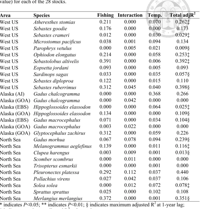
My objectives are, first, to apply variation partitioning to quantify how the variation of size structure responded to fishing, temperature and the interactive effects for 28 exploited stocks (Table 1) living in a wide range of habitats, including the west coast of US, Alaska, and North Sea (Figure S1). Secondly, I linked the fraction of explained variation by fishing (or temperature) to life history traits (including von Bertalanffy growth rate (K), length infinity (Linf), age at maturation (A50), length at maturation (L50)), as well as long-term mean and variability of fishing and habitat temperature conditions. Finally, to demonstrate the efficacy of our approach, I compared the performance of variation partitioning approach with the traditional univariate SBIs analyses. This comparison is straightforward, as both the univariate SBIs analysis and variation partitioning are computed using similar linear modeling of variance/covariance, with the difference only in the response variable- the response variable is a vector (y) in the univariate SBIs analysis whereas the response variable is a
doi:10.6342/NTU201802401
!
!
!
30!
matrix (Y) in the variation partitioning; two methods have the same explaining variables (i.e. fishing and temperature).
Material and methods
Size structure data of commercial stocks
I collected length frequency data from 28 exploited stocks, which contain temporal coverage over 20 years and annual fishing mortalities (or exploitation rates) estimated by stock assessment are available (Table 3-1, Table S1). These stocks came from 3 regions in the northern hemisphere (Figure S1): (1) the west coast of US (West US), which is part of Northeast Pacific; (2) Alaska, which separates into 3 fishing areas- Aleutian Islands (AI), Gulf of Alaska (GOA), and Bering Sea; and (3) North Sea.
Collectively, these 28 stocks in 3 regions were well studied, spanning distinct distribution of size structure, with a wide range of life-history traits and habitats, and therefore are representative of a compilation of global-scale fish stocks (Table S2).
I primarily use length frequency from the fisheries-independent surveys for each stock. These are the length frequency per size range of the given year as arranged in the stock assessment report. For Alaska region, the survey data includes bottom trawl survey in Aleutian Island (AI), East Bering Sea shelf (EBS) and Gulf of Alaska (GOA).
For the North Sea, I compiled the length frequency of ICES International Bottom Trawl Survey in the North Sea (NS-IBTS). I used the 1st quarter (Q1) in NS-IBTS for consistency because there was only annual Q1 survey prior to 1991. For the west coast of US, I used fisheries-dependent length compositions instead of bottom trawl survey because the data from fishery-independent surveys during 1980-1990 were limited.
Fishing and natural mortality
To quantify the fishing effect, I used time series of annual fishing mortality from the stock assessment reports (Supplementary Table S3-1). I focus on the single fishery whenever possible to minimize the uncertainty in fishing selectivity due to changing gears. I noted that analyses in the west coast of US use exploitation rate instead of fishing mortality in stock assessment. To make a fair comparison for meta-analysis, I transformed the exploitation rate into fishing mortality through the relationship between mortality and survival rate in fisheries (Ricker 1975). Here I first assume that these fisheries are type II fishery, in which the fishing and nature mortality operate concurrently. The exploitation rate (µ), fishing mortality (F), natural mortality (M), instantaneous total mortality rate (Z) and actual total mortality (A) have following relationships:
µ=F·A/Z (1) Z=F+M (2)
A=1-e (F+M) (3) the equation (1) can also be written as:
µ =F· (1-e (F+M))/(F+M)
With the known exploitation rate and natural mortality, this equation can be solved numerically and yields the fishing mortality. The natural mortality here is mostly compiled from the value of preferred model in the stock assessment reports (Supplementary Table S3-1, Table S3-2).
Temperature
In analysis, I primarily used empirical measurements of temperature along with the trawl surveys (see Supplementary Figure S3-2). The North Sea (53-59°N, 3°W-10°E) near-bottom temperature is the station observations of hydrochemical measurements