B3G IPv6行動網路環境之位置導向多媒體資訊服務平台---子計畫III：IPv6行動網路環境下達成比例式差別服務之頻道導向排程策略及漏失管理(I)

(1)

行政院國家科學委員會專題研究計畫成果報告

子計畫三:IPv6 行動網路環境下達成比例式差別服務之頻道導向排程策略及漏失管理(I)

計畫類別：整合型計畫

計畫編號： NSC92-2219-E-011-005-

執行期間： 92 年 08 月 01 日至 93 年 07 月 31 日執行單位：國立臺灣科技大學資訊管理系

計畫主持人：賴源正

計畫參與人員：張榮昇絲玉琴葉惠敏楊宗杰曾崇倫吳清偉

報告類型：完整報告

處理方式：本計畫可公開查詢

中華民國 93 年 12 月 8 日

(2)

中文摘要

最近幾年來在網路上提供服務品質的保證已成為一個重要的議題，比例式差別模式可提供可控制(controllable)及可預期(predicable)的服務品質，然而，目前能提供比例式差別模式的研究大都應用於有線網路，這些方法並不適用於無線網路，原因為無線網路具有高錯誤率、及頻寬會隨著行動主機位置之不同及時間的變動而有所改變。

在此報告中，我們提出兩個在無線網路上提供比例式差別模式的方法，一種針對比

例式延遲差別，另一種針對比例式產能差別。針對比例式延遲差別，我們提出Look-ahead

Waiting Time Priority(LWTP)排程器，藉由依鏈結頻寬的大小來調整傳送的順序及克服排隊領頭阻擋(HOL blocking)問題，可達到提供比例式延遲及降低佇列延遲的目的。模擬結果證實所提出的方法比之前的方法能提供較正確的延遲比例及較低的平均延遲。

針對比例式效能模型，我們提出指數規則公平性排程 (Exponential-rule Fair Queueing, EFQ)，其方法可以適用在多重狀態通道之無線網路上。EFQ 會選擇送往頻寬較高通道的資料流及落後較多的資料流，前者可降低封包的延遲，而後者可達到較佳的公平性(比例)。透過模擬的結果與 CIFQ (Channel-condition Independent Fair Queueing)比較，EFQ 能得到較低的封包延遲且更佳的公平性(比例)。

關鍵詞：比例式差別服務、服務品質保證、行動網際網路、CDMA 網路

(3)

Abstract

Providing the guarantee of the diverse Quality of Services (QoS) in the network has been an emerging issue in recent years. The Proportional Differentiated Model (PDM) was proposed to provide predictable and controllable QoS for different classes of connections.

However, most of related works focused on providing this model in a wired network. These algorithms suffer difficulty when meet some distinct characteristics, such as high error rate, location dependent or time varying channel capacity, that exist in wireless networks.

In this report, we propose two algorithms for PDM in a wireless network, one for proportional delay differentiation and the other for proportional throughput differentiation. For delay differentiation, we propose a novel scheduler to provide the proportional delay differentiation in a wireless network, in which a multi-state channel exists. This scheduler, Look-ahead Waiting-Time Priority (LWTP), can achieve proportional delay differentiation and low queueing delay, by adapting with the location-dependent capacity of a wireless link and conquering the head-of-line blocking problem. The simulation results demonstrate that the LWTP scheduler actually achieves much closer to the desired delay proportion between classes and induces smaller queueing delays, compared with the past schedulers.

For throughput differentiation, we propose a novel scheduler, Exponential-rule Fair Queueing (EFQ), for wireless fair (proportional) scheduling. Unlike current schedulers, which assume a wireless channel is just of good or bad state, EFQ aims to work with a multi-state channel. EFQ prefers the flow destined to a high-capacity channel or the flow with serious lagging. Form simulation results, EFQ not only provides shorter delay, but also achieves more appropriate fairness (proportion), compared with the Channel-condition Independent Fair Queueing (CIFQ) algorithm.

Keywords: proportional differentiated services, quality of services, mobile Internet, CDMA network.

(4)

Content

Part I

8

1. Introduction 8

2. Background 10

2.1 Proportional Differentiation Model...10

2.2 WTP...12

2.3 Problems of Scheduling over Wireless Network...12

2.4 WWTP...14

3. The LWTP Scheduler 15

4. Simulation Study 19

4.1 Packet Arrival Rate...20

4.2 Mean Channel Capacity...22

4.3 Variance of Channel Capacity...22

4.4 Number of Mobile Hosts...25

4.5 Comparison of LWTP to WWTP with a Threshold...25

5. Conclusions 28

References 29

Part II

31

1. Introduction 31

2. Background 31

2.1 Fair Scheduling Model...32

(5)

2.2 Idealized Weighted Fair Queueing (IWFQ) ...32

2.3 Channel-Condition Independent Fair Queueing (CIFQ) ...33

2.4 Exponential Rule...33

3. Exponential-rule Fair Queueing 34

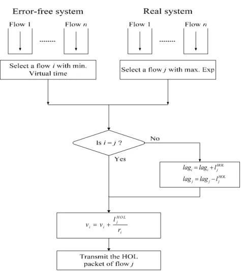
3.1 Algorithm Description...34

4. Evaluation and Discussion 36

4.1 The behavior of EFQ and CIFQ...38

4.2 Short Timescale...41

4.3 Packet Arrival Rate...42

4.4 Channel Transition Rate...45

4.5 Channel State Distribution...46

4.6 Access Criterion in CIFQ...48

4.7 Service weight...50

5 Conclusions 53

References 53

(6)

List of Tables

Part I

Table 1. An example for the LWTP algorithm...17

Part II

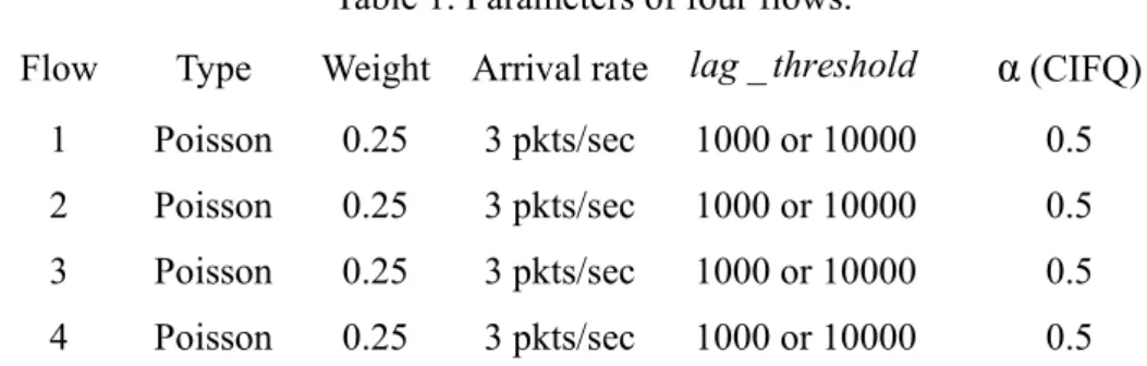
Table 1. Parameters of four flows...38

Table 2. The various channel state distributions...46

Table 3. Parameters of four flows with different service weights...50

(7)

List of Figures

Part I

Fig. 1. The proportional differentiation model...11

Fig. 2. The proportional differentiation model in a wireless network...13

Fig. 3. The LWTP Algorithm...17

Fig. 4. The effect of packet arrival rates...21

Fig. 5. The effect of different mean channel capacity (with the fixed variance 1016) ...23

Fig. 6. The effect of different variances of channel capacity (with the fixed mean 1323 bytes/sec) ...24

Fig. 7. The effect of the number of mobile hosts...26

Fig. 8. Average waiting times of LWETP and WWTP with different channel thresholds...28

Part II

Fig. 1. The algorithm of EFQ...36

Fig. 2. Throughput and average delay of four flows in EFQ_1000...39

Fig. 3. Throughput and average delay of four flows in CIFQ_A...40

Fig. 4. The fairness under various short timescales... ...41

Fig. 5. The average delay under various short timescales...42

Fig. 6. Fairness, average delay, and mean service capacity under various packet

(8)

arrival rates...44

Fig. 7. Fairness and average delay under different channel transition rate...45

Fig. 8. Fairness and average delay under various channel state distribution... 47

Fig. 9. Fairness and average delay under various access criteria in CIFQ...49

Fig. 10. Ratios of four flows receiving service in EFQ_1000 and CIFQ_B...51

Fig. 11. Throughputs of four flows under different weights in EFQ_1000 and CIFQ_B...52

(9)

Part I: Proportional Delay Differentiation

1 Introduction

With the rapid development of many new applications in the Internet, best-effort service is no longer sufficient to satisfy their QoS requirements. For example, the individual may tolerate a longer waiting time or a larger packet loss because he/she only pays low costs, while the enterprise is probably willing to pay more money to receive better services for their network traffic. Consequently, providing multiple levels of QoS in the Internet becomes a very important issue.

In 1990 the Internet Engineering Task Force (IETF) formed the Integrated Services working group. The integrated services (IntServ) architecture was then proposed to fulfill applications’ and users’ requests with a certain performance guarantee using the resource reservation protocol (RSVP) and an admission control mechanism [1]. An application requesting QoS requirement must characterize its flow specification. The PATH signal goes hop by hop from a sender to a receiver and then the RESV signal returns backward along this path to reserve network resources. The admission control is responsible for monitoring the resource usage and deciding whether to grant or deny a request. The IntServ architecture uses per-flow resource reservation, resulting in an un-scalable problem.

Due to those difficulties faced by the IntServ architecture, by 1997 the IETF formed a new group, the Differentiated Services working group, to develop a more scalable architecture, the Differentiated Services (DiffServ) architecture, for providing multiple levels of users’

requirements [2]. Under the DiffServ framework, the traffic requesting the same QoS requirement will be aggregated into a corresponding service class. Thus the granularity of service level of the DiffServ is reduced from an individual flow to a class, an aggregation of flows, so that the un-scalability problem can be alleviated. Many differences exist between the IntServ and the DiffServ architectures, and their detailed comparison can be found in [3].

Currently, the DiffServ has evolved in two directions: absolute differentiated services and relative differentiated services. The absolute differentiated services grant users certain performance guarantee, while the relative differentiated services classify users’ traffic into

(10)

different priority classes and provide higher priority classes with better (or at least no worse) services than lower priority ones. In terms of further taxonomy of service differentiation, the absolute differentiated services have two branches: premium services [4] and assured services [5], and the relative differentiated services have five models: strict prioritization, price differentiation, capacity differentiation, additive differentiation, and proportional differentiation [6]. Our report focuses on the proportional differentiation model for it can provide controllable and predictable service differentiation [6]. Specifically, the proportional differentiation model provides a network manager with a means to manipulate the quality spacing between service classes according to the given pricing or policy criteria, and it also ensures that the differentiation between classes is consistent in any measured timescale.

In the proportional differentiation model, the performance metrics is often regarded as packet queueing delay or packet loss rate. C. Dovrolis et al. proposed the Waiting-Time Priority (WTP) scheduler to approximate the desired proportional delay differentiation under heavy traffic load [6]. Later they also proposed two droppers, PLR(∞) and PLR(M), to approximate the proportional loss differentiation model [7]. S. Bodamer proposed the weighted earliest due date (WEDD) algorithm to provide tunable delay differentiation for applications with a mechanism that has not only different delay bounds but also different deadline violation probabilities [8]. A. Striegel et al. proposed the Class Distance Based Priority (C-DBP) scheduler to provide proportional differentiation and claimed that this scheduler offers the freedom of QoS selections in which the delay and loss can be chosen independently [9].

These studies do have remarkable contributions, however, only in the wired environment.

With the technology rapidly advances in wireless communication and the popularity of lightweight portable computing devices, a wireless network environment has been more and more pervasive. Therefore, providing proportional delay differentiation in a wireless environment is urgent just as it was in the wired network. However, the previous approaches designed in a wired network are not applicable in a wireless environment due to some specific characteristics of a wireless link, namely, 1) high error rate and burst errors; 2) location-dependent and time-varying capacity; 3) scarce bandwidth [10]. These characteristics, if without being specially and carefully treated in designing a scheduler, often cause the HOL

(11)

blocking problem and low channel utilization.

This report proposes a novel scheduler, which can provide the proportional delay differentiation in a wireless network with a multi-state channel. Our proposed LWTP scheduler, modified from the WTP scheduler, tries to transmit packets to a mobile host which has a high-capacity channel and maintain the proportional delay differentiation simultaneously. Thus the LWTP scheduler can obtain the following characteristics: 1) to provide proportional delay differentiation; 2) to offer lower queueing delay; 3) to conquer head-of-line (HOL) blocking problem.

The structure of this report is as follows. Some related works concerning the proportional delay differentiation and the packet scheduling over wireless network are presented in Section 2. Section 3 proposes our LWTP scheduler. Section 4 presents the simulation results and discusses their implications. Finally, conclusions are given in Section 5.

2 Background

2.1 Proportional Differentiation Model

The proportional differentiation model was proposed by C. Dovrolis et al. to provide relative quality spacing between classes [6]. This model has two objectives: to be controllable and to be predictable. To be controllable means that the network manager has a means, in the authors’

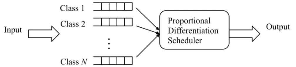
words, ‘tuning knobs’, to control and adjust the quality spacing for different classes, based on his/her criteria. To be predictable means that whatever the traffic load of classes is, traffic belonging to higher priority classes should always receive better performance (at least no worse) levels than that belonging to lower ones. Fig. 1 depicts the proportional differentiation model.

(12)

Input

…

Class 1

Class 2

Class N

Proportional Differentiation Scheduler

Output

Fig. 1. The proportional differentiation model.

Considering N classes of services, each class has a dedicated queue. The proportional differentiation scheduler is responsible for scheduling packets from the N classes and providing differentiated services. Let q denote the performance measure of class i. Assume _i class j has higher priority than class i, where i < j. The proportional differentiation model is described by the following proportionality constraint for any pair of classes:

j i j i

c c q

q = (1 ≤ i, j ≤ N) (1)

where 0 < c₁ < c₂ < … < c_N , and c_i is the quality differentiation parameter (QDP) of class i. A network manager could manipulate the service quality spacing between classes by adjusting the QDPs. The performance metrics is often regarded as packet queueing delay or packet loss rate. Let d_i denote the average queueing delay of class-i packets. Assume class j is expected to have shorter average queueing delay than class i does, where i < j. The proportional delay differentiation model has the following constraint for any pair of classes:

j i j i

d d

δ

= δ (1 ≤ i, j ≤ N) (2)

where δ1 > δ2 > … > δN > 0, and δi is the delay differentiation parameter (DDP) of class i.

Correspondingly, the proportional loss differentiation model uses packet loss rate as performance metrics. However, herein we concentrate on how to provide proportional delay differentiation in a wireless network.

(13)

2.2 WTP

The WTP scheduler was originally from Kleinrock’s Time-Dependent-Priorities algorithm, a non-preemptive packet scheduling algorithm that provides a set of control variables to manipulate the instantaneous priority of any packet [11]. In WTP, the priority of a packet increases in proportion to its waiting time. Let P_i^k(t) denote the priority of the k-th packet of the class i at time t, and W_i^k(t) be its waiting time. Then, the priority is set as

i k i k

i

t t W

P δ

) ) (

( = (1 ≤ i ≤ N) (3)

where δ1 > δ2 > … > δN > 0, and δi is the delay differentiation parameter (DDP) to control the priority increasing rate for certain class.

Among each class, the HOL (i.e., k=1) packet has the longest waiting time than any packet else behind it, so only the HOL packet of each class has to be considered for scheduling. Thus Eq. (3) is re-expressed as follows,

i i i

t H t W

P δ

)) ( ) (

( = (1 ≤ i ≤ N) (4)

where W(Hi(t)) is the waiting time of the HOL packet of class i at time t.

WTP is examined to successfully approach the targeted delay proportion under heavy load, but does not achieve it under light load. Thus many works have been done to solve the unachievement of delay proportion under the light-load condition. C. Dovrolis et al. later proposed a hybrid proportional delay (HPD) scheduler, which combines WTP and PAD, to provide proportional delay differentiation regardless of class load distribution [12]. H. Saito et al. proposed a local optimal proportional delay packet scheduler, which reaches an optimal decision when no further packets are arriving and induces more accurate approximations of delay ratio than WTP does [13]. Matthew K. H. Leung et al. proposed an adaptive control algorithm by adjusting some control parameters in response to the variable system load [14].

2.3 Problems of Scheduling over Wireless Network

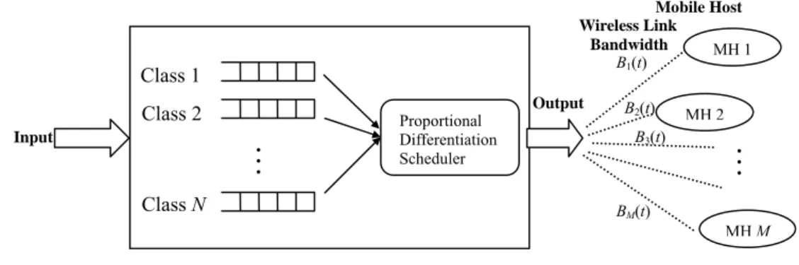
Fig. 2 illustrates the proportional differentiation model in a wireless network. In this model, all

(14)

…

Class 1

Class 2

Class N

Proportional Differentiation Scheduler

MH 1

MH 2

MH M

…

Wireless Link Bandwidth

B1(t)

B2(t) B3(t)

BM(t) Input

Output

Mobile Host

mobile hosts share one link. Because each host could be located at different locations, different capacities appear when this scheduler transmits data to different mobile hosts via the same wireless link. Also as the mobile host moves, the capacity to this host varies. Thus a wireless link has a location-dependent and time-varying capacity. For clear description, a logical channel (for simplicity, we call "channel" in this report) can be regarded as a wireless link to a mobile host. Note that more than two channels are concurrently used is impossible because only one wireless link actually exists. Let B_j(t) denote the channel capacity when the scheduler transmits packets to a mobile host j at time t.

In a TDMA network, a wireless channel has either full capacity when it is error-free or zero capacity when it is error-prone, that is, Bj(t) = L or Bj(t) = 0, where L is full capacity. Thus an individual channel can be modeled by employing a two-state Markov chain, which including error-free and error-prone states. When any channel has zero capacity (B_j(t) = 0), a HOL blocking problem may happen in this channel, especially when many input flows are aggregated into a small number of classes. HOL blocking is that more than two packets are in the same queue and the HOL packet cannot be served because of its bad destined channel, then all packets behind this HOL packet in the same queue can not be served even their destined channels are good. So, subtle considerations need to be put into a new wireless approach, just like WWTP in later subsection.

Fig. 2. The proportional differentiation model in a wireless network.

However, a channel in a CDMA network contains multiple states other than just good or

(15)

bad state, and each state has its own capacity (i.e., B_j =α_iL, where 0≤α_i≤1). Thus a HOL blocking problem still happens in a CDMA network when a channel has zero capacity (α_i = 0).

Besides, a serious problem of low throughput should be considered. When a channel capacity is scarce, i.e. αi is close yet not equal to zero, transmitting packets on this channel would take a long time, which results in a low throughput and a long packet queuing delay. Thus, a scheduler should note the channel condition to obtain the high throughput in this CDMA environment.

2.4 WWTP

Due to the current schedulers designed for wired communications are inapplicable for wireless networks, M. R. Jeong et al. modified the WTP scheduler and proposed a Wireless WTP (WWTP) scheduler to provide relative delay differentiation [15] in the wireless network in which wireless links have only two states (i.e. error-free or error-prone). They assume that the scheduler has full information of each link so it can avoid transmitting packets on an error-prone channel. WWTP serves a packet that has the highest priority and error-free destined channel at each scheduling time. The steps are taken as the followings.

1) Choose HOL packets of each non-empty queue initially.

2) Calculates the priority value,

i i i

t H t W

P δ

)) ( ) (

( = , for each HOL packet.

3) Compares the calculated priority values of all chosen packets. Selects the packet from the class with the largest priority value, and then checks the destined channel state of the selected packet.

4) If the destined channel state is error-free, transmits the selected packet. Otherwise, excludes the selected packet from scheduling and chooses the subsequent packet of the same class instead. Re-calculates the priority value of this new packet. Goes to step 3.

WWTP can avoid the HOL blocking problem by excluding those packets suffering channel errors from transmission. Once those packets’ destined channels recover from bad to good, those packets would get compensated, since their waiting times accumulate and the priority

(16)

values increase during the channel error durations.

3 The LWTP Scheduler

Assume the scheduler can fully identify the channel status of every mobile host. Each channel has multiple states, not just good or bad state. Our proposed LWTP scheduler has the following goals in a multi-state wireless network: 1) to provide proportional delay differentiation, 2) to offer low queueing delay, and 3) to conquer the HOL blocking problem.

LWTP does scheduling in two phases: avoiding HOL blocking in phase I and then increasing throughput and keeping the proportional delay differentiation in phase II. This scheduler prefers transmitting packets on channels with better capacity to reduce the overall waiting time and increase throughput.

In phase I, LWTP finds out exact one candidate, rather than a HOL packet, in each non-empty queue. A packet will be selected as a candidate only when its destined wireless channel has any capacity except zero. Initially, candidate packets are the HOL packets from all non-empty queues. If any candidate is blocked, then this packet is substituted with the subsequent one of the same queue until a packet with non-zero destined channel capacity is encountered or the end of the queue is reached. Let Cj(t) be the candidate of class i at time t. It may be NULL if all packets in the queue are blocked or in an empty queue.

In phase II, LWTP employs a pseudo-service technique, which virtually transmits the candidate packet in turn and evaluates the virtual new waiting times of all candidate packets after that has been transmitted. Let W(C_j(t)), PS(C_j(t)), and B(C_j(t)) denote the waiting time, packet size, and destined channel capacity of the candidate Cj(t) at time t, respectively.

When the pseudo-served packet belongs to class i, LWTP calculates the virtual normalized waiting time of class j, V_jⁱ(t), and obtain the maximum proportion, MPi(t), as,

⎪⎩

⎪⎨

⎧

≠

= + =

= , if .

)) ( (

; if , 0 where

)) , ( ) (

( j i

t C B

t C PS

i j X X

t C t W V

i i i

j i i j

j δ (5)

)}.

( { max )

(t 1 V t

MP _jⁱ

N

i = ≤i≤ (6)

(17)

X_i is the extra waiting time caused by transmitting the candidate packet of class i. For each class i, its corresponding MP_i(t) is calculated. Then, the minimum value of all MP_i(t), and the corresponding index are determined by,

)};

( { min )

(t 1 MP t

MMP _i

i≤N

= ≤ (7)

)}.

( { argmin )

(

1

t MP t

S _i

i≤N

≤

= (8)

The LWTP scheduler chooses the candidate packet of class S(t) and actually transmits it.

When more than one MP_i(t) equals MMP(t), LWTP randomly selects one of them.

The fundamental concept of LWTP is to preview the influence brought by a packet selected for transmission. By adopting the pseudo-service of candidate packets, LWTP compares and reduces the difference between the normalized waiting times of all candidates, and then transmits the packets which yield the most accurate proportion. When pseudo-servicing a packet of class i, the obtained maximum proportion MP_i(t) implies the most over-proportional value. A larger MP_i(t) corresponds to a poorer proportion. Thus LWTP selects the packet with the minimum MP_i(t), that is, the most correct proportion. The detail LWTP algorithm is shown in Fig. 3.

Consider an example of three classes (N = 3) and let the current queuing delays of three candidate packets be W(C₁(t))=0.5, W(C₂(t))=0.8, and W(C₃(t))=1.0 time units. Their packet size are PS(C₁(t))=PS(C₂(t))=PS(C₃(t))=441 bytes, and current destined channel capacity are B(C₁(t))=1323, ))B(C₂(t =2646, and B(C₃(t))=661.5 bytes/sec. The DDPs for the three classes are δ₁=1, δ₂=2, and δ₃=4. For WWTP, the priorities of the candidate packets at time t are P₁(t)=0.6, )P₂(t =0.4, and P₃(t)=0.25; consequently, the WWTP algorithm delivers the candidate packet of class 1. By employing Eqs. (5) and (6), given in Table 1, the LWTP algorithm calculates MP1(t)=0.733, MP2(t)=0.667, and MP3(t)=0.833, represented as underlined, and gives MMP(t)=0.667 and S(t)=2, marked by an oval. Thus LWTP selects the candidate packet of class 2 to transmit. The selections of the WWTP scheduler (class 1) and the LWTP scheduler (class 2) are clearly different.

(18)

Table 1. An example for the LWTP algorithm.

j=1 j=2 j=3 Pseudo-service of class-1 packet (i=1) 0.5 0.733 0.417 Pseudo-service of class-2 packet (i=2) 0.4 0.292 Pseudo-service of class-3 packet (i=3) 0.833 0.567 0.25

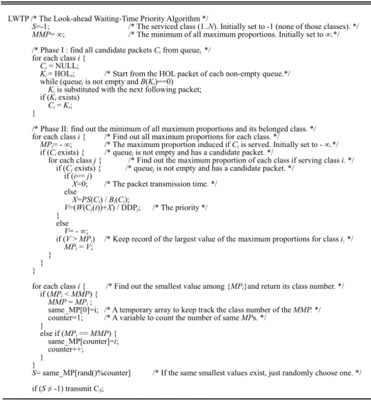
Fig. 3. The LWTP Algorithm.

LWTP /* The Look-ahead Waiting-Time Priority Algorithm */

S=-1; /* The serviced class (1..N). Initially set to -1 (none of those classes). */

MMP= ∞; /* The minimum of all maximum proportions. Initially set to ∞.*/

/* Phase I : find all candidate packets Ci from queuei. */

for each class i { Ci = NULL;

Ki = HOLi; /* Start from the HOL packet of each non-empty queue.*/

while (queuei is not empty and B(Ki)==0) Ki is substituted with the next following packet;

if (Ki exists) Ci = Ki; }

/* Phase II: find out the minimum of all maximum proportions and its belonged class. */

for each class i { /* Find out all maximum proportions for each class. */

MPi= - ∞; /* The maximum proportion induced if Ci is served. Initially set to - ∞.*/

if (Ci exists) { /* queuei is not empty and has a candidate packet. */

for each class j { /* Find out the maximum proportion of each class if serving class i. */

if (Cj exists) { /* queuej is not empty and has a candidate packet. */

if (i== j)

X=0; /* The packet transmission time. */

else

X=PS(Ci) / Bi(Ci);

V=(W(Cj(t))+X) / DDPj; /* The priority */

} else V= - ∞;

if (V > MPi) /* Keep record of the largest value of the maximum proportions for class i. */

MPi = V;

}

for each class i { /* Find out the smallest value among {MPi}and return its class number. */

if (MPi < MMP) { MMP = MPi ;

same_MP[0]=i; /* A temporary array to keep track the class number of the MMP. */

counter=1; /* A variable to count the number of same MPs. */

}

else if (MPi == MMP) { same_MP[counter]=i;

counter++;

} }

S= same_MP[rand()%counter] /* If the same smallest values exist, just randomly choose one. */

if (S ≠ -1) transmit CS;

0.667

(19)

In particular, the LWTP scheduler exhibits the following characteristics.

z No HOL blocking occurs. Through the process of looking for candidate packets, the HOL blocking problem is eliminated. If the current candidate is blocked, then this packet is substituted with the subsequent one of the same queue until a packet with non-zero destined channel capacity is encountered or the end of the queue is reached. Therefore, the candidate will not encounter the bad channel, and thus the HOL blocking problem never occurs.

z Delay proportion is maintained. For a packet whose destined channel is in error burst, the duration is accumulated into this packet’s waiting time. After the channel’s recovery, the packet would get a very high priority to get its bandwidth compensation. Also the LWTP scheduler selects the packet which generates the minimum MP_i(t) to keep the average waiting times for all classes as proportional to the given DDPs. Thus, LWTP can meet the target ratio as close as possible.

z Packet destined to the channel with higher capacity is preferred. A packet with poor capacity of destined wireless channel often results in longer transmission time, which leads to a larger maximum proportion. Thus, it is less likely to be selected and give the opportunity to a packet with better destined channel capacity. A short packet transmission time only causes few differences between the pseudo waiting time and the current waiting time, so its MP is typically small and more likely to be selected as MMP. Consequently, the LWTP scheduler prefers packets with shorter transmission time, that is, it prefers the packet destined to the high-capacity channel.

z Packet of the class with higher priority is preferred. WWTP and LWTP all prefer the packets of higher priority classes because of its lower DDPs. However, LWTP more strongly prefers the packets of higher-priority class than does WWTP. For LWTP, when the pseudo-served packet belongs to higher priority class, its transmission time is divided by a larger DDP, giving a smaller MP. Thus, the packet of higher priority class is more likely to be selected. For example, suppose there are three classes ordered with DDPs as 4, 2, and 1 respectively. When the current waiting times of all candidate packets are in the ratio, 4:2:1, WWTP randomly selects a packet while LWTP selects the higher-priority-class packet when all candidate packets are of equal transmission time.

(20)

z LWTP behaves differently from WWTP except when waiting time is very large or traffic is light-loaded. When the waiting time is quite large relative to the transmission time, the effect of considering the latter will be minor. Because the waiting time increases with the arrival rate, LWTP might behave like WWTP does when the arrival rate is high enough to cause many packets backlogged. On the other hand, when packet arrival rate is so low that the offered traffic load is far fewer from the service capacity, LWTP has no many other choices to make since there are only few packets existing in all queues. In such a case, LWTP also behaves like WWTP.

4 Simulation Study

The simulation studies evaluate the WWTP and LWTP packet schedulers in the context of the proportional delay differentiation model over a wireless link, which has a time-varying, location-dependent, and multi-state capacity. The simulations are conducted to investigate the effects of packet arrival rate, mean channel capacity, variance of channel capacity, and number of mobile hosts on the delay ratio and delay improvement, whose definitions are described later.

The model we simulate is depicted as in Figure 2. There are three service classes (N=3).

The DDPs are set as δ1=1, δ2=2, and δ3=4. Packet arrival follows a Poisson process and its mean arrival rate is λ=0.9 packets/sec. The packet size is fixed at 441 bytes for all classes. The buffer size for each class is infinite, i.e., no packet loss, and the full wireless channel capacity is 2646 bytes/sec. The wireless channel, which is modeled by a multi-state Markov chain, has five states with the capacity varying among 100%, 75%, 50%, 25%, and 0% of the full capacity. The Markov chain transition matrix of channel capacity is set as

⎥ ⎥

⎦

⎤

⎢ ⎢

⎣

⎡

a p

a p a p a p a

p a a

p a p a p a

p a p a a

p a p a

p a p a p a a

p a

p a p a p a p a a

2 5 3 5

4 5 5

4 2 4

3 4 4

32 3

2 3 3

23 22

2 2

14 13

12 1

) - (1 ) - (1 ) - (1 ) - (1

) - (1 )

- (1 ) - (1 ) - (1

) - (1 ) - (1 )

- (1 ) - (1

) - (1 ) - (1 ) - (1 )

- (1

) - (1 ) - (1 ) - (1 ) - (1

% 0

% 25

% 50

% 75

% 100

. 100% 75% 50% 25% 0%

(21)

The default value of a is 0.8, and the values of p₁, p₂, p₃, p₄, and p₅ can be calculated by letting the sum of each row equal to 1. In each simulation, at least 500,000 packets for each class are generated for the sake of stability.

The average queueing delay of class i, d , is obtained by averaging the measured delays i

of all serviced class-i packets. The performance metrics used in this report for comparing WWTP with LWTP are delay ratio and delay improvement. The delay ratio of class i over class j is defined as d /i d j and the delay improvement of class i is defined as

W i L i W

i d D

d )

( − , where d^Wi and di^L are the average queueing delays of class i, made by WWTP and LWTP, respectively.

4.1 Packet Arrival Rate

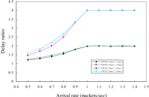
To observe the influence of different packet arrival rates on achieved delay ratios and delay improvement, the arrival rate (λ) is varied from 0.5 to 1.4 packets/sec. The target delay ratios are 4 (δ3/δ1=4/1) for class 3 over class 1, and 2 (δ2/δ1=2/1) for class 2 over class 1. Fig. 4(a) shows that the delay ratios achieved by both WWTP and LWTP reach the target ratios when the arrival rate exceeds 1.0 packets/sec, which is heavy traffic load. At high packet arrival rate, the packet waiting time greatly exceeds the packet transmission time, and thus LWTP and WWTP make the decision quite similar to each other. Nevertheless, when traffic load is moderate, neither WWTP nor LWTP approaches the desired delay proportion. However, LWTP has delay ratios higher than WWTP has, since the former prefers the packets of higher-priority class (herein, class-1 packets) than does the latter. At low packet arrival rate, LWTP has few choices different from WWTP, thus both have similar behaviors.

Fig. 4(b) reveals that the queueing delay improved by LWTP increases as packet arrival rate increases, but to an extent, the improvement starts to decrease. The reason is the same as discussed above. Another fact to notice is that under moderate traffic arrival rate, the delay improvements of each class by LWTP are class 1 > class 2 > class 3, since LWTP prefers packets of higher-priority class.

(22)

0 0.5 1 1.5 2 2.5 3 3.5 4 4.5

0.4 0.5 0.6 0.7 0.8 0.9 1 1.1 1.2 1.3 1.4 1.5

Arrival rate (packets/sec)

Delay ratios

WWTP: Class 2 / Class 1 WWTP: Class 3 / Class 1 LWTP: Class 2 / Class 1 LWTP: Class 3 / Class 1

(a) Delay ratios

-505 1015 20 25 30 35 40 4550 55 60 65 70 75 8085 90 95 100

0.4 0.5 0.6 0.7 0.8 0.9 1 1.1 1.2 1.3 1.4 1.5

Arrival rate (packets/sec)

Dealy improvement (%

Class 1 Class 2 Class 3

(b) Delay improvement

Fig. 4. The effect of packet arrival rates.

(23)

4.2 Mean Channel Capacity

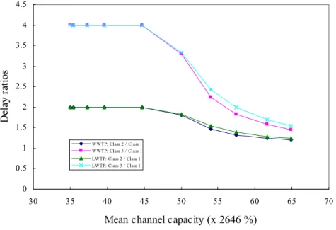
The channel capacity is absolutely associated with the channel state. The mean channel capacity is varied, with the variance fixed at 1016, to observe the behaviors of WWTP and LWTP for the achieved delay ratios and delay improvement. Fig. 5(a) reveals that when channel capacity is small, both WWTP and LWTP achieve the target ratios. But as channel capacity increases, both schedulers’ ratios slide down. The reason is that we fix the arrival rate for each class at 0.9 packets/sec, so the traffic becomes heavy-loaded when channel capacity is small, while moderate-loaded when channel capacity is large. Thus the consequence comes in the same way as the previous discussion of packet arrival rate. Still, LWTP has closer ratios to the target than WWTP. In Fig. 5(b), the queueing delay improved by LWTP increases as mean channel capacity increases, but to an extent, the improvement starts to decrease.

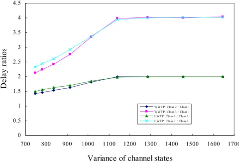
4.3 Variance of Channel Capacity

The channel capacity is varied, with the mean fixed at 1323 bytes/sec, to see the effect of capacity variance on the achieved delay ratios and delay improvement. Fig. 6(a) shows that when the variance is large, both WWTP and LWTP approximate the target ratios, but when the variance is small, both schedulers cannot maintain their desired ratios. Smaller variance represents more number of states near the mean, while larger variance represents more number of states far away from the mean. Fig. 6(b) reveals that the queueing delay improved by LWTP increases as the variance of channel state increases, but to an extent, the improvement starts to decrease. When most of the channels are at the mean state, LWTP has few choices different from WWTP, so the improved delay ratio is small.

(24)

0 0.5 1 1.5 2 2.5 3 3.5 4 4.5

30 35 40 45 50 55 60 65 70

Mean channel capacity (x 2646 %)

Delay ratios

(a) Delay ratios

-5 0 5 10 15 20 25 30 35 40 45 50 55 60 65 70 75 80 85 90 95 100

30 35 40 45 50 55 60 65 70

Mean channel capacity (x 2646 %)

Delay improvement (%)

Fig. 5. The effect of different mean channel capacity (with the fixed variance 1016).

(25)

0 0.5 1 1.5 2 2.5 3 3.5 4 4.5

700 800 900 1000 1100 1200 1300 1400 1500 1600 1700

Variance of channel states

Delay ratios

(a) Delay ratios

-505 1015 2025 3035 4045 50 5560 6570 75 8085 9095 100105

700 800 900 1000 1100 1200 1300 1400 1500 1600 1700

Variance of channel states

Delay Improvement (%)

Fig. 6. The effect of different variances of channel capacity (with the fixed mean 1323 bytes/sec).

(26)

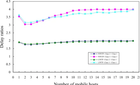
4.4 Number of Mobile Hosts

The number of mobile hosts is varied from 1 to 20 to investigate the influence on achieved delay ratios and delay improvement. Packets of each class is distributed and destined evenly to each mobile host. Fig. 7(a) shows the number of mobile hosts does not affect the delay ratios quite much as the number exceeds 10. Fig. 7(b) reveals that the queueing delay improved by LWTP increases as the number of mobile hosts increases, but after the number exceeds 10, the improvement becomes stable and stays near 90%. When there are only a few mobile hosts, LWTP has rare channel to be chosen so that the delay improvement is not high. As the number of mobile hosts increases, since LWTP prefers packets destined to higher-capacity channel while WWTP only cares of packet’s waiting time, the delay improvement made by LWTP increases.

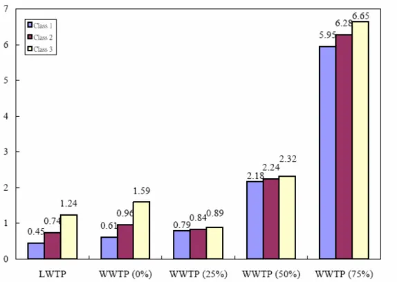
4.5 Comparison of LWTP to WWTP with a Threshold

In the earlier simulations, WWTP could transmit a packet when its destination channel was not in a purely bad state. In an environment with a multi-state link, the other approach is taken:

WWTP does not transmit any packet unless its destination channel is wholly good. This approach causes the wireless link not to be well utilized when all channels do not remain totally good (100% capacity). These two extreme approaches for applying WWTP to a multi-state link are direct, but not good enough. Therefore, we modify the original WWTP to facilitate this wireless environment and observe whether the proposed LWTP can outperform it.

WWTP is modified by adopting a channel threshold to regulate the usage of any channel.

Unless the channel capacity exceeds this threshold, WWTP temporarily bypasses all of the packets destined to this channel until the condition is satisfied. Accordingly, a channel is distinguished as PASS or BLOCK, depending on whether its capacity exceeds this threshold.

Step 3 of the WWTP algorithm in Sec. 2.4 is modified as follows.

(27)

0 0.5 1 1.5 2 2.5 3 3.5 4 4.5

0 1 2 3 4 5 6 7 8 9 10 11 12 13 14 15 16 17 18 19 20 21

Number of mobile hosts

Delay ratios

(a) Delay ratios

-505 1015 2025 3035 4045 5055 6065 7075 8085 9095 100105

0 1 2 3 4 5 6 7 8 9 10 11 12 13 14 15 16 17 18 19 20 21

Number of mobile hosts

Delay improvement (%)

Fig. 7. The effect of the number of mobile hosts.

(28)

“Check the state of the destination channel state of the chosen packet. If this state is better than the channel threshold, transmit the chosen packet. Otherwise, exclude the chosen packet from scheduling and choose the subsequent packet in the same queue. Recalculate the priority of this new packet using Eq. (3), and then go to Step 2.”

The scenario considered herein involves four possible channel thresholds - 0%, 25%, 50% and 75% of the full link capacity. The algorithm that uses thresholds 0% and 75%

corresponds to WWTP's avoiding the selection of totally bad channels and insistence on selecting totally good channels, respectively.

Figure 8 reveals the average waiting times for WWTP under given various channel thresholds. For WWTP, adopting a threshold channel usage may reduce the overall waiting time (such as when the channel threshold is increased from 0% to 25%); however, an excessively strict channel threshold increases waiting time (such as when the channel threshold is increased from 25% through 50% to 75%). The reason is because excluding poor channels may shorten the overall waiting time since transmitting packets on these channels is time-consuming, yet making the constraint stricter may increase the overall waiting time since the channels stay in PASS state only occasionally, and thus no packet can be transmitted when all channels stay in the BLOCK state.

As the channel threshold is made stricter, the opportunities for many channels to be BLOCK increase. If a specific channel must be selected to achieve the target delay proportion while it is unfortunately in the BLOCK state, then the required delay proportion will be hard to maintain. A stricter threshold corresponds to remaining in the BLOCK state for longer, resulting in a worse delay proportion. However, remaining in the BLOCK state for longer also increases waiting time, indirectly making the delay ratio closer to the target proportion. By combining these two effects, the achieved delay ratio made by WWTP initially declines and then increases as the channel threshold moves from 0% to 75%.

The WWTP with a threshold has three weaknesses. The first is that under particular channel thresholds, the average waiting time decreases, whereas the target delay proportion can not be simultaneously maintained, such as when threshold=25%. The second is that determining an appropriate channel threshold that yields both an accurate delay ratio and a low queueing delay is difficult in a realistic wireless network. The third is that the channel

(29)

threshold is static and cannot adapt to ever-changing wireless channels.

Figure 8 also reveals that LWTP has a shorter delay than WWTP whose threshold is set to 0%, 50% or 75%. LWTP yields a more accurate delay ratio than WWTP in all cases. The correct delay proportion should be more important than the low queueing delay in the proportional delay differentiation model, so WWTP uses threshold=0% as the most feasible threshold, and thus Subsection 4.2 to 4.6 compare this WWTP with LWTP. In contrast to WWTP with a threshold, LWTP considers dynamic channel states and chooses the most qualified channel to provide proportional delay differentiation with competent performance (low delay). Also, the threshold is not needed so LWTP does not suffer from the three drawbacks of WWTP.

Fig. 8. Average waiting times of LWETP and WWTP with different channel thresholds.

5 Conclusions

The characteristics of time-varying channel capacity and location-dependent error exhibited in