生活史特徵與漁撈壓力對魚類族群空間分布的變異度-平均值關係之影響

國立臺灣大學理學院海洋研究所 碩士論文

Institute of Oceanography College of Science

National Taiwan University Master Thesis

生活史特徵與漁撈壓力對魚類族群空間分布的變異度- 平均值關係之影響

Influences of life history traits and fishing on the spatial variance-mean relationship of fishes

郭庭君 Ting-Chun Kuo

指導教授：謝志豪 博士 Advisor: Chih-hao Hsieh, Ph.D.

中華民國 101 年 6 月

June, 2012

致謝

終於要畢業了，但在這刻心中仍沒有塵埃落定的感覺，也許是因為論文還要 修訂，也可能是未知的未來橫在眼前，所以心慌多於欣喜。碩士短短的兩年倏乎即 逝，日日周旋於大小死線的追趕、不如預期的研究成果與生活中的零零總總，回頭 來看，辛酸疲累的感覺已經都淡了，只記得其中每個甜美的時刻（也許就是因為這 種健忘性格，才能一直在學術之路繼續走下去？），而這段路程每步小小的前進，

都深受許多人的幫忙。

首先感謝我的指導老師謝志豪老師，謝謝您一路上自由卻不放任的指導，也總 是在我需要幫助的時候，隨時放下手邊的工作跟我討論，而且每一次的討論都讓我 受益良多。老師的訓練，不僅讓我們扎實地完成一份科學研究中各階段該做的事，

也為我們定下了一道標準：如何讀文獻、如何品味別人的研究成果、如何發想題目、

設計方法、整理自己的研究結果、撰寫報告等，雖然我並不是每項都能做得很好，

但是希望離開了老師以後，還是能拿這套標準要求自己，不要鬆懈。老師，在這兩 年中我一定很常讓您擔心，雖然您一開始就警告過我要衡量自己的時間，不要做太 多個 project，但我還是兩個都放不下，以致於最後都很倉促，其實自己也很挫敗。

我會謹記這個教訓的，謝謝您給我的包容和幫助。

再來，感謝撰寫論文中曾經幫助我的老師們：三木健老師， 您的課為我開啟了 理論生態的一扇大門，到後來在建模的過程中，也給了我很多幫助。王慧瑜老師，

在這一年中給我的許多不論是論文還是申請學校方面建議，都幫助很大，每次和老 師聊天，心中也會平靜許多，有種神奇的力量！另外還有我的口委許建宗老師與沈 聖峰老師，在口試時也給了我許多有建設性的建議，能有人耐心了解自己的研究，

真的是一件令人感激涕零的事。當然還有從高中時期就一直給予我指導和建議的于 宏燦老師，若沒有在您實驗室的經歷，不會開啟我走向研究之路的大門。我大學時 期的導師黃玲瓏老師，老師對待導生們就像對待自己的孩子一樣，三不五十就會關

心我們 。另外還有修課過程中影響過我的郭鴻基、陳俊良、黃火煉、陳金次老師等，

雖然您們可能不記得我，但今天我決定選擇這個領域，都是深受您們的課程的啟發。

當然也非常感謝實驗室的夥伴，怡君、貓和奧斯卡，在兩年中一起互相鼓勵、

開玩笑、吃飯、玩耍、出國冒險，沒有你們在身邊，我的碩士生活一定會失色非常 多。422 的大家，小平、小點、欣穎、菜蟲、俊偉、君屹、Carmen、Take、Crystal、

珮琦、瑋婷、冠婷、拉狗、煒忠、梵絃、柏如、小柏、阿伯....因為有你們，我每 天去實驗室都很開心，也謝謝你們在我快樂的時候為我高興、失意的時候鼓勵我、

給我建議，想到離開你們，是我最捨不得的事。也謝謝生科系 B95、94、96 的夥伴，

生科系四年是我一輩子難忘的回憶；謝謝我的高中同學們，讓我永遠記得人生中的 單純美好。

謝謝 H，你讓我體會了人生許多事，願你之後順利。謝謝凱淯，總是支持、幫助 我做我想做的事，也教會我用許多有趣的方法看世界。最後最後，當然最要感謝的 就是我的家人，你們總是無條件的支持我，雖然你們總是搞不懂我在做什麼，卻還 是願意相信我，讓我盡情發揮，也是我最堅強的後盾。我愛你們。

摘要

前人的研究指出，族群在空間中的豐度平均值(M)與變異度(V)呈現一冪次關

係（泰勒冪次定律），意即V=aM^b。許多因子可能影響指數b，如聚集程度、生長速率

與繁殖率等；然而，係數 a 所代表的意義卻尚無定論。本篇研究中，我們估算了一

九五一年至二〇 〇七年，南加州洋流生態系中二十九種海洋魚類族群豐度的空間平

均值與變異度關係。我們並檢驗各物種的泰勒指數（b）是否會受到該物種的生活史

特性影響。另外，在考量生活史特性的差異後，我們也藉由一般線性回歸（General Linear Model）比較商業目標魚種與非目標魚種的泰勒指數，檢驗漁業對魚類空間 分布的影響。結果顯示，排除平均豐度的影響後，所有的生活史特徵都會與泰勒指 數成顯著線性相關。以非目標魚種來說，具有 r 生殖策略相關特徵的物種具有較高 的泰勒指數; 然而，於漁業目標魚種中此現象卻不顯著。這可能是由於漁業壓力改 變了目標魚種的族群平均生活史特徵（如最大體長），使得目標魚種有較高的泰勒指 數，亦即分布變得較為密集。我們也建立了一個體基準模型（individual-based model），探討泰勒冪次定律的形成過程，以及改變族群年齡結構後，是否會改變泰 勒指數。其結果顯示，透過簡單的族群增減及移動過程即可產生泰勒冪次定律。另 外，發生年齡截斷效應（age-truncation）的物種，雖然並未於模型中產生較大的 泰勒指數，其平均空間變異度與平均值的比值仍較控制組為高。

關鍵字：泰勒冪次定律、族群空間分布、個體基準模型、漁撈效應、漁撈效應、族 群增減過程

Abstract

A power-law relationship between population variance and mean abundance, V=aM^b , is commonly observed in ecology. Many factors have been proposed to influence ‘b’, such as aggregation degree, growth rate, and reproduction, although the interpretation of the intercept ‘a’ remains elusive. In this study, we estimated the spatial variance-mean relationship of 29 fish species collected from the southern California Current Ecosystem spanning from 1951-2007. We investigated whether Taylor’s exponent ‘b’ is related to life history traits of fishes. In addition, we examined the fishing impacts by comparing exploited versus unexploited species, accounting for life history variation using a general linear model. We found that after removing the influence of mean abundance, all life history traits play a significant role in determining the exponent. Unexploited species with traits related to r-strategy tend to have higher Taylor’s exponent. However, the relationship between the exponents and life history traits of exploited species is much weaker than that of the unexploited species. Our results suggest that fishing may change the exponent of a species through changing their life history traits, such as maximum length and maturation age. Thus, the exploited species exhibited a higher variance in spatial distribution than an unexploited species with the similar abundance and recorded life traits. We also develop an individual-based model to investigate the generating processes of Taylor’s Power Law, and whether age-truncated species have higher Taylor’s exponents. Our model shows that Taylor’s Power Law can be produced through demographic processes. Species with higher directional moving ability behave more aggregated. When reproduction rate increases, our model shows that species have higher average spatial variance but reflecting in Taylor’s intercept instead of exponent. Furthermore, the average spatial variance-mean ratio of

exploited species is also reproduced in our model, reflecting the increasing aggregation.

Our model suggests species with r-selective traits and suffering age-truncation will have higher spatial variance, but the different mechanisms of change in a and b still needed further studies.

Key words: Taylor’s Power Law, spatial distribution, fishing effects, individual-based model, demographic processes

目錄

致謝 ... i

摘要 ... iv

Abstract ... v

目錄 ... i

Introduction ... 1

Material and Method ... 6

Data ... 6

Investigation of the spatial mean-variance relationship ... 6

The influence of life history traits and fishing impact on Taylor’s exponent 7 Individual Based Model ... 8

Results ... 13

Spatial mean-variance relationship of CalCOFI data ... 13

Individual Based Model ... 14

Discussion ... 16

Spatial mean-variance relationship of CalCOFI data ... 16

Individual Based Model ... 19

References ... 23

圖目錄 ... 29

表目錄 ... 42

Appendix ... 47

Introduction

A power law relationship, V=aM^b, was proposed to relate variance and mean abundance of a population (Taylor 1961). Such a relationship is suggested to be universal in ecology (Taylor 1961, Hanski and Tiainen 1989, Boag et al. 1992, Ballantyne and Kerkhoff 2007). Although Taylor initially focused on spatial mean-variance relationships, a similar pattern was also observed in temporal cases (Tilman 1999, Cottingham et al. 2001, Ballantyne and Kerkhoff 2005). Such pattern has caught substantial attention, and the meaning and mechanistic genesis of the exponent, b, and intercept, a, has stimulated intensive discussion.

The earliest mechanism of the power law in spatial mean-variance relationships was suggested by Taylor and Taylor (1977) and then formulated as ‘delta-model (Taylor 1981b, a). In this model, ‘b’ is considered as a measurement of spatial heterogeneity of population distribution resulted from a combination of immigration and emigration behaviors. Taylor proposed that if the population distributes regularly, ‘b’ is approached to zero. While b = 1 suggests a random distribution, b approaching to infinity indicates higher degrees of aggregation (Taylor 1961). However, the delta-model has been criticized. Hanski (1980) suggested that reproduction should be another key factor. Hanski’s simulation demonstrated that the exponent parameter, b, of a stable population is about 1, but it is around 2 in a growing population. Moreover, Anderson et al (Anderson et al. 1982) proposed a demographic model with birth, death, emigration and immigration processes, and assumed that migration is a stochastic process instead of a deterministic behavior as in delta-model. This model suggests that Taylor’s Power Law is a consequence of

demographic processes (related to life history traits) and environmental stochasticity, and behavioral migration is not a necessary condition for generating the mean-variance relationship. Anderson et al also claimed that species with a high birth rate and living in an unstable heterogeneous environment (r-species) may have a higher b, while K-species, which have a lower birth rate and live in a stable, homogeneous environment, tend to have a lower Taylor’s exponent. However, there are also some caveats in Anderson’s model.

Firstly, Anderson et al themselves recognized that the variation between replicates of each simulation is large. Secondly, Taylor argued that Anderson et al did not simulate the linear relationship successfully in most simulations (Taylor 1983). Thirdly, the comparison of r and K species’ b in their model is also lack of systematic investigation. They only compared two growth rates in a heterogeneous environment, and they did not investigate how variation in demographic parameters might influence species’ b in a homogeneous environment. Later on, a colony expansion model was proposed to distinguish the effects of demographic processes and spatial movement on Taylor’s exponent (Yamamura 2000). The result shows that Taylor’s exponent increases along with the population reproduction (local growth), but decreases with the population occupancy ability (the area that a colony can occupy).

Although these spatial models suggest that variation in demographic parameters (such as reproduction and growth rate) may affect the Taylor’s exponent, quantitative empirical studies of life history effects on Taylor’s exponent are rare. Elliott (Elliott 2004) investigated 25-year long leech meta-population data in different life stages but found no significant difference in Taylor’s exponent among different life stages for a species. Taylor (Taylor 1983) showed that r-selective species might not have a higher b than K-species,

which is contrast to the result of Anderson et al (2004) . However, his data were compiled from different surveys with different methods and environments, and thus the comparison may not be adequate. Nestel et al. (1995) found that different insect species of Coccodiea showed distinct Taylor’s exponents, but they attributed this variation to behavioral differences without any analysis with respect to their trait variation. Although other studies have carried out meta-analysis on Taylor’s exponents of multiple species, most of them concentrated on discussing the distribution of b, sampling scale, or sampling error (Hanski 1980, 1982, Taylor et al. 1983, Downing 1986, Taylor 1986), but did not discuss the potential influence of life history traits.

Modeling studies suggested that migration processes and life history traits might influence species’ mean-variance relationship. Importantly, several studies have indicated that anthropogenic impacts, such as fishing, may have significant impacts on spatial distribution (Swain and Sinclair 1994, Rose et al. 2000, Hsieh et al. 2008) and life history traits (Jennings and Kaiser 1998, Jorgensen et al. 2009, Hsieh et al. 2010) of exploited species. On one hand, MacCall’s Basin model suggests that population abundance has a positive relationship with geographic range due to species’ density-dependent habitat selection (MacCall 1990). When the population size is small, individuals tend to aggregate in their best habitat. However, the competition pressure will increase with abundance, and force individuals to spread out in space. This positive relationship has been reported in many fish stocks, including cods, haddock, and a number of pelagic species (Winters and Wheeler 1985, Crecco and Overholtz 1990, MacCall 1990, Swain and Wade 1993, Blanchard 2005). Therefore, significant reduction in population abundance caused by over-

exploiting may result in shrank distribution range and aggregation, which might be reflected in Taylor’s exponent. On the other hand, size-selective removal in fisheries may undermine the size/age structure and life history of exploited fishes without causing apparent abundance decline (Hsieh et al 2006; Hsieh et al 2010). It is known that fishes at different ages often show different tendency for food preference or/and sediment characteristics, resulting in diverse habitat preference (Bohlin 1977, Marshall 1995, Stoner and Abookire 2002). In addition, some studies also showed that spatial pattern of young fish is more sensitive to variation in abundance than older fishes (Swain and Wade 1993, Swain and Sinclair 1994). Therefore, if average life history traits, such as length, maturation age, and population growth rate of population are altered through age truncation or fishing-induced evolution (Heino 1998, Murawski 2001, Berkeley 2004, Jennings and Dulvy 2005), exploited species may become more aggregated because of their undermined average spawning ability, environmental adaptability, and moving ability (MacCall 1990, Hsieh et al. 2008, Hsieh et al. 2010). This may also lead higher Taylor’s exponent in exploited species than the unexploited ones with similar recorded life history traits.

In this study, using 50-year long California Cooperative Oceanic Fisheries Investigations (CalCOFI) larva fish survey data, we investigated whether and which life history traits influence the spatial Taylor’s exponent. More importantly, we examined whether fishing causes the mean-variance relationship of the exploited to deviate, through comparing with the unexploited fishes living in the same environment. Because most larvae are taken in a very early life stage of development, we assume that larvae distribution can be indicative of the spatial distribution of spawners (Hsieh 2006). We tested the following

hypotheses. First, the species with r-selected life history traits (smaller body size, earlier maturation age, higher growth rate) have larger Taylor’s exponent (Anderson et al 1982).

Second, exploited species have higher Taylor’s exponent comparing to the unexploited species with similar life history traits, because of fishing induced abundance shrinkage or/and age/size truncation. We also develop an individual-based model to investigate what characteristics of r-selective species bring out the high Taylor’s exponent by varying the population growth rate and moving ability. We then use a simulation experiment to examine whether age-truncation may cause high Taylor’s exponent for exploited species.

Material and Method

Data

We studied 29 coastal species collected in the California Cooperative Oceanic Fisheries Investigations (CalCOFI) larval fish survey in the southern California Current Ecosystem (Table 1) (Hsieh et al. 2005) with update (from 1950 to 2007). Because the survey frequency after 1984 is quarterly, we used only quarterly data throughout the sampling period to avoid the statistical biased from different sampling effort. Among the 29 species, 16 are exploited in the California, while 13 are not exploited. The life history data include maximum length, length at 50% maturation, age at 50% maturation, and trophic level for each species (Table S1) (Hsieh et al. 2005).

Investigation of the spatial mean-variance relationship

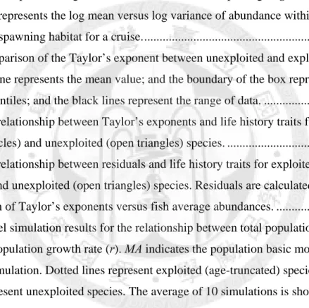
We investigated the spatial mean-variance relationship for each species. Note we considered only the data during the spawning period for a given species (defined in Hsieh et al. 2005). Again, we used larvae distribution to represent the spatial distribution of spawners, and thus we basically explored the spawning aggregation of fishes. First, for each species, we define its principal spawning habitat. To do so, we selected the stations with at least three non-zero records in each species’ spawning period from 1951 to 2007. The minimal polygon encompassing these stations is defined as the principal spawning habitat of that species (see an example in Fig. 1). As such, zero values or occasional occurrence outside the fish’s habitat would not be used to estimate the mean-variance relationship.

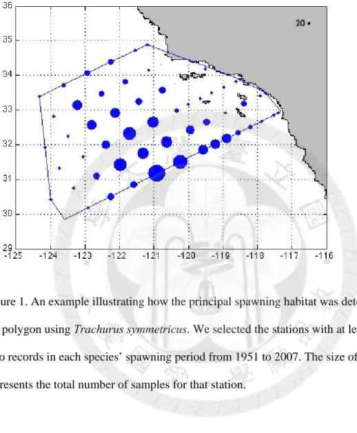
Secondly, we calculated the mean and variance for the fish abundance within this area for each cruise within their spawning period. Thirdly, according to Taylor’s power law, log(V)

= log(a) + b*log(M), we used the ordinary linear regression of log mean versus log variance to obtain the Taylor’s exponent, ‘b’ and intercept ‘a’ (Taylor 1961) (as in Fig. 2).

The Taylor’s exponent and intercept of each species is shown in Table 1. One may consider potential seasonal variation in Taylor’s exponent for a species. Therefore, we have also calculated Taylor’s exponent separately for each season, but we found that there is no significant difference between the values from different seasons (repeated measured ANOVA, p>0.05). Therefore, we included the data for all cruises within the species’

spawning period for later analyses.

The influence of life history traits and fishing impact on Taylor’s exponent

To estimate the influence of life history traits and fishing on Taylor’s exponent (TE), we used the general linear model (Kutner et al. 2005) for each trait (life) and considered the exploitation status as a dummy variable (fishing). For each model, we included mean abundance as a covariate (abun), because abundance was found to correlate with Taylor’s exponent and intercept in our analyses, and such a relationship has been shown in previous statistical theory (Engen 2008). We investigated the following four models:

Model 1: TE = β0 + β1life + β2fishing + β3abun (1) The first model includes three variables: life, fishing, and abun. For the life term, we tested each trait separately to examine whether a relationship exists between TE and trait values.

We set a dummy variable fishing (i.e. exploited: 1; unexploited: 0) to test the fishing impacts.

Model 2: TE = β0 + β1life + β2abun + β3life × fishing (2) The second model tests whether a significant difference exists between the regression slopes (TE versus trait) estimated from the exploited and unexploited fishes. To do so, we include the interaction term life × fishing. This test is again done for each trait separately.

Model 3: TE = β₀ + β₁life + β₂fishing + β₃abun + β₄life × fishing (3) The third model takes both fishing effect itself and the interaction of fishing and life history traits into consideration. It is a combination of model 1 and 2.

Model 4: TE = β₀ + β₁life + β₂fishing + β₃abun + β₄life × fishing + β₅abun × fishing (4)

For testing whether fishing will influence the abundance of exploited species, we include the forth model considering the fishing effect on abundance using an interaction term of fishing x abun. It tests for each trait separately as well.

Individual Based Model

We used an individual-based model to investigate the spatial dynamics of fish by Netlogo (Center for Connected Learning and Computer-Based Modeling, Northwestern University, Evanston, IL). We asked the following questions. First, how could Taylor’s

Power Law be generated? Second, whether and how changes in parameters influence on Taylor’s exponents? Third, does exploited species have high Taylor’s exponent because of age-truncation? We consider a population of a single species living in a continuous environment with 64 x 64 patches (with 10 pixel for each patch). For avoiding boundary effect, we assume the space is like a sphere, which the top and bottom edges of the world are connected and the left and right edges are connected. The space was equally divided into 16 (4 × 4) plots, and two of the plots are defined as ‘good’ habitats while the others are

‘poor’ habitats by setting different mortality rate. We randomly selected two patches as

‘good’ habitats and found no significant effects caused by configuration difference through comparing Taylor’s exponents calculated by every configuration. We used the parameters env to represent the mortality rate. The env is chosen from a uniform random number from 25 to 80 for poor habitats and from 0 to 20 for good habitats. Then, we generated population dynamics with a modified spatial logistic model (Laws et al. 2003). Every individual of the initial population (size = 10) randomly spreads in the environment, with age randomly set from 0 to 5. Each organism xi lives through three events comprising movement, reproducing, and death in every time step.

At the beginning of every time step, an organism starts to reproduce B(xi, x) offspring at site x, which is given by

B(x_i, x) = r × age (5)

where r represents the reproduction rate, and r × age is per capita age-specific fecundity, assuming older fish reproduce more offspring.

A density dependent migration is considered since local population size may affect emigration and immigration rates for some taxa (Bowler and Benton 2005). In the movement step, each individual will sense a patch within a radius of 8 to find a patch containing the most individuals. This assumes that individuals tend to move toward the crowds because the locations of crowds may indicate better habitat nearby. The individual then moves k steps toward the crowd. We assume that an older fish has a bigger body size and thus it should have better moving ability. To model this, k is randomly chosen from a normal distribution N(0, MA×(1＋0.1×age)), in which MA is the basic moving ability set to be the same for the whole population. As the age increases, the moving distance increases.

In the next step, organisms enter the death stage. Individual’s death is determined by the probability function D(xi) that contains both intrinsic death rate and negative density dependence effect given by

0.15    16 0.00003    0.01          

(7) Here, m is the intrinsic per capita death rate, and it is set as 0.5 in our experiment.

Environmental condition is considered as the parameter k, as described above, k is randomly selected from 0 to 20 for a good habitat and 25 to 80 for a bad habitat. Then, global and local negative density effects are both taken into account. The third term represents global negative biomass effect. That is, with the increasing total biomass (ttlage), every individual will suffer a higher mortality simultaneously. We assume that older

individuals have bigger body size thus have higher biomass, so we sum the age of every individual in the space to represent the total biomass. Locally density effect is represented as the forth term, in which d(x) is the total biomass of patch x, and it multiplies with the interaction kernel w(x - xi) to get a weighted pressure for the organism in site xi from its neighborhood at site x. w(x - xi) is given by

w(x  x

)  1 2  ^e

(xx_i² 2 S_w² )

(8) where Sw regulates the competition pressure from neighbors in different distances to xi. When Sw decreases, most of the competition pressure comes only from neighbors near the organism in xi. Sw was set as 1.3 in this study. Moreover, we assume that older individuals have smaller mortality. Thus, we use parameter AS, which is set as 0.003, to describe how much survival rate increases with age. For example, if the death probability for an individual with age 0 is D, for individual with age 1 in the same environment, its death probability will be D-AS. Because older fishes have better adaptability than young fishes especially when the environment condition is bad, we assume the age benefit will be more apparent in poor habitats. After the death phase, every survival individual grows up one year old and moves again.

The model generates a population reaching density capacity after about 20 to 25 generations. We run the model more than 300 time steps, and use the 200 to 300 generations to calculate Taylor’s exponent. For each generation, we measure the abundance of each plot. Then, we obtain the mean and variance of abundance for the whole space.

Next, we used ordinary linear regression of log mean and log variance to estimate Taylor’s exponent ‘b’ according to the equation, log(V) = log(a) + b*log(M). We changed reproduction rate (r) from 5 to 10 and moving ability (MA) from 5 to 9 to investigate their influences on Taylor’s exponent. Ten replicates are simulated for each parameter combination. We also estimated the population growth rate by fitting abundance of the first 100 time steps into logistic growth curve. We hypothesize that Taylor’s exponent increases along with increasing population growth rate and reproduction rate according to Anderson’s model (Anderson et al. 1982). In addition, we hypothesize that the population with a higher moving ability will be more aggregated and thus has a higher Taylor’s exponent.

To test whether fishing will influence Taylor’s exponent through altering species’

demographic processes, we consider age truncation in the model. In such cases, individuals are determined to die after they are older than 3, mimicking age truncation. We define age- truncated species as exploited species, and species with complete age structure represent unexploited species. Our hypothesis for fishing effect is that exploited species may have higher Taylor’s exponent. If so, it will support our inference for real data that exploited species with K-selective traits have higher Taylor’s exponent than unexploited species is because over-fishing changes their demographic traits.

Results

Spatial mean-variance relationship of CalCOFI data

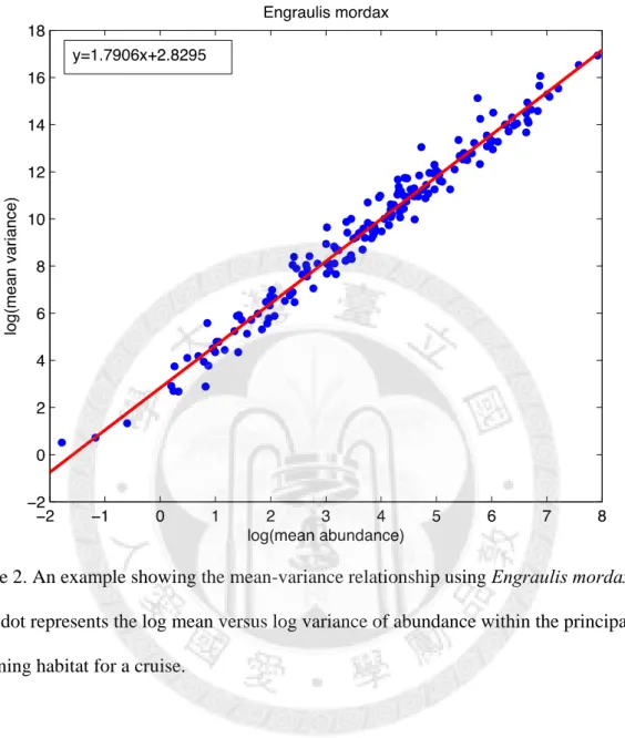
In the CalCOFI area, the exploited species have higher Taylor’s exponents than the unexploited species generally; however, the difference is not significant (p=0.377, Fig. 3).

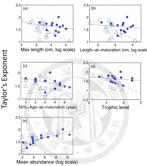
Taylor’s exponents of the unexploited species show a significant linear relationship with maximum length (r = -0.589, p < 0.05, Fig. 4a), length at maturation (r = -0.618, p < 0.05, Fig. 4b), and trophic level (r = -0.582, p < 0.05, Fig. 4d), while the exponents of the exploited species have no statistical significant relationship with any life history trait investigated here (Fig. 4). In addition, we found that Taylor’s exponents have strong correlation with the mean abundance (exploited species: r = 0.808, p < 0.01; unexploited species: r = 0.637, p < 0.01, Fig. 4), and the slope of this linear relationship is also not significant different between exploited and unexploited species (p = 0.675).

The results of general linear models show that model 3 (lowest AIC) best explains the relationship between Taylor’s exponents versus traits, fishing, and mean abundance (Table 2). In model 3, we found that life and abun terms are both significant for all traits. Taylor’s exponents decrease along with species’ traits, but they increase with mean abundances.

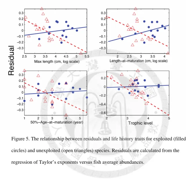
Furthermore, fishing impact and fishing/life trait interaction term is also significant for all traits. The significant interaction term indicates that the negative relationship between life history traits and Taylor’s exponent is weaker or even diminished in exploited species (Table 2). After partial out the effect of abundance, we can see a clearer pattern of different

relationship of Taylor’s exponents versus life history traits between the exploited and unexploited species (Fig. 5).

Individual Based Model

We successfully reproduce Taylor’s power law in most of the simulations. For analyses, we consider only the result when the R² of log mean-variance regression is larger than 0.5.

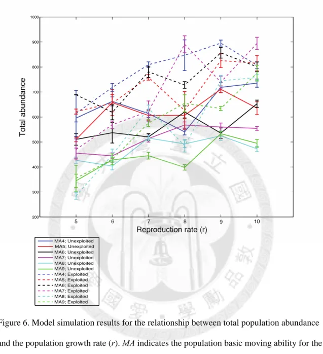
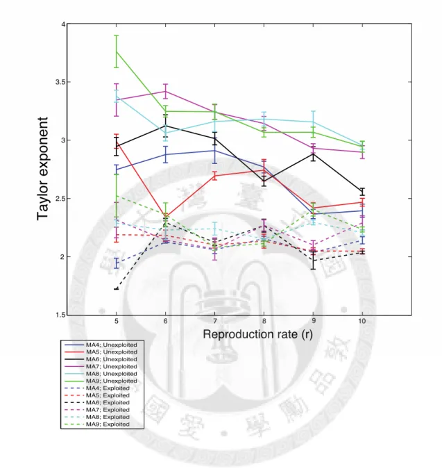
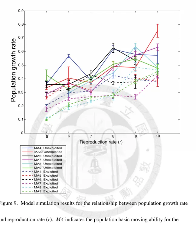
To investigate the impact of demographic factors, we first examine the results of unexploited species. Our simulation indicates that the total population abundance increases with the reproduction rate (r) generally, but exhibits no correlation with species moving ability (Fig. 6). Population growth rates are estimated to be between 0.1 to 0.8, and are correlated to reproduction rates (Fig. 8). However, Taylor’s exponent decreases with population growth rate and reproduction rate (r), which is contrast to our expectation. In addition, species with high moving ability (MA = 7, 8, 9) tend to have bigger Taylor’s exponents than low moving ability species (MA = 4, 5, 6), but there is no obvious trend between Taylor’s exponents and moving abilities within the two group.

We then compare the results between exploited (age-truncated case) and unexploited species to investigate fishing effect. Unexploited species have higher population abundance than exploited species that have the same moving ability and reproduction rate.

Unexploited species also have higher Taylor’s exploited species than age-truncated ones, which is against to our hypothesis and empirical data. Although Taylor’s exponent decreases with reproduction rate (r) in unexploited species, it stays stable when r varies in exploited species (Fig. 7). In comparison with unexploited species, age-truncated species do

not show apparent different Taylor’s exponents among groups with different moving ability, except in the cases of reproduction rate 9 (Fig. 7).

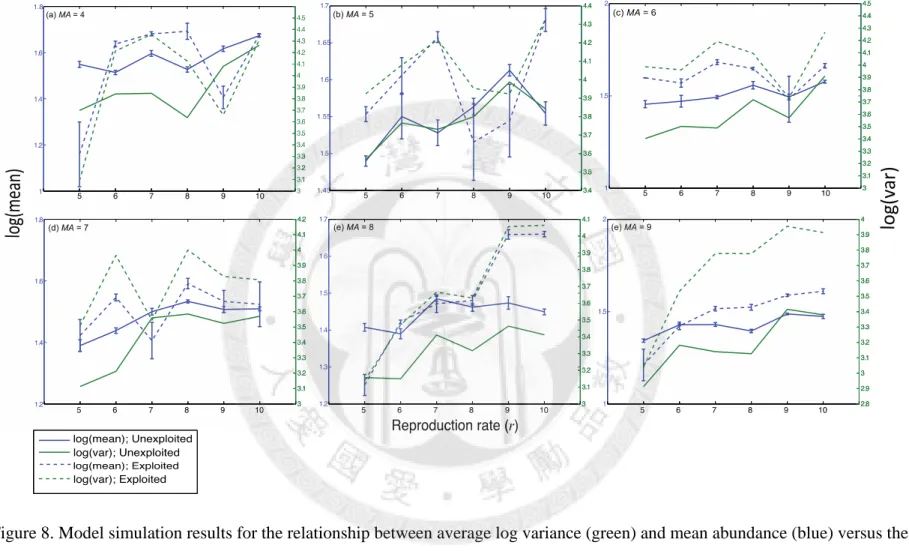
In order to understand how traits influence Taylor’s exponent, we investigated how the average log variance and log mean abundance changes with increasing r and MA, and compared the results of exploited species and unexploited species (Fig. 8). Both variance and mean abundance increase with growth rate (r) and then gradually reach saturation except when MA is 6. For unexploited species, log variance generally goes up with population growth rate faster than log mean. However, we observed Taylor’s exponent decreases with r instead of rising, indicating that growing reproduction rate also raises Taylor’s intercept. This phenomenon happens in unexploited cases more significantly than exploited species. Furthermore, the ratio of average log variance versus log mean of exploited species is higher than unexploited species in every MA categories, suggesting that exploited species in fact have higher variance than unexploited species when their mean abundance is similar, but the variance of unexploited species is more sensitive to the trend of mean abundance, representing as a higher b. It is also noteworthy that log variance and log mean abundance of exploited species are more sensitive to the change of reproduction rate than unexploited species in most of cases, especially when MA is 8 and 9.

Discussion

Spatial mean-variance relationship of CalCOFI data

Our results show a negative relationship between life history traits and Taylor’s exponent (Fig. 4, Table 2), and it is consistent with Anderson’s demographic model (Anderson et al.

1982) that species with r-selected life history traits have higher Taylor’s exponent (Fig. 4).

This comparison across species is valid because several studies have shown that Taylor’s exponent is constant within species under the same condition (e.g. sampling scale, environment, life stage) (Taylor et al. 1988, Nestel 1995, Elliott 2004). Although Anderson did not explain why r-selected species have higher Taylor’s exponent than K-species, the negative relationship between traits and b may be explained by several possible mechanisms. Firstly, species with r-selective traits are small body size organisms, indicating relatively low migration ability than species with K-selected traits. This positive relationship between body size (or mass) and dispersal distance is also found in many active dispersal organisms, including beetles, birds, and whales (Peters 1986, Jenkins et al.

2007). Therefore, a species with small body size may have poor dispersal ability thus being less aggregated. Secondly, species with K-selected traits have better ability to buffer environmental stress than r-selective species (Smith 1954, Pianka 1970). K-selected species can reduce environmental challenge in many ways; for instance, large organisms have fewer predators and more types of prey (Pianka 1970). As a result, species with K- selected traits are more likely to spread in different habitat types and thus have a more balanced distribution in space and thus a lower Taylor’s exponent. Thirdly, r-selected species have high population growth rate due to their short generation time and high

fecundity (Pianka 1970). As a consequence, r-selected species could have higher local density than K-selected ones in spawning season. The facts that we find empirical relationships between Taylor’s exponents versus life history traits indicate that Taylor’s power law can be explained by biological mechanisms. This is contrast with previous studies that suggest that Taylor’s power law is resulted from statistical invariant as explained by statistical theory of error (Kendal 2004).

We found that exploited species have higher Taylor’s exponents, especially in the species with traits more similar as K-selective strategy (Fig. 4). This conclusion remains hold after partial out the effects of abundance (Fig. 5). We considered two possible ways that fishing can elevate Taylor’s exponent: decreasing population abundance and thus increasing the population’s spatial variation (Basin Model, Maccall 1990), and/or altering species demographic processes through age-truncation. Although these two mechanisms cannot easily be separated, the result we found suggesting that the second influence (altered demographic process) may be more adequate to explain our observation. Basin model suggested that population will shrink into their best habitat when the abundance decline.

However, we found that exploited and unexploited species have similar mean abundance (Fig. 11) and average Taylor’s exponents (Fig. 1), indicating that fishing has not change fishes spatial pattern through decreasing population abundance. Nevertheless, we found that Taylor’s exponents of unexploited species exhibit a stronger relationship with life history traits than exploited species (Table 2, Fig. 4). If only the population abundance decline happened, we would observe the negative trend between traits and Taylor’s exponent panning up without changing the slope. Therefore, we suggest that fishing may have altered

the traits of exploited species, making them behave like r-selective species. As a result, the exploited species exhibits a higher variance in spatial distribution than unexploited species with the same abundance and recorded life traits. Our finding is also consistent with previous research that fishing reduced spatial heterogeneity of exploited species, likely due to age truncation (Hsieh 2008).

We found that Taylor’s exponents show a strong positive relationship with mean abundance. This phenomenon has also been predicted by theoretical model and observed in empirical data (Hanski 1982, 1987, Hanski and Woiwod 1993). The only one empirical reference of the positive correlation between spatial Taylor’s exponents and mean abundance is stated in Hanski’s (1987) study, in which he compiled some moth and aphid data and found mean abundance is positive correlated with b. Engen et al. (Engen 2008) suggested a mechanism of this positive, linear relationship between Taylor’s exponents and log mean values by a point process model. If the sampling unit is small, strong spatial autocorrelation will make the variance (V) approximate to the function of mean (m):

(9) where v is an overdispersion function, which is approximately constant over small area. cv

represents the coefficient of variance for density in this area. According to equation 9, the first term will be dominant and cause Taylor’s exponent ( ) be about one when the

value of mean is small (ln(m)  0). With ln(m) getting bigger, Taylor’s exponent is approaching 2.

We also found a significant negative effect of the fishing term in the model 3, but it is a statistical result rather than having any ecological meaning. As can be seen in model 1, fishing term is positive but nonsignificant, indicating exploited species have slightly higher Taylor’s exponent. The negative fishing term occurs only after we considered the covariate – life history traits’ influence. Because we set the dummy variable fishing as 1 in model 3, fishing × life actually equals to life for exploited species. Therefore, Taylor’s exponents of exploited species were explained by traits twice. As a result, the residuals of b from regressed with abun and fishing × life of exploited species will have a more positive slope than unexploited species while regressed with life again. This forces a smaller intercept of the regression residuals versus life in exploited species, and thus we get a negative coefficient of fishing (Fig. S1).

Individual Based Model

We used individual-based model to investigate how life history traits and fishing influence Taylor’s exponent. Our model shows that Taylor’s Power Law can be generated under some simple demographic processes with environmental heterogeneity and density dependence migration (Hanski 1987, Perry 1988). Then, we tested Anderson’s model that species with r-selected traits, such as small body size (i.e. less moving ability) and high population growth rate, have bigger Taylor’s exponent than species with K-selected traits.

Firstly, we found Taylor’s exponents decrease with reproduction rate (r) and population growth rate (Fig. 7, 10), which is opposite to our hypothesis. One possible reason may be the spilling effect while abundance increases. Occupied area will increase with abundance

increasing (MacCall 1990, Swain and Sinclair 1994) because of the competition pressure of the central of original habitat, thus individuals may increase utilization of the neighboring area. Consequently, Taylor’s exponents will decrease with occupancy (Yamamura 2000).

However, we observed that the average variance actually increases with reproduction rate, suggesting the lower b owing Taylor’s intercept, a, increases with reproduction rate. That is, with reproduction rate getting high, the local density increases so quickly that high variance can be observed no matter how the mean abundance is. Secondly, species with higher moving ability (MA = 7, 8, 9) tend to have bigger Taylor’s exponents than those with lower MA (MA = 4, 5, 6). Furthermore, the simulations with high moving ability sometimes generated the exponents of Taylor’s Power law larger than 2, which is seldom observed in others’ simulation results (Iwao 1968, Hanski 1980, Anderson et al. 1982, Hanski 1982).

Although those larger b values observed in real data may be caused by sampling issue (Taylor et al. 1980, Yamamura 2000), positive congregation may be a better explanation for the big Taylor’s exponents in our simulations (Taylor et al. 1983). In our model, individual will turn toward the place with the highest density in its neighborhood, because the most crowded area indicates its good condition for living. We should note that this situation not always happens in real world, especially when the place reaches its carrying capacity. In such condition, individuals may tend to other places to seek for more resource and less competition.

We found that exploited (age-truncated) species have lower Taylor’s exponent than unexploited species. However, exploited species have bigger ratio of average log variance and log mean abundance than unexploited species, indicating that instead of influence the slope of mean-variance relationship as empirical data, age-truncation alters the spatial

pattern by raising the intercept in our model. That is, exploited species generally have higher spatial variance, but their simple age structure makes them lost the plasticity of changing spatial pattern with abundance changes. In CalCOFI data, we also found that species with r-selected traits, show a slight Taylor’s exponent change, have a higher intercept than unexploited species (Fig. S2), though it is not statistical significant. In contrast to Taylor’s exponents, there is only a few study mentioned about the intercept, and the meaning of intercept also remains elusive. Taylor firstly stated that the intercept (a) is just a sampling or computing factor which has no particular biological meaning (Taylor 1961), but then he found that some bird species show constant b among different environments with their a varies (Taylor et al. 1983). Our results show that Taylor’s intercept may also be influenced by demographic process even in the same environment.

Such results indicate that species spatial pattern may be influenced in several ways.

There are also some caveats in our model need to be improved. At first, the population dynamic we generated is not a perfectly smooth logistic growth. That is, even we can observe a logistic growth curve, there are still some fluctuations happen when the population abundance is about to saturate. Furthermore, we only consider the time series when temporary variation is stationary, but lack of examining oscillation or chaos situations.

How such dynamic pattern affects the spatial Taylor’s power law is a subject for further analysis.

To sum up, our empirical result is consistent with Anderson’s model that r-selective species have higher Taylor’s exponents, though the simulation does not support

exponent. Nevertheless, we still can observe the spatial variance increases with reproduction rate in the model result. This difference between empirical data and simulation result also occurs in the comparison of exploited and unexploited species.

Although exploited species show a more aggregated pattern, it reflects on turning up the exponents in real data, but increases average spatial variance-mean ratio in the model. This kind of reduced spatial heterogeneity may weaken the adaptability to environmental change in exploited species. Thus, a sound fishery management should concern age and spatial structure of exploited fishes.

References

Anderson, R. M., D. M. Gordon, M. J. Crawley, and M. P. Hassell. 1982. Variability in the abundance of animal and plant-species. Nature 296:245-248.

Ballantyne, F. and A. J. Kerkhoff. 2005. Reproductive correlation and mean-variance scaling of reproductive output for a forest model. Journal of Theoretical Biology 235:373-380.

Ballantyne, F. and A. J. Kerkhoff. 2007. The observed range for temporal mean-variance scaling exponents can be explained by reproductive correlation. Oikos 116:174-180.

Berkeley, S. A. 2004. Maternal age as a determinant of larval growth and survival in a marine fish, Sebastes melanops. Ecology 85:1258.

Blanchard, J. L. 2005. Distribution-abundance relationships for North Sea Atlantic cod (Gadus morhua): observation versus theory. Canadian Journal of Fisheries and Aquatic Sciences 62:2001.

Boag, B., C. A. Hackett, and P. B. Topham. 1992. The use of Taylor power law to describe the aggregated distribution of gastrointestinal nematodes of sheep. International Journal for Parasitology 22:267-270.

Bohlin, T. 1977. Habitat Selection and Intercohort Competition of Juvenile Sea-Trout Salmo trutta. Oikos 29:112-117.

Bowler, D. E. and T. G. Benton. 2005. Causes and consequences of animal dispersal strategies: relating individual behaviour to spatial dynamics. Biological Reviews 80:205-225.

Cottingham, K. L., B. L. Brown, and J. T. Lennon. 2001. Biodiversity may regulate the temporal variability of ecological systems. Ecology Letters 4:72-85.

Crecco, V. and W. J. Overholtz. 1990. Causes of Density-Dependent Catchability for Georges Bank Haddock Melanogrammus aeglefinus. Canadian Journal of Fisheries and Aquatic Sciences 47:385-394.

Downing, J. A. 1986. Spatial heterogeneity: evolved behaviour or mathematical artefact?

Nature 323:255.

Elliott, J. M. 2004. Contrasting dynamics in two subpopulations of a leech metapopulation over 25 year-classes in a small stream. Journal of Animal Ecology 73:272-282.

Engen, S. 2008. A general model for analyzing Taylor's spatial scaling laws. Ecology 89:2612.

Hanski, I. 1980. Spatial patterns and movements in coprophagous beetles. Oikos 34:293.

Hanski, I. 1982. On patterns of temporal and spatial variation in animal populations.

Annales Zoologici Fennici 19:21-37.

Hanski, I. 1987. Cross-correlation in population-dynamics and the slope of spatial variance- mean regressions. Oikos 50:148-151.

Hanski, I. and J. Tiainen. 1989. Bird ecology and Taylor variance-mean regression.

Annales Zoologici Fennici 26:213-217.

Hanski, I. and I. P. Woiwod. 1993. Mean-related stochasticity and population variability.

Oikos 67:29-39.

Heino, M. 1998. Management of evolving fish stocks. Canadian Journal of Fisheries and Aquatic Sciences 55:1971.

Hsieh, C. 2006. Fishing elevates variability in the abundance of exploited species. Nature 443:859.

Hsieh, C. H., C. Reiss, W. Watson, M. J. Allen, J. R. Hunter, R. N. Lea, R. H. Rosenblatt, P.

E. Smith, and G. Sugihara. 2005. A comparison of long-term trends and variability

in populations of larvae of exploited and unexploited fishes in the Southern California region: A community approach. Progress in Oceanography 67:160-185.

Hsieh, C. H., C. S. Reiss, R. P. Hewitt, and G. Sugihara. 2008. Spatial analysis shows that fishing enhances the climatic sensitivity of marine fishes. Canadian Journal of Fisheries and Aquatic Sciences 65:947-961.

Hsieh, C. H., A. Yamauchi, T. Nakazawa, and W. F. Wang. 2010. Fishing effects on age and spatial structures undermine population stability of fishes. Aquatic Sciences 72:165-178.

Iwao, S. i. 1968. A new regression method for analyzing the aggregation pattern of animal populations. Researches on Population Ecology 10:1-20.

Jenkins, D. G., C. R. Brescacin, C. V. Duxbury, J. A. Elliott, J. A. Evans, K. R. Grablow, M. Hillegass, B. N. Lyon, G. A. Metzger, M. L. Olandese, D. Pepe, G. A. Silvers, H.

N. Suresch, T. N. Thompson, C. M. Trexler, G. E. Williams, N. C. Williams, and S.

E. Williams. 2007. Does size matter for dispersal distance? Global Ecology and Biogeography 16:415-425.

Jennings, S. and N. K. Dulvy. 2005. Reference points and reference directions for size- based indicators of community structure. ICES Journal of Marine Science: Journal du Conseil 62:397-404.

Jennings, S. and M. J. Kaiser. 1998. The effects of fishing on marine ecosystems. Pages 201-+ Advances in Marine Biology, Vol 34. Academic Press Ltd, London.

Jorgensen, C., B. Ernande, and O. Fiksen. 2009. Size-selective fishing gear and life history evolution in the Northeast Arctic cod. Evolutionary Applications 2:356-370.

Kendal, W. S. 2004. Taylor's ecological power law as a consequence of scale invariant

Kutner, M. H., C. J. Nachtsheim, J. Neter, and W. Li. 2005. Applied linear statistical models. McGraw Hill International eddition.

MacCall, A. D. 1990. Dynamic geography of marine fish populations. University of Washington Press, Seattle, Washington.

Marshall, C. T. 1995. Density-dependent habitat selection by juvenile haddock (Melanogrammus aeglefinus) on the southwestern Scotian Shelf. Canadian Journal of Fisheries and Aquatic Sciences 52:1007.

Murawski, S. A. 2001. Impacts of demographic variation in spawning characteristics on reference points for fishery management. ICES Journal of Marine Science 58:1002.

Nestel, D. 1995. Spatial distribution of scale insects: comparative study using Taylors power law. Environmental Entomology 24:506.

Perry, J. N. 1988. SOME MODELS FOR SPATIAL VARIABILITY OF ANIMAL SPECIES. Oikos 51:124-130.

Peters, R. 1986. The ecological implications of body size. Cambridge University Press, Cambridge.

Pianka, E. R. 1970. On r- and K-Selection. The American Naturalist 104:592-597.

Rose, G. A., B. deYoung, D. W. Kulka, S. V. Goddard, and G. L. Fletcher. 2000.

Distribution shifts and overfishing the northern cod (Gadus morhua): a view from the ocean. Canadian Journal of Fisheries and Aquatic Sciences 57:644-663.

Smith, F. E. 1954. Quantitative aspects of population growth. Dynamics of growth processes:277-294.

Stoner, A. W. and A. A. Abookire. 2002. Sediment preferences and size-specific distribution of young-of-the-year Pacific halibut in an Alaska nursery. Journal of Fish Biology 61:540-559.

Swain, D. P. and A. F. Sinclair. 1994. Fish Distribution and Catchability: What Is the Appropriate Measure of Distribution? Canadian Journal of Fisheries and Aquatic Sciences 51:1046-1054.

Swain, D. P. and E. J. Wade. 1993. Density-Dependent Geographic Distribution of Atlantic Cod (Gadus morhua) in the Southern Gulf of St. Lawrence. Canadian Journal of Fisheries and Aquatic Sciences 50:725-733.

Taylor, L. R. 1961. Aggregation, variance and mean. Nature 189:732-&.

Taylor, L. R. 1986. Synoptic dynamics, migration and the Rothamsted insect survey:

Presidential address to the British Ecological Society, December 1984. Journal of Animal Ecology 55:1.

Taylor, L. R., J. N. Perry, I. P. Woiwod, and R. A. J. Taylor. 1988. Specificity of the spatial power-law exponent in ecology and agriculture. Nature 332:721-722.

Taylor, L. R. and R. A. Taylor. 1977. Aggregation, migration and population mechanics.

Nature 265:415-421.

Taylor, L. R., R. A. J. Taylor, I. P. Woiwod, and J. N. Perry. 1983. Behavioural dynamics.

Nature 303:801-804.

Taylor, L. R., I. P. Woiwod, and J. N. Perry. 1980. Variance and the Large Scale Spatial Stability of Aphids, Moths and Birds. Journal of Animal Ecology 49:831-854.

Taylor, R. A. J. 1981a. The Behavioural Basis of Redistribution I. The Delta-Model Concept. Journal of Animal Ecology 50:573.

Taylor, R. A. J. 1981b. The Behavioural Basis of Redistribution. II. Simulations of the Delta-Model. Journal of Animal Ecology 50:587.

Tilman, D. 1999. The ecological consequences of changes in biodiversity: a search for

Winters, G. H. and J. P. Wheeler. 1985. Interaction Between Stock Area, Stock Abundance, and Catchability Coefficient. Canadian Journal of Fisheries and Aquatic Sciences 42:989-998.

Yamamura, K. 2000. Colony expansion model for describing the spatial distribution of populations. Researches on Population Ecology 42:161.

圖目錄

Figure 1. An example illustrating how the principal spawning habitat was determined by the polygon using Trachurus symmetricus. We selected the stations with at least three non-zero records in each species’ spawning period from 1951 to 2007. The size of filled circles represents the total number of samples for that station. ... 31 Figure 2. An example showing the mean-variance relationship using Engraulis mordax.

Each dot represents the log mean versus log variance of abundance within the

principal spawning habitat for a cruise. ... 32 Figure 3. Comparison of the Taylor’s exponent between unexploited and exploited species.

The red line represents the mean value; and the boundary of the box represent 25^th and 75^th percentiles; and the black lines represent the range of data. ... 33 Figure 4. The relationship between Taylor’s exponents and life history traits for exploited

(filled circles) and unexploited (open triangles) species. ... 34 Figure 5. The relationship between residuals and life history traits for exploited (filled

circles) and unexploited (open triangles) species. Residuals are calculated from the regression of Taylor’s exponents versus fish average abundances. ... 35 Figure 6. Model simulation results for the relationship between total population abundance

and the population growth rate (r). MA indicates the population basic moving ability for the simulation. Dotted lines represent exploited (age-truncated) species, while solid lines represent unexploited species. The average of 10 simulations is shown with standard error. ... 36 Figure 7. Model simulation results for the relationship between Taylor’s exponents and the

population growth rate (r). MA indicates the population basic moving ability for the simulation. Dotted lines represent exploited (age-truncated) species, while solid lines represent unexploited species. The average of 10 simulations is shown with standard error. ... 37 Figure 8. Model simulation results for the relationship between average log variance (green)

and mean abundance (blue) versus the population growth rate (r). Dotted lines

represent exploited (age-truncated) species, while solid lines represent unexploited species. The average of 10 simulations is shown with standard error ... 38 Figure 9. Model simulation results for the relationship between population growth rate and

reproduction rate (r). MA indicates the population basic moving ability for the simulation. Dotted lines represent exploited (age-truncated) species, while solid lines represent unexploited species. The average of 10 simulations is shown with standard error. ... 39 Figure 10. Model simulation results for the relationship between population growth rate and

Taylor’s exponent (b for exploited (filled circles) and unexploited (open triangles) species. ... 40 Figure 11. Comparison of the abundance between unexploited and exploited species. The

red line represents the mean value; and the boundary of the box represent 25^th and 75^th percentiles; and the black lines represent the range of data. Outliers are represented as red crosses. ... 41

Figure 1. An example illustrating how the principal spawning habitat was determined by the polygon using Trachurus symmetricus. We selected the stations with at least three non- zero records in each species’ spawning period from 1951 to 2007. The size of filled circles represents the total number of samples for that station.

Figure 2. An example showing the mean-variance relationship using Engraulis mordax.

Each dot represents the log mean versus log variance of abundance within the principal spawning habitat for a cruise.

Figure 3. Comparison of the Taylor’s exponent between unexploited and exploited species.

The red line represents the mean value; and the boundary of the box represent 25^th and 75^th percentiles; and the black lines represent the range of data.

Figure 4. The relationship between Taylor’s exponents and life history traits for exploited (filled circles) and unexploited (open triangles) species.

Figure 5. The relationship between residuals and life history traits for exploited (filled circles) and unexploited (open triangles) species. Residuals are calculated from the regression of Taylor’s exponents versus fish average abundances.

Figure 6. Model simulation results for the relationship between total population abundance and the population growth rate (r). MA indicates the population basic moving ability for the simulation. Dotted lines represent exploited (age-truncated) species, while solid lines represent unexploited species. The average of 10 simulations is shown with standard error.

Figure 7. Model simulation results for the relationship between Taylor’s exponents and the population growth rate (r). MA indicates the population basic moving ability for the simulation. Dotted lines represent exploited (age-truncated) species, while solid lines represent unexploited species. The average of 10 simulations is shown with standard error.

Figure 8. Model simulation results for the relationship between average log variance (green) and mean abundance (blue) versus the population growth rate (r). Dotted lines represent exploited (age-truncated) species, while solid lines represent unexploited species.

The average of 10 simulations is shown with standard error

Figure 9. Model simulation results for the relationship between population growth rate and reproduction rate (r). MA indicates the population basic moving ability for the simulation. Dotted lines represent exploited (age-truncated) species, while solid lines represent unexploited species. The average of 10 simulations is shown with standard error.

Figure 10. Model simulation results for the relationship between population growth rate and Taylor’s exponent (b for exploited (filled circles) and unexploited (open triangles) species.

Figure 11. Comparison of the abundance between unexploited and exploited species.

The red line represents the mean value; and the boundary of the box represent 25^th and 75^th percentiles; and the black lines represent the range of data. Outliers are represented as red crosses.

表目錄

Table 1.  Taylor’s exponent and intercept of 29 coastal fishes... 43  Table 2. Results of the four general linear models relating the Taylor’s exponent 

with each life history (max size, size at maturation, age at maturation, and trophic  level), abundance, and exploitation status (exploited or not). ... 44 

Table 1. Taylor’s exponent and intercept of 29 coastal fishes

Species Taylor’s exponent Taylor’s intercept

Exploited Engraulis mordax 1.791 2.830

Merluccius productus 2.010 1.920

Microstomus pacificus 1.742 3.362

Paralabrax clathratus 1.766 2.997

Paralichthys californicus 1.693 2.872

Parophrys vetulus 1.263 2.011

Sardinops sagax 1.392 2.370

Scomber japonicus 1.873 1.880

Scorpaenichthys marmoratus 1.390 2.171

Sebastes aurora 1.032 1.433

Sebastes paucispinis 1.448 2.217

Sphyraena argentea 1.257 1.963

Trachurus symmetricus 1.533 2.213

Unexploited Argentina sialis 1.680 2.046

Chromis punctipinnis 1.610 2.231

Cololabis saira 1.482 1.431

Hippoglossina stomata 1.394 2.204

Hypsoblennius jenkins 1.662 2.484

Icichthys lockingtoni 1.757 1.754

Leuroglossus stilbius 1.712 2.450

Lyopsetta exilis 1.168 1.399

Ophidion scrippsae 1.634 2.203

Oxylebius pictus 1.856 2.273

Pleuronichthys verticalis 1.487 1.795

Sebastes jordani 1.408 1.874

Symphurus atricaudus 1.603 2.413

Tetragonurus cuvieri 1.769 2.062

Trachipterus altivelis 1.703 1.537

Zaniolepis frenata 1.082 1.447

Table 2. Results of the four general linear models relating the Taylor’s exponent with each life history (max size, size at maturation, age at maturation, and trophic level), abundance, and exploitation status (exploited or not).

Model 1 TE = β0 + β1life + β2fishing + β3abun

Estimate Error t value Pr > |t| AIC

Intercept 1.694 0.245 6.92 <0.001*** -13.843

Max size -0.123 0.062 -1.99 0.057

Fishing 0.101 0.088 1.15 0.262

Abundance 0.065 0.016 4.01 <0.001***

Estimate Error t value Pr > |t| AIC

Intercept 1.548 0.228 6.80 <0.001*** -12.037

Size at maturation_ -0.103 0.069 -1.49 0.149

Fishing 0.071 0.089 0.80 0.430

Abundance 0.066 0.017 3.80 <0.001***

Estimate Error t value Pr > |t| AIC

Intercept 1.311 0.131 10.03 <0.001*** -10.286

Age at maturation -0.026 0.033 -0.79 0.437

Fishing 0.026 0.085 0.30 0.765

Abundance 0.070 0.018 3.95 <0.001***

Estimate Error t value Pr > |t| AIC

Intercept 1.543 0.274 6.05 <0.001*** -12.463

Trophic level -0.122 0.075 -1.62 0.118

Fishing 0.037 0.076 0.49 0.629

Abundance 0.069 0.016 4.24 <0.001***

Model 2 TE = β0 + β1life + β2abun + β3life × fishing

Estimate Error t value Pr > |t| AIC

Intercept 1.774 0.252 7.05 <0.001*** -14.975

Max size -0.146 0.064 -2.27 0.032*

Max size × Fishing 0.032 0.021 1.54 0.137

Abundance 0.064 0.016 4.04 <0.001***

Estimate Error t value Pr > |t| AIC

Intercept 1.638 0.233 7.02 <0.001*** -13.347

Size at maturation -0.135 0.073 -1.86 0.074

Size at maturation × Fishing

0.036 0.027 1.35 0.188

Abundance 0.063 0.017 3.79 <0.001***

Estimate Error t value Pr > |t| AIC

Intercept 1.370 0.135 10.16 <0.001*** -11.683

Age at maturation -0.054 0.040 -1.35 0.189