行政院國家科學委員會專題研究計畫成果報告
應用數位訊號單晶片於線上適應性控制器之研究 Development of Adaptive In-Line Controller
by Digital Signal Processor
計畫類別:;個別型計畫 整合型計畫 計畫編號:NSC 92-2212-E-006-009
執行期間:90 年 8 月 1 日至 93 年 7 月 31 日 個別型計畫:計畫主持人: 楊世銘 共同主持人:
整合型計畫:總計畫主持人:
子計畫主持人:
處理方式:; 可立即對外提供參考 一年後可對外提供參考 兩年後可對外提供參考
(必要時,本會得展延發表時限)
執行單位: 成功大學航空太空研究所 中華民國 93 年 7 月 31 日
目錄
中文摘要 2
英文摘要 4
1 Motivation 6
2 Algorithm Development 10
2.1 Filtered-X LMS Algorithm 10 2.2 Feedback Controller in Feedforward Algorithm 13 2.3 ARX System Identification Model 16
3 Experimental Design 21
4 Software, Hardware and Firmware 25 5 Experiments of Noise and Vibration Control by a DSP
Controller
33
6 Summary 35
References 38
應用數位訊號單晶片於線上適應性控制器之研究 中文摘要
主動式噪音與振動控制技術已發展至實際系統工程之應用。傳統進行適應性 噪音與振動控制至少需要兩個以上的感測器,一為量測噪音或振動之參考源感測 器,另一為量測噪音或振動控制後之誤差感測器。然而一般參考源是難於量測 的。因此本計畫提供一有效的方法應用單一感測器進行適應性噪音與振動控制。
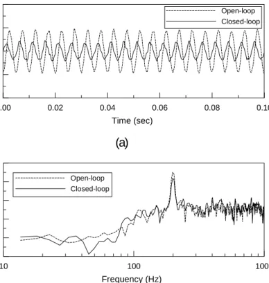
藉由應用 TMS320C31 數位訊號處理器於適應性濾波器與 Filtered-X LMS 調變法 則之實現,管路及噪音控制耳機之噪音控制實驗有顯著之控制效果。實驗之參 數,諸如:取樣率、控制器階數、系統識別之階數和調變收斂率,本計畫亦提供 一有效之實驗計畫法,以獲得最佳參數選擇。實驗結果顯示此單一感測器方法可 有效降低低頻之噪音與振動。並且藉有 TMS320C31 與 EPROM 之設計,本計畫發展 之獨立運作之數位訊號處理控制器,可有效轉移主動式噪音控制至實際系統工程 之應用。
第一年計劃發展應用單組感測器與致動器之適應性控制器的設計與分析。
此控制器有別於現今適應性濾波器需要多組感測器或需有參考訊號。此計畫發展 之適應性控制器將以ARX或ARMA為線上系統識別,另以FXLMS為計算法則用以設計 線上適應性控制器。在時程與經費的考量下,以一個一維管路模型模擬簡化飛機 機艙模型噪音控制為載具,驗證此控制器之設計,以個人電腦判別系統之噪音頻 譜,應用音圈式致動器和麥克風元件感測器配合TI-TMS320C32數位訊號板進行噪 音控制,以降低來自引擎之低頻諧振噪音。實驗結果用以設計實用之適應性控制 器,藉適當頻寬與即時運算能力以有效應用於實際減振與減噪系統。
第二年計劃著重應用實驗計畫法進行適應性控制器之參數最佳化設計,並 於前述實驗模型中以驗證其成效。另以TI-TMS320C32數位訊號板為例研究如何匹 配適當系統識別器階數、濾波器階數與其計算法則。主動式線上適應性控制之設
計成敗端賴如何有效整合系統動態特性,感測器與致動器特性和控制晶片之特 性。
第三年計劃則致力於單機操作之適應性控制器研究並研發一單機操作之數 位訊號處理器(即毋需PC)為基礎之控制器,以取其輕薄短小且低耗電率之優點。
由模型識別,信號量測,和數位訊號控制器設計,將可建立一完整且可行之設計 工具與流程,並以減噪和減振系統為例,以應用於實際工程系統之適應性控制器。
應用適應性濾波器原理之主動式適應性控制乃結合系統線上識別、線上控制 與數位訊號處理之一項實用技術,計劃成果除可直接應用航空器上,亦可於實際 相關產業如高鐵、汽機車和大哥大通訊等。
Development of Adaptive In-Line Controller by Digital Signal Processor
Abstract
The technology of active noise and vibration control has been in practical implementation. Conventional adaptive noise and vibration control systems often utilize several sensors: at least one to measure the reference input or disturbance source while another one to measure the attenuated noise or residual vibration signal.
However, it is often difficult to measure only the disturbance source. A simple and effective configuration by using only one sensor for adaptive noise control is developed in this project. The controller of a finite impulse response (FIR) adaptive filter is by using the filtered-X LMS algorithm implemented in a TMS320C31 digital signal processor (DSP). Analyses and experiments of adaptive noise control in duct and headset are conducted to validate the controller design. The system parameters:
the sampling rate, the dimension of the controller, the dimension of the secondary path model identification and the convergence rate, are analyzed by experimental design. Experiments show that this single sensor/actuator configuration can effectively attenuated the low-frequency noise and vibration. A standalone controller implemented on TMS320C31 digital signal processor (DSP) with external boot erasable programmable read only memory (EPROM) is also developed to facilitate the transition from laboratory experiments to engineering applications.
1. The first year program has developed an adaptive control system by using only a pair of sensor and actuator. Microphone and voice-coil speaker, as sensor/actuator, with a PC-based TI-TMS320C32 digital signal processor board are employed in the initial phase of a simplified aircraft cabin model in suppressing the low frequency harmonic noises. The noise control experiment results have validated the adaptive
controller configuration and facilitated the development of active noise control headset of desired bandwidth in the second year program.
2. The second year program has integrated the experimental design method and the adaptive controller design so as to optimize the parameters of system identification order and controller order. The sensor/actuator/controller are then applied in noise control experiment of an active noise control headset. Control spillover has been prevented for effective implementation of the digital signal processor.
3. The third year program has also implemented the adaptive control algorithm into a standalone programmable digital signal processor. By integrating (1) the system identification of the acoustic model, (2) the noise signal measurement, and (3) digital signal processing controller, this adaptive control system can be implemented in aircraft for noise control and suppression.
Adaptive controller design based on adaptive filter combines the technologies in engineering system on-line identification, control computation algorithm, and digital signal processor. This adaptive controller development tool is expected to be very promising not only in aircraft cabin noise and vibration suppression but also in bullet train, automobile, and motorcycle, and mobile communication systems.
1. Motivation
Noise control has been receiving increasing interests in recent years for it can be applied in a number of engineering systems. The techniques employed can usually be passive absorption and/or active noise control, depending on the practical situation of interest. Passive noise control utilizes the absorption property of matter by mounting sound-absorbent materials on and/or around noise source. This technique has been proven to be cost-effective at higher frequencies. For lower frequencies, however, the bulk of the absorbent materials required, and the cost of necessary hardware, increases exponentially. This, further, leads to maintenance problems, making passive techniques impractical for low-frequency noise reduction.
Active noise control (ANC) uses the intentional superposition of acoustic waves to create a destructive interference pattern for reduction of the unwanted noise. This is realized by a single or a number of secondary acoustics sources, driven by electrical signals derived from the primary (unwanted) noise through detection sensors and electronic controller(s). When acoustic waves are superimposed upon one another, they interfere destructively and reduction of the sound occurs. Such stable destructive interference pattern is effective at low frequencies because the computations required for on-line control at high frequencies are much more demanding. This limitation of frequency range and control bandwidth is complementary to that of passive noise control. Practical solution may require a combination of passive techniques for higher frequencies and active techniques for low frequencies.
Conventional noise control systems often utilize several sensors: at least one to measure the noise field and another one to measure the attenuated noise. The sensor, however, gives a combined measure of the noise and the reflected components from the secondary path. Since sensor microphone can not distinguish between the noise
and the reflected components, this causes the so-called “acoustic feedback” problem and often leads to system instability and/or little noise reduction. In addition, engineering practice requires not only continuous and reliable measurement but also fast signal processing. The actuator (anti-phase noise source) must be located near the noise source or the receiver. If their relative positions change, their phase difference will be shifted accordingly that may lead to reinforcement rather than cancellation effect. A simple and yet effective adaptive controller configuration for active noise control is hence necessary.
Sound wave can propagate through both air path and structure path so that active noise control can be conducted by controlling air-borne noise and/or structure-borne noise. Active (air-borne) noise control is achieved by superposing an anti-phase noise on the unwanted one in order to cancel the sound field in the desired zone.
This simple principle was first recognized by Lueg (1936) more than 60 years ago.
A significant amount of experimental attention was not seen until the development of microprocessors in the last 25 years. Pure tone and plane sound wave noise in ducts were studied by Jessel and Mangiante (1972), Swinbanks (1973), and Poole and Leventhall (1976). During the last 15 years, active noise control studies have been extended into wide frequency ranges as shown in Berengier and Roure (1980), Ross (1982), LaFontaine and Shepherd (1983), and Roure (1985). Recent progress in active noise control was summarized in Stevens and Ahuja (1991). The above active noise control systems have several sensors: at least one to measure the noise field and a separate sensor to measure the canceled or attenuated noise. Oppenheim et al.
(1994) proposed an active noise control system utilizing only a single sensor, but no experimental verification was conducted.
In other related studies, Okamoto et al. (1994) discussed active noise control in a duct via side-branch resonators. Hu (1995) investigated the closed-form solution of
a one-dimensional wave equation for active sound cancellation in a finite-length duct.
Cases of collocated and noncollocated sensors and actuator were presented. Bai et al.
(1995) developed an ANC technique based on the linear quadratic Gaussian (LQG) algorithm and the independent modal space control (IMSC) for enclosed Gaussian noise fields. Bai and Chang (1996) also developed a BEM-based optimization technique for active noise control. A modified H2 feedforward control (Bai and Chen, 1996) and another by using the H2 and H∞ model matching principle (Bai and Chen, 1997), were also studied to suppress broadband noise. Tradeoff between performance and stability in H∞ control depends on the selection of appropriate weighting functions, that, however, is often difficult in practice.
Active noise cancellation headset that offers sufficient hearing protection while facilitating in-flight communications has been known preferable to in-cockpit applications. The concept of headset design was first proposed by Olson (1956) using feedback control. Wheeler (1986) then introduced a technique by placing a speaker close to the microphone so as to increase the headset performance. Carme (1987) also presented a headset design that minimizing the rate change of the phase signal over a desired frequency range. Another similar studies by Salloway and Twiney (1985) analyzed the transfer function in noise cancellation headset. The prototype of an active noise control communications headset system used on the around-the-world flight of the experimental aircraft Voyager is described by Gauger and Sapiejewski (1987). Microphones are mounted in the earcups to monitor sound at the ear and the measured sound is compared with the intended communications signal. The difference is processed to produce the cancellation signal which is reproduced by the speaker in the earcup. This active noise control headset system is effective in the 30 Hz to 1k Hz range. Performance comparisons of three commercial active hearing protection devices and a laboratory-developed model were
given by Maxwell et al. (1987). In most of the previous studies, classical feedback control algorithms based on the assumption that the system is free from time varying disturbances and parameter variations were applied. However, the time delay from the secondary source to the error sensor can be devastating to system stability.
Slight changes in time delay or in secondary path dynamics can cause unstable high frequency oscillation. In addition, modeling uncertainties reduce the performance robustness of a controller.
Reviews of active noise control can be found in Stevens and Ahuja (1991), Nelson and Elliott (1993), and Kuo and Morgan (1996). However, these noise control studies of one-dimensional duct system often employ several sensor microphones, at least one to measure the noise field and another one to measure the attenuated noise. Acoustics feedback becomes a serious concern since the measurement of the former microphone is contaminated by the control input from the speaker (actuator), and hence leading to system instability. Furthermore, the number of sensor required remains a major concern in headset packaging. Rafaely and Furst (1996) introduced an audiometric earphone system which included a miniature speaker, an error microphone, a reference microphone placed in a foam plug with the controller in a PC. This system is capable to attenuate only periodic noise when placed in the ear canal because the acoustical delay from the reference microphone to the speaker is shorter than the electrical delay from the reference microphone to the speaker. A simple and yet effective adaptive controller configuration remains necessary. This research program has developed a development tool for adaptive controller based on adaptive filter algorithm, and the controller has been implemented in a standalone digital signal processor.
2. Algorithms Development
2.1 Filtered-X LMS Algorithm
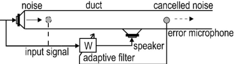
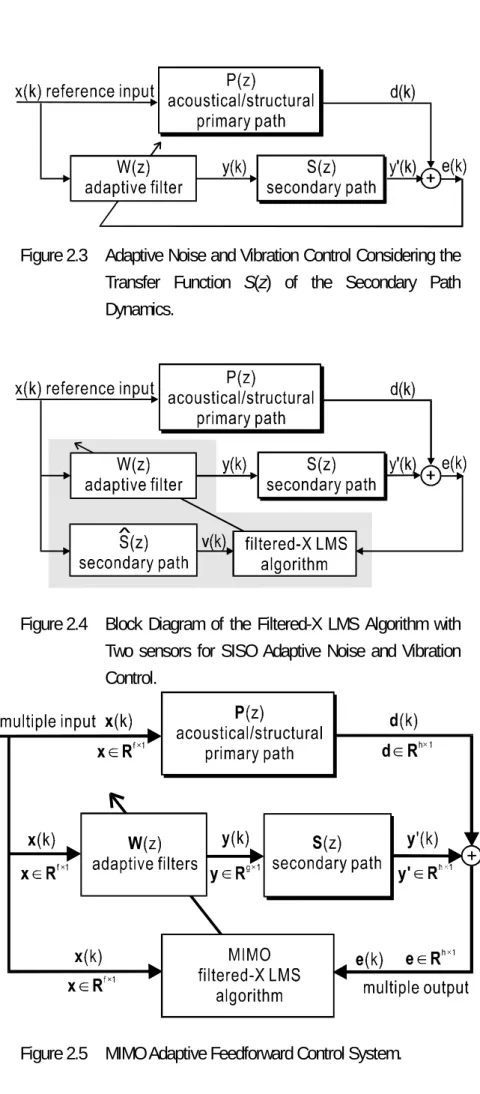
In noise and vibration control, it is not possible to get direct access to the adaptive filter output y(k) and the error signal e(k) because of the presence of acoustic devices and/or structural devices, generally called the secondary path devices.
In acoustical systems as shown in Fig. 2.1, the secondary path includes the actuator (speaker), the error microphone, and the acoustic field dynamics between the actuator and the error microphone. Similarly for structural vibration control as shown in Fig.
2.2, the secondary path in structural systems includes the low-pass filter, the power amplifier and the dynamics of the actuator and the error sensor. The control input from the adaptive filter can not be directly applied to system; it has to pass through the secondary path devices. Thus the adaptive noise and vibration control must be modified as shown in Fig. 2.3. The adaptive filter output has been processed by the secondary path dynamics of transfer function S(z) to yield the output y′(k). Thus, the LMS algorithm must be modified into the filtered-X LMS algorithm, since the output of the adaptive filter is filtered before entering the LMS algorithm.
The filtered-X LMS algorithm can be used only for the FIR adaptive filter.
The z-transform of the error signal e(k) can be found as
) ( ) ( ) (
) ( ) ( ) ( ) ( ) (
z W z V z D
z X z W z S z D z E
+
=
+
= (2.1)
where X z( ), D z( ), S(z), and W(z) are the z-transforms of the reference input x(k), the desired output d(k), the secondary path transfer function, and the adaptive filter, respectively, and V(z)=S(z)X(z). The error signal e(k) can be rewritten as
) ( ) ( ) ( )
(k d k k k
e = +ϕT θ (2.2)
where ϕ(k)=[v(k)v(k−1)Lv(k−n)]T, v(k) is the inverse z-transform of V z( ),
T
bn
b b
k) [ ]
( = 0 1L
θ .
The filtered-X LMS algorithm as shown in Fig. 2.4 has an update law similar to that in LMS algorithm (Burgess, 1981),
) ( ) ( ) ( ) 1
(k θ k e k ϕ k
θ + = −µ . (2.3)
In a multi-input and multi-output (MIMO) adaptive control system with f reference sensors, g actuators, and h error sensors, the block diagram of the multiple-reference-multiple-output system using the filtered-X LMS algorithm is shown in Fig. 2.5. The controller is in an adaptive FIR filter matrix W(z) of dimension g× f , with f reference input xi(k), i=1,2,..., f and g secondary path output )yj(k , j=1,2,...,g . S(z) represents the secondary path dynamics of dimension h×g.
The output of the MIMO adaptive filter can be presented by
=
) (
) (
) (
) ( )
( )
(
) ( )
( ) (
) ( )
( ) (
) (
) (
) (
2 1
2 1
2 22
21
1 12
11
2 1
z x
z x
z x
z W z
W z W
z W z
W z W
z W z
W z W
z y
z y
z y
f gf
g g
f f
g
M L
M M M M
L L
M . (2.4)
By taking the inverse z-transform, the jth filter output is
) ( ]
) ( [
)
(k 1( 1) k 1( ) k
yj = 0× j− ⋅f⋅n xT 0×g−j⋅f⋅n w , (2.5) where n is the dimension of each FIR adaptive filter. The generalized f ⋅n×1
input vector is
T
f k n
x k
x k x n k x k
x k x
k) [ ( ) ( 1) ( 1) ( ) ( 1) ( 1)]
( ≡ 1 1 − L 1 − + 2 2 − L − +
x (2.6)
and the generalized g⋅ f ⋅n×1 weight vector is
T n gf
n w w w
w w
w
k) [ ] ( ≡ 11,0 11,1 L 11, −1 12,0 12,1 L ,−1
w , (2.7)
where the subscripts j, i, and l in wji,l each denotes the jth filter output, the ith filter
input, and the lth weight of the inverse z-transform of Wji(z), respectively. The
filter output can be rewritten in a vector form as ) ( ) ( )
(k T k w k
y =X , (2.8)
where
T
g k m
y k
y k y m k y k
y k y
k) [ ( ) ( 1) ( 1) ( ) ( 1) ( 1)]
( ≡ 1 1 − L 1 − + 2 2 − L − +
y (2.9)
≡
) ( ' )
( ' ) ( ' ) (
k k
k k
x 0 0
0 0
0 x
0
0 0
x X
L O M
L L
(2.10)
)]x'(k)≡[x(k) x(k−1) L x(k−m+1 , (2.11)
Matrix X(k) is of dimension (g⋅ f ⋅n)×(g⋅m) and m is the dimension of each secondary path transfer function Spj(z) in S(z). The weight matrix S(k) of dimension )h×(g⋅m and the weight vector of the secondary path transfer function
)
pj(k
s can be written as
=
) ( )
( ) (
) ( )
( ) (
) ( )
( ) ( )
(
2 1
2 22
21
1 12
11
k k
k
k k
k
k k
k k
hg h
h
g g
s s
s
s s
s
s s
s
L M M M M
L L
S (2.12)
)]spj(k)≡[spj,0(k) spj,1(k) L spj,m−1(k . (2.13) The MIMO filtered-X LMS algorithm can be derived in a procedure. The
generalized error signal vector is
), ( ) ( ) ( ) (
) ( ) ( ) (
) ( ) ( ) (
k k k k
k k k
k k
k
T w
d
y d
y d
e
X S S +
=
+
=
′ +
=
(2.14)
where )d(k is the generalized desired signal vector,
T
h k m
d
m k d k
d k d m k d k
d k d k
)]
1 (
) 1 (
) 1 ( ) ( ) 1 (
) 1 ( ) ( [ )
( 1 1 1 2 2 1
+
−
+
−
− +
−
−
≡
L
L L
d (2.15)
The cost function of the adaptive filter is defined as the sum of the mean-square errors
)}ξ =E{eT(k)e(k . (2.16)
However, this error criterion is generally not practical. Instead, assuming that each mean-square error is stochastic and can be approximated by its instantaneous square error, Eq. (2.16) is approximated as
) ( ) ( )
ˆ(k =eT k e k
ξ . (2.17)
The square error is minimized by the steepest decent method, ) ˆ( ) 2
( ) 1
(k + =w k − µ∇ξ k
w (2.18)
).
( ) (
) ( ) ( ) ( ) ˆ(
k k
k k k
k T
e e X
S X
≡ ′ ξ =
∇ (2.19)
The generalized MIMO filtered-X LMS algorithm can be obtained ) ( ) ( )
( ) 1
(k w k k e k
w + = −µX′ . (2.20)
where X′( )k is the (g⋅ f ⋅n)×h matrix of the filtered reference signal.
2.2 Feedback Controller in Feedforward Algorithm
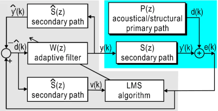
Adaptive noise and vibration control in two-sensor configuration as shown in Fig 2.4 requires two sensors: one reference sensor in the upstream to measure the reference input x(k) and another error sensor in the downstream to measure the error signal e(k). For noise systems with spatially incoherent noise induced by turbulence or during propagation paths, it is difficult, if not impossible, to measure the reference signal. Similarly for vibration systems, to measure the pure reference signal is difficult. An effective controller design is to use only the error sensor and its measurement to synthesize the reference signal. The concept is similar to a feedback system implemented by an adaptive feedforward controller. Careful examination indicates that the adaptive noise and vibration cancellation system by using only an error sensor is implementable. Figure 2.6 depicts the block diagram of the adaptive feedback control by FIR adaptive filter in single sensor configuration,
where e(k) is the error sensor output and y(k) is the control input to the actuator (secondary path). The error sensor measures the sum of the primary path noise or vibration signal d(k) and the secondary path canceling output y′(k). The objective is to generate y(k) based on the measurement of e(k) so as to minimize the energy of vibration or acoustical noise.
If the transfer function of the secondary path dynamics S(z) is known or can be estimated by system identification, then an estimation of the (uncanceled) primary path signal d(k) at the sensor location can be obtained by subtracting the reflected component of the actuator output from the sensor measurement e(k), since y(k) is known exactly. dˆ k( ) can then be filtered by the FIR adaptive filter to yield the input of actuator y(k). The weight vector of the FIR adaptive filter are updated by the filtered-X LMS algorithm based on the error signal e(k) such that the energy of the canceled noise is minimized. Because most systems are of non-minimum phase due to the time delay from the secondary path dynamics, the transfer function S(z) will then have zeros located outside of the unit circle such that the system is prone to instability. For this reason, FIR adaptive filter is preferable over IIR filter in adaptive noise and vibration control in the sense of system stability.
For the adaptive feedback noise and vibration control system shown in Fig. 2.6, the error signal can be written as
) ˆ( ) ( ) ( ) ( )
(z D z S zW z D z
E = + , (2.21)
where )E(z , )D(z and Dˆ z( ) are the z-transforms of e(k), )d(k and dˆ k( ), respectively. An estimation of the primary path signal d(k) can be obtained by
) ˆ( ) ( ) ˆ( ) ( )
ˆ(z E z S z W z D z
D = − . (2.22)
Equation (2.46) can be rearranged as
) ( ) ˆ( 1
) ) (
ˆ(
z W z S
z z E
D = +
. (2.23)
Substituting Eq. (2.23) into Eq. (2.21),
) ( ) ˆ( 1
) ( ) ( ) ) ( ( ) (
z W z S
z E z W z z S D z
E = + +
, (2.24)
one can find the overall transfer function H(z) of the feedback system from d(k) to )e(k
) ( )) ( ) ˆ( ( 1
) ( ) ˆ( 1 )
( ) ) (
( S z S z W z
z W z S z
D z z E
H + −
= +
= . (2.25)
If )Sˆ(z)≠S(z , )H(z is an infinite impulse response system, i.e., e(k) can not be completely canceled. Therefore, system identification of the secondary path dynamics is critical to the performance of the feedback system.
Suppose Sˆ(z)=S(z) and the secondary path dynamics has c time delay
samples, i.e., Sˆ(z)=z−cSˆ′(z), where Sˆ z′( ) has no delay, one may find the overall transfer function
) ( ) ˆ( ) 1
( )
( z S z W z
z D
z
E = + −c ′ . (2.26)
If E(z)/D(z) is close to zero, i.e., e(k) converges to zero, W(z) will be a noncausal filter,
) ˆ( )
( S z
z z W
c
− ′
→ . (2.27)
Thus, the adaptive feedback control system shown in Fig. 2.6 is prone to nonstationary noise and vibration control. Only periodic signals can be completely canceled because of the effect of the time delay. The performance of the control system is sensitive to the time delay c and the sensor/actuator dynamics Sˆ z′( ). However, the controller design is still effective in stationary periodic disturbance cancellation. The position of the sensor and actuator, whether in feedback or
feedforward configuration, are also critical to the system performance of active noise control. For stable maximum attenuation, the error sensor is required to be placed very close to the actuator in order to minimize the time delay c. Such requirement was seen in many of the previous active noise control studies.
In order to implement the adaptive noise and vibration control system as described above, one first needs to identify the secondary path dynamics S(z).
System identification of the secondary path dynamics is introduced in the next section.
2.3 ARX System Identification Model
A dynamic system can be conceptually described as in Fig. 2.7. The system is driven by input variable u t( ) and disturbance n(t). In many signal processing applications the input may not be known apriori. System identification is performed by using some sort of input signal such as step, sinusoid or random signal and observing the system’s input and output over a time interval. One then tries to fit a parametric model of the process by using the input and output sequences.
A commonly used parametric model is the ARX (controlled autoregressive) model
) ) ( ( ) 1 ) ( (
) ) (
( 1 1
1
q k k A q u
A q q B k
y = −l −− + − ε (2.28)
where A(⋅) and B(⋅) are polynomials in the delay operator q−1 A q( −1)= +a q1 − + +a qm −m
1 1 L (2.29)
B q( −1)= +b1 b q2 −1+ L +b qn − +n 1. (2.30) l is the number of delays from input to output, and m and n are the orders of the
respective polynomials. The ARX model can be written by ) ( ) ( ) ( ) ( )
(q 1 y k B q 1 u k l k
A − = − − +ε (2.31)
or explicitly
) ( ) 1 (
) 1 (
) (
) ( )
1 ( ) (
2 1
1
k n
l k u b l
k u b l k u b
m k y a k
y a k y
n m
ε + +
−
− +
+
−
− +
−
=
− +
+
− +
L
L (2.32)
or y(k)=φT(k)θ +ε(k) (2.33)
where
n T
l k u l k u m k y k
y
k) [ ( 1) ( ) ( ) ( 1)]
( = − − L− − − L − − +
φ (2.34)
T n
mb b
a
a ]
[ 1L 1L
θ = (2.35)
The next step is to estimate the unknown parameter θ by the least square (LS) method. The task is to compute the model output yˆ k( ), yˆ(k)=φT(k)θˆ, from the parameter θˆ such that the model output agrees as closely as possible with the measured output y(k) in the sense of least square. Define the error equation of the identification as
θ φ ( )ˆ )
( ) ( ˆ ) ( )
(k = y k −y k = y k − T k
ε (2.36)
The least square error is
( )
( )2 ˆ 1 ) ( ) 2 (
) 1 2 (
) 1 , (
1
2
1
2 y i i k k
i k
L T
k
i
T k
i
ε ε θ
φ
θ =
∑
=∑
− = ( )=
=
ε (2.37)
where
θ
ε = y−yˆ= y−Φ ˆ (2.38)
k T
y y
y
k) [ (1) (2) ( )]
( = L
y (2.39)
k T
k) [ (1) (2) ( )]
( = ε ε L ε
ε (2.40)
k T
k 1) [ (0) (1) ( 1)]
( − = φ φ L φ −
Φ (2.41)
Equation (2.61) can be rewritten by