Generalized method for three-dimensional slope stability analysis

Generalized Method for Three-Dimensional Slope Stability

Analysis

Ching-Chuan Huang

; Cheng-Chen Tsai

; and Yu-Hong Chen

Abstract: This paper describes an extension of a new three-dimensional共3D兲 stability analysis method, including formulation, com-parative studies, and examples of new application. The new method uses ‘‘two-directional force and moment equilibrium’’ in the stability analysis of 3D potential failure mass with arbitrary shapes. The use of this new method has resulted in a novel situation wherein the direction of the resultant shear force共or direction of sliding兲 generated on the potential failure surface can now be calculated instead of the guesswork assumptions that were formerly made. It is also demonstrated that this new method eliminates the labor-intensive work for establishing local coordinate systems performed in conventional 3D analysis. Consequently, this new method facilitates a computer-aided 3D search for the critical failure surfaces in slope areas.

DOI: 10.1061/共ASCE兲1090-0241共2002兲128:10共836兲

CE Database keywords: Slope stability; Three-dimensional analysis; Sliding.

Introduction

Three-dimensional 共3D兲 slope stability analysis methods, based on limit equilibrium or variational calculus, have been proposed by various researchers since the 1970s. A majority of these meth-ods assumed a symmetrical plane for the failure mass in order to eliminate the static indeterminate condition 共Baligh and Azzouz 1975; Hovland 1977; Chen and Chameau 1982; Leshchinsky et al. 1985; Xing 1988; Leshchinsky and Huang 1992b兲. In some of the remaining methods共e.g., those of Ugai 1985; Hungr 1987; Lam and Fredlund 1993兲 a symmetrical plane is not assumed in the limit equilibrium formulation. However, these methods re-tained the characteristics of 3D symmetrical analysis because force and/or moment equilibrium were excluded in the direction transverse to the sliding. As pointed out by Hungr et al.共1989兲, the unbalanced force in the transverse direction of sliding may account for the errors in the calculated value of safety factors for a sliding wedge. The effect of 3D slope geometry on the slope stability has been studied by Xing共1987兲 on concave slopes, and also by Leshchinsky and Mullett 共1987兲 on conical deposits formed by homogeneous soils. These studies focused on the effect of 3D symmetrical slope geometry on the safety factors of the slopes. To date, 3D stability analysis was used mainly in ‘‘back-analysis’’ of the failure for a known failure surface. Searching for 3D potential failure surfaces for filled and/or natural slopes has

never been done successfully except on planar surfaces. Two major disadvantages inherent in all of the foregoing 3D slope stability analysis methods are

1. Work involved in guessing a plane of symmetry, because in areas of irregular geometrical and/or geological conditions, the direction of potential sliding may vary considerably and may also be difficult to ‘‘guess’’ in advance.

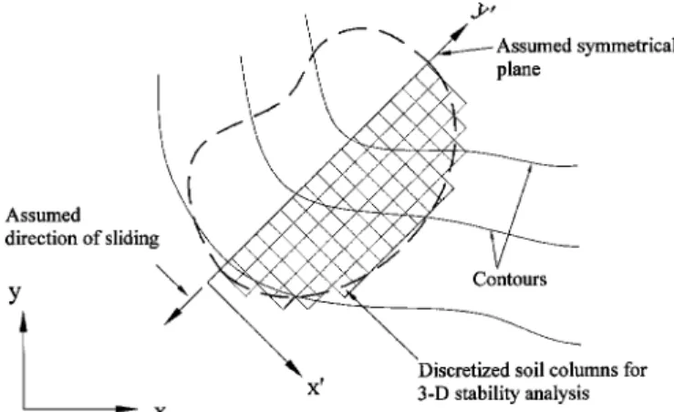
2. Work involved in establishing local coordinate system for various potential failure surfaces, i.e., when using these methods, a local coordinate system must be established so that the y⬘共or x⬘兲 axis is identical to the assumed direction of sliding共see Fig. 1兲.

The above disadvantages come from the traditional ‘‘one-directional moment 共or force兲 equilibrium’’ used in these limit equilibrium methods. That is, the moment共or force兲 equilibrium is only satisfied in an ‘‘assumed’’ direction of sliding共i.e., the y⬘ direction as seen in Fig. 1兲. It has been shown by Huang and Tsai 共2000兲 that the use of ‘‘two-directional moment equilibrium’’ in a rotational slip surface may eliminate the above disadvantages.

1_{Professor, Dept. of Civil Engineering, National Cheng Kung Univ.,}

Tainan 70101, Taiwan. E-mail: samhcc@mail.ncku.edu.tw

2_{Engineer, RAITO Engineering Corp., Kuan Chien Rd., 9th floor,}

Taipei, Taiwan; formerly, Graduate Student, Dept. of Civil Engineering, National Cheng Kung Univ., No. 1, Ta-Hseih Rd., Tainan, Taiwan.

3_{Graduate Student, Dept. of Civil Engineering, National Cheng Kung}

Univ., No. 1, Ta-Hseih Rd., Tainan, Taiwan.

Note. Discussion open until March 1, 2003. Separate discussions must be submitted for individual papers. To extend the closing date by one month, a written request must be filed with the ASCE Managing Editor. The manuscript for this paper was submitted for review and possible publication on June 1, 2001; approved on February 27, 2002. This paper is part of the Journal of Geotechnical and Geoenvironmental

Engineer-ing, Vol. 128, No. 10, October 1, 2002. ©ASCE, ISSN 1090-0241/2002/

10-836 – 848/$8.00⫹$.50 per page.

Fig. 1. Schematic of coordinate transformation and assumptions

Based on this new concept, the x or y axis is not rotated to con-form to an assumed direction of sliding 共or a direction of the symmetrical plane兲, and the direction of potential sliding can be ‘‘calculated’’ rather than assumed in the analysis. In the study by Huang and Tsai 共2000兲, the concept of two-directional 共2D兲 mo-ment equilibrium was verified when based on the analyses of rotational failure mechanisms. To facilitate the practical use of the new concept proposed by Huang and Tsai 共2000兲, two problems must be solved: 共1兲 the applicability of the new concept to non-rotational failure mechanisms, and 共2兲 the validity of limit equi-librium formulations in a unified 3D coordinate system. Because of the above, a generalized 3D slope stability analysis method based on two-directional moment and force equilibrium and its

computer algorithm were developed. The basic formulations and assumptions regarding the force and moment equilibrium were extended from the 2D slice method suggested by Janbu共1973兲.

Formulation

A potential sliding mass was divided into a group of square soil columns共Fig. 2兲. For a column 共i, j兲, the following notations are used:

⌬␰x_{i, j}⫽␰x_i⫺1,j⫺␰x_{i, j} (1) ⌬␰y_{i, j}⫽␰y_{i, j⫺1}⫺␰y_{i, j} (2) The notation␰ in the above equations represents the intercol-umn normal force E, vertical shear force X, and horizontal shear force H, as shown in Fig. 3. When the force equilibrium is in the vertical direction for column共i, j兲, and the sign convention for the force is positive when acting toward a positive x, y, or z direction, then Ni, j⫽ ⫺共Wi, j⫹Pv_{i, j}兲⫺⌬Xx_{i, j}⫺⌬Xy_{i, j}⫺Si, jf3_{i, j} g3_{i, j} (3) in which Ni, j⫽Ni, j⬘ ⫹Ui, j (4) Ni, j,Ni, j⬘⫽total and effective normal force acting on the column

base, respectively; Ui, j(⫽ui, j•Ai, j)⫽uplifting force normal to the

failure surface; ui, j⫽pore water pressure; Ai, j⫽area of column

base;Wi, j⫽self-weight of soil column 共positive for upward force兲;

Pv_{i, j}⫽vertical load on top of the column; Si j⫽mobilized shear

Fig. 2. Planar view of divided columns

Fig. 3. Three-dimensional view of forces acting on soil column

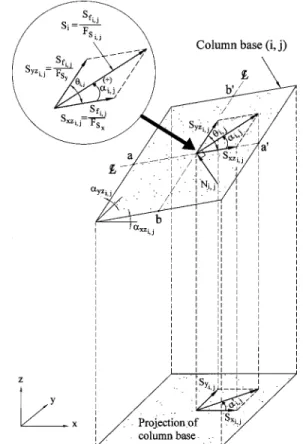
Fig. 4. Components of force acting on column base and their

resistance of soil on column base; and g3_{i, j}, f3_{i, j}⫽z components of the unit vectors for Ni, j,Si, j 关see Eqs. 共29兲 and 共31兲 in the

Appendix兴.

The safety factor on the column base, FS_{i, j}, is expressed as

FS_{i, j}⫽ Sf_{i, j} Si, j ⫽关Ci, j⫹共Ni, j⫺Ui, j兲tan␾i, j兴 Si, j (5) where Sf_{i, j}⫽ultimate shear strength of soil on the column base 共i,

j兲 based on Mohr–Coulomb’s failure criterion; Ci, j⫽cohesive

strength component 共⫽ci, j•Ai, j,ci, j⫽cohesion intercept, Ai, j

⫽area of column base兲; and ␾i, j⫽friction angle on the column

base.

Based on the law of sines and the force polygon shown in Fig. 4, in which,␣i, jrepresents a positive angle between Si, j and the

line a – a⬘, which is formed by the intersection between the x – z plane and the bottom plane of soil column, the following equa-tions are obtained:

FS_y FS_x⫽ sin共␪i, j⫺␣i, j兲 sin␣i, j , 0⬍␣i, j⬍␪i, j (6) FS_{i, j}⫽ FS_xsin共␪i, j⫺␣i, j兲 sin␪i, j , 0⭐␣i, j⬍␪i, j (7) FS_{i, j}⫽ FS_ysin␣i, j sin␪i, j , 0⬍␣i, j⭐␪i, j (8)

in which,␪i, j⫽angle between a – a⬘and b – b⬘共Fig. 4兲. The value

of␪i, j is always positive and is derived in the Appendix. For the

␣i, j⫽0° condition, Eq. 共7兲 is reduced to FS_{i, j}⫽FS_x. This

repre-sents a sliding towards the ⫹x or ⫺x direction. For the ␣i, j

⫽␪i, jcondition, Eq.共8兲 is reduced to FS_{i, j}⫽FS_y, implying

poten-tial sliding towards the ⫹y or ⫺y direction. In these special cases, the local safety factors FS_{i, j} for all columns are identical

and are equal to FS_xor FS_y. This shows that the safety factor used

in the present study is an extension of the safety factor used in conventional 2D and 3D stability analysis. Substitute Eq.共7兲 into Eq.共5兲, then Si, j⫽ 关Ci, j⫹共Ni, j⫺Ui, j兲tan␾i, j兴 FS_x sin␪i, j sin共␪i, j⫺␣i, j兲 (9) By substituting Eq. 共3兲 into the above equation, the mobilized shear force, Si, j, can be expressed as

Si, j⫽

再

冉

冊

冎

冉

冊

⌬Ex_{i, j}⫹⌬Hy_{i, j}⫹Ni, jg1_{i, j}⫹Qx_{i, j}⫹Si, jf1_{i, j}⫽0 (11) in which, ⌬Ex_{i, j}⫽Ex_{i, j⫺1}⫺Ex_{i, j}. It should be noted that ⌬Hy_{i, j}

(⫽Hy_{i, j⫺1}⫺Hy_{i, j}) may induce ‘‘torque’’ along the z axis. The

disturbance force induced by the torque along the z axis of the failure mass was assumed to be minor in the present study. There-fore, ⌬Hy_{i, j}⫽0 was used in the following analyses. The authors

believe that the values⌬Hy_{i, j}and⌬Hx_{i, j}(⫽Hx_i⫺1,j⫺Hx_{i, j}) can be

calculated by incorporating the equation of torque equilibrium for each soil column, the boundary conditions, and the intercolumn force functions for Hx_{i, j} and Hy_{i, j} similar to those proposed by

Mogenstern and Price共1965兲.

Rearranging Eq. 共11兲 and substituting Ni, j with Eq.共3兲, then

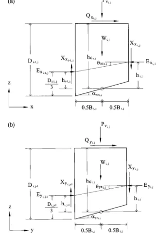
Fig. 5. 共a兲 Projection of intercolumn force on x – z plane. 共b兲

Projec-tion of intercolumn force on y – z plane.

⌬Ex_{i, j}⫽ 共Wi, j⫺Pv_{i, j}兲⫹⌬Xx_{i, j}⫹⌬Xy_{i, j} g3_{i, j} g1_{i, j} ⫹Si, j

冉

冊

冉

冊

Sf_{i, j} in the above equation was defined in Eq. 共5兲. It can be

ob-tained by using Eqs.共3兲, 共5兲, and 共10兲.

The sum of⌬Ex_{i, j}for a whole sliding mass can be expressed

as

兺

兺

兺

兺

兺

兺

can be expressed as FS_x⫽ ⫺兺j⫽1 m _兺 i⫽1 n A1 兺j⫽1 m _兺 i⫽1 n _B1⫺兺 j⫽1 m _共E x_{o, j}⫺Ex_{n, j}兲 (15) in which Ex_{o, j} and Ex_{n, j} denote the horizontal thrusts applied at

two ends of the j th row of the soil column共see Fig. 2兲. Substitute Eq.共8兲 into Eq. 共5兲, then the shear force, Si, j, can be expressed as

a function of FS_y Si, j⫽ Sf_{i, j} FS_{i, j}⫽ 关Ci, j⫹共Ni, j⫺Ui, j兲tan␾i, j兴 FS_y sin␪i, j sin␣i, j (16) in which FS_y⫽safety factors against sliding along the y direction.

Substitute Ni, j in the above equation with Eq. 共3兲, where the

mobilized shear force Si, jcan be expressed as

Si, j⫽

冋

冉

冊

册

冉

冊

⌬Ey_{i, j}⫽⫺Ni, jg2_{i, j}⫺Qy_{i, j}⫺Si, jf2_{i, j} (18) By substituting Eq.共3兲 into Eq. 共18兲, ⌬Ey_{i, j}can be expressed as

⌬Ey_{i, j}⫽ 共Wi, j⫹P␯i, j兲⫹⌬Xxi, j⫹⌬Xyi, j g3_{i, j} g2_{i, j} ⫹Si, j

冉

冊

Substitute Eq.共19兲 with Eq. 共16兲, then it can be expressed as ⌬Ey_{i, j}⫽ A2 FS_y⫹B2 (20) A2⫽Sf_{i, j} sin␪i, j sin␣i, j

冉

冊

Sf_{i, j} in the above equation was defined in Eq. 共5兲. It can be

ob-tained by using Eqs. 共3兲, 共5兲, and 共17兲. By summation of ⌬Ey_{i, j}

for a whole sliding mass and by introducing the boundary force, the safety factor FS_ycan be expressed as

FS_y⫽ ⫺兺in⫽1兺jm⫽1A2 兺i⫽1 n _兺 j⫽1 m _B2⫺兺 i⫽1 n _共E

y_o,i⫺Ey_m,i兲

(21) in which Ey_o,i and Ey_m,i denote the horizontal thrusts applied at

two ends of the ith row of the soil columns 共see Fig. 2兲. The safety factor for the whole sliding mass, FS, is defined as

FS⫽ 兺j⫽1 m _兺 i⫽1 n _S f_{i, j} 兺j⫽1 m _兺 i⫽1 n _S i, j (22) In this equation, the values of Sf_{i, j} are obtained by using a

method similar to that for Eq.共13兲 or 共20兲, and the values of Si, j

are obtained by using Eq.共10兲 or 共17兲. It is noted that the use of a constant value of safety factor, FS⫽Sf_i/Si, in conventional 2D

and 3D slope stability analyses, is identical to the use of FS

de-fined in Eq. 共22兲.

The normal force on the lateral face of column Ex_{i, j} was

as-sumed to apply at 1/3 the height of the side face of the column

Fig. 8. Two-dimensional failure surface reported by Fredlund and

Krahn共1977兲

Fig. 9.Center section of circular three-dimensional failure surface in

cohesive slope

Table 1. Safety Factors for Two-Dimensional Failure Surfaces Case number

Fredlund and Krahn

共1997兲

Morgenstern and Price

共1965兲a

Leshchinsky and Huang

共1992b兲

Rigorous method in the present studyb

1 2.076 –2.083 2.085 2.080 2.066共2.034–2.066兲c

2 1.764 –1.779 1.770–1.772 1.765 1.757共1.721–1.757兲c

3 1.364 –1.378 1.386 –1.394 1.312 1.387共1.382–1.405兲c

4 1.113–1.124 1.117–1.137 1.067 1.113共1.111–1.137兲c

Note: 共Description of slope and failure surface: case 1: circular, H⫽12.2 m, ␾⬘⫽20°, c⬘⫽28.7 kPa, ␥⫽18.8 kN/m3_{; case 2: same as in case 1, but} ru⫽0.25; case 3: composite, with weak layer: ␾⬘⫽10°, c⬘⫽0; case 4: same as in case 2, but ru⫽0.25兲.

a_{Reported by Fredlund and Krahn共1977兲.} b_{Total slice number⫽35.}

c_{Range of F}

关Fig. 5共a兲兴. It was based on the moment equilibrium about the center of the column base in the x direction,

Xx_{i, j}⫽⫺ ⌬Xx_{i, j} 2 ⫺⌬Exi, j hi, j Bi, j ⫹Ex_{i, j}tan␪xz_{i, j}⫺Qx_{i, j} hc_{i, j} Bi, j (23) When the total number of columns is sufficiently large and the width of columns is small, then⌬Xx_{i, j}→0 and ⌬Ex_{i, j}→0, and Eq.

共23兲 can be simplified to

Xx_{i, j}⫽Ex_{i, j}tan␪xz_{i, j}⫺ Qx_{i, j}hc_{i, j}

Bi, j

(24) Based on the moment equilibrium about the center of the base in the y direction 关Fig. 5共b兲兴 for column 共i,j兲, i.e.,

Xy_{i, j}⫽⫺ ⌬Xy_{i, j} 2 ⫺⌬Eyi, j hi, j Bi, j⫹Eyj tan␪y z_{i, j}⫺Qy_{i, j} hc_{i, j} Bi, j (25) When Bi, j is small, then⌬Xy_{i, j}→0, ⌬Ey_{i, j}→0, and Eq. 共25兲 can

be simplified to

Xy_{i, j}⫽Ey_{i, j}tan␪y z_{i, j}⫺ Qy_{i, j}hc_{i, j}

Bi, j

(26) Eqs.共24兲 and 共26兲 are used in the present study for the rigorous analyses.

Analytical and Numerical Considerations

Fig. 6 shows the sign conventions for forces and angles used for calculating the safety factor for potential sliding in all possible

directions. For example,␣i, jrepresents a positive angle from the

positive or negative direction of the x axis. When the mobilized shear force, Si, j, is oriented within⫹x⬙and⫹y⬙directions

共cor-responding to a sliding within the⫺x⬙ and⫺y⬙ directions兲, the unit vectors ( f1_{i, j}, f2_{i, j}, f3_{i, j}) presented in the Appendix are appli-cable. For the mobilized shear force in any other direction, the signs of f1_{i, j} and f2_{i, j} must be changed accordingly. It is noted that the terms B1 and B2 in Eqs. 共13兲 and 共20兲, respectively, represents the sliding force on each column base. They are func-tions of the components of the unit vector (g1_{i, j},g2_{i, j},g3_{i, j}) which are determined by the inclination of the column base 共see the Appendix兲. Therefore, for a potential failure surface, its quadrant for the direction of sliding is determined by the signs of the sum of B1 共i.e.,兺兺B1兲 and B2 共i.e.,兺兺B2兲, which are expressed in Eqs.共15兲 and 共21兲, respectively. A scheme showing the relation-ships of the directions of Si, j, the signs of f1_{i, j}and f2_{i, j}, and the signs of 兺兺B1and兺兺B2is shown in Fig. 6. A problem may be encountered in the numerical procedure when the direction of sliding coincides with the x⬙or y⬙axis. As shown in Eq.共6兲: 1. When ␣i, j→␪i, j, then FS_x→⬁; this indicates sliding

to-wards the⫹y⬙ or⫺y⬙ direction;

2. When␣i, j→0, then FS_y→⬁; this indicates sliding towards

the⫹x⬙ or⫺x⬙direction.

A detection system was established to detect the above two conditions and to avoid possible numerical difficulties. The fol-lowing criterion was used first:

兺兺B1 兺兺B2⭓␧d or 兺兺B1 兺兺B2⭐ 1 ␧d (27)

Fig. 10. Calculated values of FSversus number of columns for circular failure surface in cohesive slope

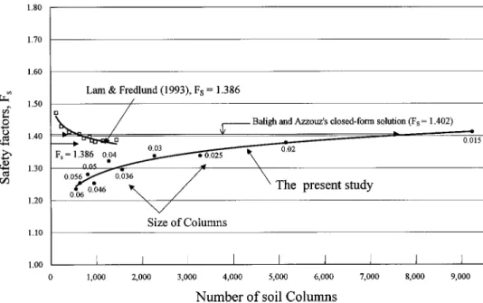
Table 2. Result of Comparative Study Using Three-Dimensional Failure Surfaces Reported by Baligh and Azzouz共1975兲 Baligh and Azzouz共1975兲

close-form solution Hungr共1987兲 Lam and Fredlund共1993兲 Simplified method in the present study

1.402 1.422 1.402共540兲 1.412共9,238兲a

— — 1.386共1,200兲 1.379共5,152兲a

A second criterion was then used in the subsequent calculations: FS_y FS_x⭓␧d or FS_y FS_x⭐ 1 ␧d (28) In the present study, ␧d⫽100 was tentatively suggested. Its

validity will be examined later. When one of the above conditions is fulfilled, the program switches into the one-directional equilib-rium calculations. That is, the problem was simplified into a sym-metrical one共with respect to the x or y axis兲. A personal computer program was established based on the above formulations. The computer algorithm for calculating a safety factor for a specific failure surface is shown in Fig. 7. For the sake of simplicity, only the flow chart for the case of␣i, j⫽0 and ␣i, j⫽␪i, j is shown. In

the computer program, Eq.共28兲 was checked whenever new FS_x

and F_S

y were generated. The present method simultaneously solves equilibrium equations for two independent directions.

Equations in either direction are analogous to those proposed by Janbu共1973兲 in a statically determinate 2D system, except for the following differences:

1. The horizontal shear force H_x

i, jand Hyi, jexist in the present 3D equilibrium system; and

2. An unknown parameter,␣_{i, j}, which represents the direction of resultant shear resistance on the column base, was intro-duced for each column.

The static indeterminate condition induced by 共1兲 was elimi-nated by assuming ⌬Hx_{i, j}⫽⌬Hy_{i, j}⫽0, as mentioned previously;

and共2兲 was solved by introducing Eq. 共6兲 for each column. Con-sequently, the 3D system presented herein is statically determi-nate.

Verification

The integrity of the calculation procedure was ensured by double checking the values of FS_{i, j}. For all cases presented in this paper,

FS_{i, j}for each column was calculated using Eq.共7兲 or 共8兲, and then

double checked by using Eq. 共5兲. The differences between the calculated values of FS_{i, j}using Eq.共7兲 or 共8兲 and those using Eq.

共5兲 were negligible. The validity of the method proposed in the present study has been further examined by using a 2D case共Fig. 8兲 reported by Fredlund and Krahn 共1977兲. A 2D failure surface may be deemed to be a special case in a generalized 3D one. In this case, the failure surface was simplified as a cylinder rotating about an axis parallel to the y axis 共i.e., ␣i, j⫽0 for every

col-umn兲, and by ignoring the resistance at both ends of the cylinder. The calculated values of FScorresponding to the slope described

in Fig. 8 are summarized in Table 1. It is seen that the rigorous method used in the present study rendered comparable results to other rigorous methods. Slightly different geometries were found among the 2D slope depicted by Fredlund and Krahn 共1977兲, Xing 共1987兲, Leshchinsky and Huang 共1992a兲, and Lam and Fredlund共1993兲. The calculated ranges of FSwere based on these

different geometries and are summarized in the parentheses in Table 1. It can be seen that the maximum error in FS, induced by

the errors in the geometry of the slope, was smaller than 2.3%.

Fig. 11. Three-dimensional failure surface reported by Hungr et al.

共1989兲

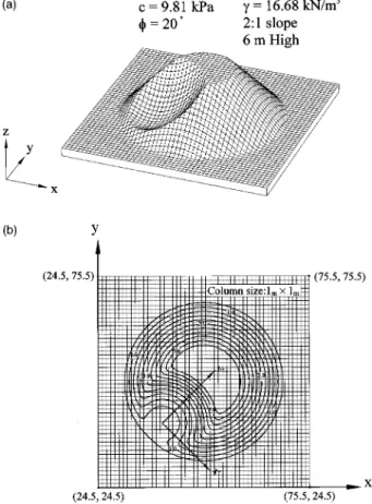
The proposed method was also compared with that reported by Baligh and Azzouz共1975兲. In this comparative study, a 3D, sym-metrical, circular failure surface in a cohesive slope, as shown in Fig. 9, was used, and the results are summarized in Table 2. When a sufficient number of soil columns was used共i.e., a total number of 9,238 columns with size of 0.015⫻0.015兲, the calculated value of FS, using the simplified method, differed from the close-form

solution within 0.7%. Detailed information on the FS versus the

number of soil columns relationships is shown in Fig. 10. These relationships, reported by Lam and Fredlund共1993兲, are also plot-ted. It is seen that the present study demonstrated a consistent trend in approaching the close-form solution when the numbers of soil columns were increased. The difference in the patterns of FS

versus the number of soil columns between the present study and that of Lam and Fredlund共1993兲 may come from different ways of discretization of the failure mass in soil columns. In the present study, the edges of the soil columns were kept inside the bound-ary of the failure mass. This resulted in conservative values of the integrated surface area of the failure mass in the calculation.

It is also noted that the rigorous method developed in the present study was not applied to the slope consisting of pure cohesive material as shown in Fig. 9. The difficulties associated with rigorous limit equilibrium method of slices, when analyzing a highly cohesive slope, have been discussed by Spencer 共1968, 1973兲 and by Ching and Fredlund 共1983兲. They suggested that a tension crack should be located at the top of the cohesive slope to avoid negative normal force on the slice base near the crest of the slope.

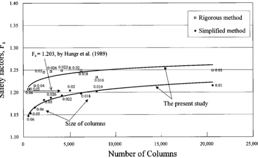
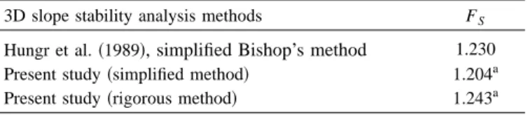
A comparative study was also conducted on a 3D circular surface in a c –␾ slope 共Fig. 11兲 reported by Hungr et al. 共1989兲. The results are summarized in Table 3. It is seen that the values of FS, obtained by using either simplified or rigorous approaches,

were comparable with those obtained by Hungr et al.共1989兲. It is also seen that the value of FS, obtained by using the rigorous

method, was about 3% larger than that in the simplified method. The FSversus the number of soil columns relationships is shown

in Fig. 12. The proposed methods gave a similar tendency to approach a steady value of FS when the number of soil columns

was increased.

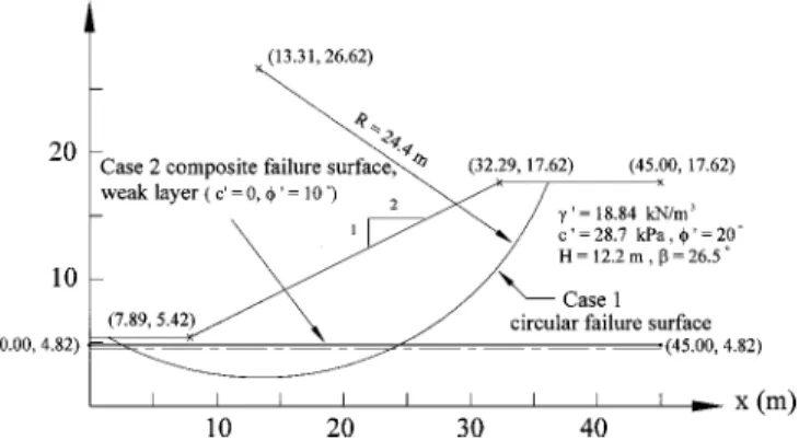
Table 4 summarizes the safety factor calculations on a com-posite failure surface共Fig. 13兲 that was directly extended from the

2D profile shown in Fig. 8. This failure surface was also used by Xing 共1987兲 and Lam and Fredlund 共1993兲. In the four cases investigated, the FS, obtained by using the proposed rigorous

method, were all slightly larger than the FSusing the simplified

one. In addition, the calculated FS, using the simplified method,

were reasonably close to the solutions generated in a simplified method proposed by Xing共1987兲. The results for case 3 obtained in the present study, using either simplified or rigorous methods, deviated from those obtained by Lam and Fredlund共1993兲 within 10%. The difference may be due to the following factors: 1. Different dimensions of the slope used in the analyses. As

mentioned by Sarma共1973兲 in a 2D analysis, errors induced from scaling a slope by various researchers may result in differences of FSas large as 18%;

2. Ranges of FS for all admissible solutions were not

consid-ered in either case;

3. Different assumptions on the intercolumn force; and 4. Different number of columns, and manner of assigning soil

columns. This was not reported by Lam and Fredlund 共1993兲.

Due to these possible factors, the 10% differences in the calcu-lated values of FSare considered tolerable. In four cases

investi-gated, the rigorous FSwere larger than the simplified ones within

a narrow range of 6.8 –7.1%. By comparing the values of rigorous FSshown in Tables 1 and 4, it was found that, for semi-spherical

failure surfaces, the increase in FS, due to the 3D effect, was

about 7.2– 8.5%, while for the composite failure surface with a weak layer, the increase in FS, due to the 3D effect, was 27–

Fig. 13. Three-dimensional composite failure surface used in

comparative study

Table 3. Results of Comparative Study Using Three-Dimensional

Failure Surfaces Reported by Hungr et al.共1989兲

3D slope stability analysis methods F_S

Hungr et al.共1989兲, simplified Bishop’s method 1.230

Present study共simplified method兲 1.204a

Present study共rigorous method兲 1.243a

a_{Total column number⫽5,080.}

Table 4. Results of a Comparative Study Using Three-Dimensional Failure Surfaces Case number Xing共1987兲

Lam and Fredlund共1993兲

共simplified method兲

Lam and Fredlund共1993兲

共rigorous method兲 共simplified method兲Present study a

Present study 共rigorous method兲a 1 2.122 — — 2.072 2.215 2 1.790 — — 1.781 1.908 3 1.548 1.558 1.603 1.645 1.757 4 1.278 — — 1.384 1.478

Note: 共Description of slope and failure surface: case 1: circular, H⫽12.2 m, ␾⬘⫽20°, c⬘⫽28.7 kPa, ␥⫽18.8 kN/m3_{; case 2: same as in case 1, but} ru⫽0.25; case 3: composite, with weak layer: ␾⬘⫽10°, c⬘⫽0; case 4: same as in case 2, but ru⫽0.25兲.

32%. The different 3D effects are attributable to the different influence of ‘‘end effects.’’ It is seen in Figs. 8 and 13 that, at a location away from the symmetrical plane, the failure surface consists of a stronger soil stratum (c⫽28.7 kPa,␾⫽20°). The above result infers the importance of using appropriate 3D slope stability analysis methods, especially for the case of weak-plane-induced 3D failure.

Applications

A truncated cone, deemed to be an ‘‘idealized hill,’’ was used to investigate the validity of calculating the direction of sliding共or the direction of the symmetrical plane兲 as well as calculating significant safety factor values for sliding masses which are asym-metrical to the x and/or y axes. A 3D and a planar view of this ‘‘hill’’ with a typical failure surface are shown in Figs. 14共a and b兲, respectively. The failure masses with identical geometry on the cone should possess identical safety factors (FS) against

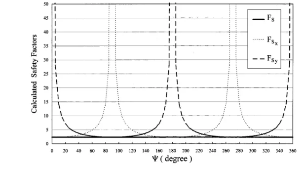
fail-ure. This was verified in this analysis. Parabolic functions were used to define the failure surface shown in Figs. 15共a and b兲. The parameters for the parabolic functions were selected arbitrarily. The results using the rigorous method, are shown in Fig. 16. It may be seen that both FS_x and FS_y showed periodical changes

with respect to the change in␺ 共␺⫽the angle between x axis and the projection of the symmetrical plane on the x – y plane, based on a counter-clockwise rotation关see Fig. 18共a兲兴. Meanwhile, val-ues of FS remained constant despite the changes in ␺. In this

analysis, the variation in FSwas within 2.348 –2.361 by using the

simplified method, and within 2.418 –2.467 by using the rigorous method. It is also seen that the value of FS_x or FS_y increases

dramatically when the value of ␺ approaches ‘‘singular’’ points 共i.e., ␺⫽0, 90, 180, and 270°兲. In this calculation, a pitch of ␺ 共i.e., ⌬␺兲 equal to 5° was used for all cases except when ␺ was close to the singular ones within⫾10°. In the latter cases, a small value of ⌬␺⫽0.1° was used to describe the curves accurately. Some typical cases are shown in Table 5. In this analysis, ␧d⯐100 in Eq. 共27兲 results in small values of ␣i, j 共smaller than

1°兲. This in turn resulted in very small difference in FS共involving

two directions of equilibrium兲 and FS_x共or FS_y, considering only

one direction of equilibrium兲 within only 1%. When the values of ␣i, j approach singular points the time needed for a converged

value of ␣i, j, according to Eq. 共6兲, is increased. In the present

study, the ‘‘secant method’’共see, e.g., Press et al. 1989兲 was used for solving Eq. 共6兲 to obtain an accurate value of ␣i, j for each

column. As an extreme case, Fig. 17 indicates that for a value of ␣i, japproximately equal to 0.1°, 10 repeat calculations were

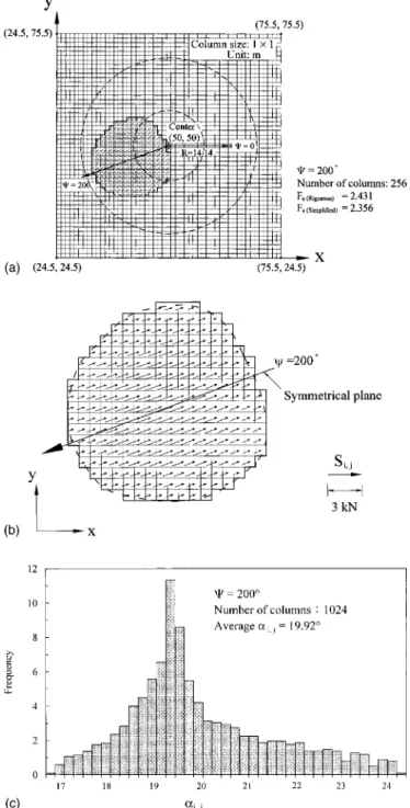
nec-essary. This indicated that the numerical procedure incorporated in the present study is capable of calculating accurate values of ␣i, j. Fig. 18共a兲 shows a planar view of a typical failure surface

with the calculated values of Si, j. An enlarged grid system and

the calculated values of Si, jare shown in Fig. 18共b兲. It should be

noted that the number of soil columns shown in Figs. 18共a and b兲 were purposely reduced to 256 for a clearer view whereas in the

Fig. 14. 共a兲 Three-dimensional view of ‘‘truncated cone’’ and failure

surfaces used in analysis;共b兲 planar view of truncated cone used in

analysis

Fig. 15. 共a兲 Longitudinal section of parabolic failure surface used in

analysis; 共b兲 transverse section of parabolic failure surface used in

analysis

Table 5. Relationships between Calculated Values of␣i, j⬘ and Total

Number of Columns

Total number of columns Average value of␣_{i, j}⬘

256 19.87°

1,024 19.92°

formal analyses, shown in Fig. 16 and Table 6, a total number of 1,024 columns were used. As expected, the calculated ‘‘directions of shear resistance’’ were approximately parallel to the plane of symmetry. This is further examined in a quantitative way by using the projected values of ␣i, j on the x – y plane共namely, ␣i, j⬘ 兲 as

shown in Fig. 18共c兲. It is seen that the average value of ␣i, j⬘ is

19.92°. The deviation between 19.92° and the theoretical value of 20° may come from the slightly less than symmetrical grid system used to simulate the failure mass. This was investigated by chang-ing the total number of columns in the analysis. The results are summarized in Table 5. It is seen that the mean values of ␣i, j

approach the ideal value of ␣i, j⫽20° when the number of

col-umns increases. Figs. 19共a and b兲 demonstrate the capability of calculating accurate intercolumn force. Two cases 共␺⫽180.1° and 270.1°兲 were selected because both cases are close to the singular ones, and are challenging in obtaining converged results.

It is seen that this method calculates identical values of intercol-umn force for corresponding colintercol-umns in these two sliding masses. It is also seen in Fig. 19共a兲 that negative normal force 共Ex_{i, j}and

Ey_{i, j}兲 exists near the crest of the failure mass. This may infer that

a tension crack is necessary. However, a discussion of this issue is beyond the scope of the present study.

It is seen from the results in Figs. 16 and 18共a兲 that most of the failure surfaces analyzed were asymmetrical to either the x or y axis共except those with ␺⫽0°, 90°, 180°, and 270°兲. Therefore, this calculation indirectly demonstrates that the new methods pro-posed herein are applicable to the stability analysis for asym-metrical 3D failure surfaces.

The generalized method proposed herein may promote the use of a slope stability program as an analytical tool to search for the sliding potential of a slope. To achieve this, in addition to the

Fig. 16. Calculated FS, FS_x, and FS_y for various directions of sliding

correct force and moment equilibrium formulations, the following three requirements should be met:

1. The use of appropriate shapes of failure surfaces, e.g., quad-rilateral, log spiral, or planar surfaces;

2. The use of efficient methods of optimization; and

3. A provision for sufficient geological and geometrical infor-mation.

These topics require more study in the future. For example, the use of the 3D potential failure surface optimization technique, as proposed by Yamagami and Jiang共1997兲, may substantiate topics 1 and 2 above. A limitation associated with the present method is when the side surface of the sliding mass is vertical. In this case,

the shear resistance, parallel to the direction of slide, along the side of the sliding mass is not taken into account in the present method. Therefore, an error in the calculated value of the 3D safety factor of the slope may occur to some extent depending on the geometry of the sliding mass and the inclination of the sliding plane 共Stark and Eid 1998兲. However, as mentioned before, this problem can be solved by incorporating a torque equilibrium equation for each soil column, the boundary force condition, and intercolumn force functions in the present method. In the case of an inclined 共or nonvertical兲 side surface of the sliding mass, the side surface can be regarded as part of the failure surface, and the present method is applicable.

Conclusions

A new 3D slope stability analysis method proposed by Huang and Tsai 共2000兲 is extended for sophisticated and computer-oriented 3D slope stability analysis. The new method introduces a force and moment limit equilibrium in two orthogonal directions to analyze the stability of a potential failure mass. As a result, the direction of sliding 共or the resultant shear force on the slip sur-face兲 is a part of the analytical solution rather than an assumption. Possible errors associated with assuming a symmetrical plane for a sliding mass are eliminated. This method was validated using 2D and 3D failure surfaces reported in the literature. A stability calculation on a truncated cone, which is deemed to be an ideal-ized hill, demonstrated the potential this method has for a com-puterized analysis to obtain a potential failure mass with an arbi-trary shape in a unified 3D coordinate system.

Acknowledgment

The present study was financially supported by the National Sci-ence Council, Taiwan, under Contract No. NSC 90-2211-E-006-011.

Fig. 18. 共a兲 Planar view of grids and failure mass sliding toward ␺

⫽200°; 共b兲 Enlarged view of calculated direction and intensities of

resisting shear force; and 共c兲 Distribution of ␣i, j⬘ for failure mass

under␺⫽200°

Table 6. Calculated Safety Factors for Masses Sliding Toward Various Directions

⌿ Simplified method Rigorous method

Number of columns 200° 共Quadrant I兲 FS⫽2.352 FS⫽2.436 1,024 FS_x⫽2.512 FS_x⫽2.602 FS_y⫽7.133 FS_y⫽7.376 225° 共Quadrant I兲 FS⫽2.361 FS⫽2.445 1,031 FS_x⫽3.402 FS_x⫽3.528 FS_y⫽3.402 FS_y⫽3.512 315° 共Quadrant II兲 F_S⫽2.361 F_S⫽2.440 1,031 F_S x⫽3.402 FSx⫽3.532 FS_y⫽3.402 FS_y⫽3.493 45° 共Quadrant III兲 FS⫽2.361 FS⫽2.471 1,031 FS_x⫽3.402 FS_x⫽3.557 FS_y⫽3.402 FS_y⫽3.557 135° 共Quadrant IV兲 FS⫽2.361 FS⫽2.460 1,031 FS_x⫽3.402 FS_x⫽3.519 F_S y⫽3.402 FSy⫽3.564

Fig. 19. 共a兲 Intercolumn force Xx_{i, j} and Xy_{i, j}in longitudinal direction共b兲 Intercolumn force Ex_{i, j}and Ey_{i, j}in transverse direction

Appendix

See Huang and Tsai共2000兲 for a complete derivation of the fol-lowing equations. The unit vector n normal to the column base may be expressed as共Fig. 20兲:

n⫽

再

冎

冑

The angle ␪ between Sxz and Syz on the column base may be

expressed as

␪⫽cos⫺1_共sin␣

xzsin␣y z兲 (30) The unit vector S, which represents the mobilized shear force on the column base, may be expressed as

S⫽

再

sin␪ ,

sin␣ cos ␣y z sin␪ , sin共␪⫺␣兲sin␣xz⫹sin ␣ sin ␣y z

sin␪

冎

⫽兵f1, f2, f3其 (31)

The projection of␣ on the x – y plane, ␣⬘, is expressed as共Fig. 21兲: ␣⬘⫽tan⫺1

冋

册

冋

册

Baligh, M. M., and Azzouz, A. S. 共1975兲. ‘‘End effects on cohesive

slopes.’’ J. Geotech. Eng., 101共11兲, 1105–1117.

Chen, R. H., and Chameau, J. L.共1982兲. ‘‘Three-dimensional limit

equi-librium analysis of slopes.’’ Geotechnique, 32共1兲, 31–40.

Ching, R. K. H., and Fredlund, D. G.共1983兲. ‘‘Some difficulties

associ-ated with the limit equilibrium method of slices.’’ Can. Geotech. J., 20, 661– 672.

Fredlund, D. G., and Krahn, J. 共1977兲. ‘‘Comparison of slope stability

methods of analysis.’’ Can. Geotech. J., 14共3兲, 429–439.

Hovland, H. J. 共1977兲. ‘‘Three-dimensional slope stability analysis

method.’’ J. Geotech. Eng., 103共9兲, 971–986.

Huang, C. C., and Tsai, C. C.共2000兲. ‘‘New method for 3D and

asym-metrical slope stability analysis.’’ J. Geotech. Geoenviron. Eng., 126共10兲, 917–927.

Hungr, O.共1987兲. ‘‘An extension of Bishop’s simplified method of slope

stability analysis to three dimensions.’’ Geotechnique, 37共1兲, 113–

117.

Hungr, O., and Salgado, F. M., and Byrne, P. M.共1989兲. ‘‘Evaluation of

a three-dimensional method of slope stability analysis.’’ Can.

Geo-tech. J., 26, 679– 686.

Janbu, N.共1973兲. ‘‘Slope stability computations.’’ Embankment-dam

en-gineering, Casagrande Volume, Wiley, New York, 47– 86.

Lam, L., and Fredlund, D. G.共1993兲. ‘‘A general limit equilibrium model

for three-dimensional slope stability analysis.’’ Can. Geotech. J., 30, 905–919.

Leshchinsky, D., and Huang, C. C.共1992a兲. ‘‘Generalized slope stability

analysis: Interpretation, modification, and comparison.’’ J. Geotech.

Eng., 117共10兲, 1559–1576.

Leshchinsky, D., and Huang, C. C. 共1992b兲. ‘‘Generalized

three-dimensional slope-stability analysis.’’ J. Geotech. Eng., 118共11兲,

1748 –1764.

Leshchinsky, D., and Mullett, T. L.共1987兲. ‘‘Stability charts for wet

coni-cal deposits.’’ Techniconi-cal note, Int. J. Mining Geolog. Eng., 5, 343– 351.

Leshchinsky, D., and Baker, R., and Silver, M. L. 共1985兲.

‘‘Three-dimensional analysis of slope stability.’’ Int. J. Numer. Analyt. Meth.

Geomech., 9, 199–223.

Mogenstern, N. R., and Price, V. E.共1965兲. ‘‘The analysis of the stability

of general slip surfaces.’’ Geotechnique, 15共1兲, 79–93.

Press, W. H., et al.共1989兲. ‘‘Numerical recipes, the art of scientific

com-puting, Fortran version.’’ Cambridge University Press, Cambridge, U.K.

Sarma, S. K. 共1973兲. ‘‘Stability analysis of embankments and slopes.’’

Geotechnique, 23共3兲, 423–433.

Spencer, E.共1968兲. ‘‘Effect of tension on stability of embankments.’’ J.

Soil Mech. Found. Div., 94共5兲, 1159–1173.

Spencer, E.共1973兲. ‘‘Thrust line criterion in embankment stability

analy-sis.’’ Geotechnique, 23, 85–100.

Stark, T. D., and Eid, H. T.共1998兲. ‘‘Performance of three-dimensional

slope stability methods in practice.’’ J. Geotech. Geoenviron. Eng., 124共11兲, 1049–1060.

Ugai, K.共1985兲. ‘‘Three-dimensional stability analysis of vertical

cohe-sive slopes.’’ Soils Found., 25共3兲, 41–48.

Xing, Z.共1988兲. ‘‘Three-dimensional stability analysis of concave slopes

in plan view.’’ J. Geotech. Eng. 114共6兲, 658–671.

Yamagami, T., and Jiang, J. C. 共1997兲. ‘‘A search for the critical slip

surface in three-dimensional slope stability analysis.’’ Soils Found., 37共3兲, 1–16.