IEAST: an integrated computer environment for modeling and analysis of spatio-temporal biological processes
IEAST: 一個時空生物統計程序的整合分析計算環境
Bryan K. Epperson Cheng-Yu Lee
Michigan State University Asia University
[email protected] [email protected]
Abstract
The integrated statistical computing environment, IEAST (Integrated Environment for Analyzing STARMA models), was designed for analyzing and modeling the stochastic processes based on general Space-Time AutoRegressive Moving Average (STARMA) models in two-dimensional gridded space. This system was developed on RedHat Linux 9.0 using the GNU OCTAVE v2.1.40 as the development language.
Because of source code compatibility, IEAST can be easily run under Windows/Unix/MacOS operating system. Besides menu-driven selection, a programming environment is also provided for flexibility and automation. This is the first software for space-time ARMA modeling.
Keywords:space-time autoregressive moving average model; STARMA; integrated environment;
IEAST;
Introduction
Real world datasets, in many disciplines, are often organized by units of time as well as by geographic locations. The underlying processes of these datasets are correlated not only in time but also in space. It is not always reasonable to analyze these stochastic processes by considering space and time separately or by using the well-developed univariate AutoRegressive Moving Average (ARMA) theory [1].
Statistical modeling of the datasets produced by stochastic processes that are correlated in both space and time results in the space-time extension of univariate ARMA time series models, i.e.
Space-Time AutoRegressive Moving Average
(STARMA) models[4,5,6]. Many discrete-time, discrete-space spatio-temporal processes can be analyzed by using STARMA theorems.
IEAST (Integrated Environment for Analyzing STARMA models), was designed for analyzing and modeling the stochastic processes based on general STARMA models in two-dimensional gridded space.
To provide flexibility, there are two user interfaces provided in IEAST: menu-driven mode and interpreter mode (programming mode). In menu-driven mode, users can do the modeling and analysis procedure by selecting a hierarchical menu commands. Users need to control the flow of the procedure by themselves. In programming mode, there is a simple STARMA programming language provided. Highly integrated instructions are provided for users to compose STARMA modeling and analysis procedures. Users can design an efficient and autonomous modeling procedure for specific applications by simply combining instructions and flow controls. It is common to implement a STARMA modeling procedure in 20 lines of codes.
This programmability is especially useful when iterative procedure is necessary during analysis.
This system is designed for two-dimensional STARMA analysis. However, by carefully designing the spatial weight matrices, this system can be adapted to one-dimensional or even three-dimensional systems.
If the computer memory and computing power are sufficient, there is no theoretical limitation to the spatial dimensions of the dataset explored. But, if the spatial dimension is too small, the marginal effect at the boundaries would be significant and should be taken into account.
In univariate ARMA modeling, a well-known modeling procedure is the three-stage iterative modeling, which is referred to as the Box-Jenkins method (Figure 1) [1]. The space-time extension of the three-stage iterative modeling procedure was first presented in 1980 by Pfeifer and Deutsch [4,5]. The modeling procedure used in IEAST is a refinement of that of Pfeifer and Deutsch.
Figure 1. Box-Jenkins modeling approach
Methods
The STARMA model class is characterized by linear dependence lagged both in space and time.
According to the notation of Pfeifer’s[5], a general space-time autoregressive moving average (STARMA) model expresses Zi(t), the observation of the random variable Z at site i and time t, as a weighted linear combination of past observations and random noise inputs, which may be lagged both in space and time. The general STARMA model can be expressed in the following form:
∑ ∑
∑ ∑
= = − − = = − += kp lr kl l t k qk ls kl l t k t
t) 1 0 () ( ) 1 0 () ( ) ()
( W Z W ε ε
Z φ θ
……Equation (1)
where is a N×1 vector
such that Zi(t) is the state of the interested process found in cell i (space) during week t (time). The
vector is a random
noise vector at time t. The parameters p and r are respectively the maximum autoregressive temporal and spatial orders, and q and s are respectively the maximum moving average temporal and spatial orders, which are determined by inspection of the
behavior of the space-time correlations and partial space time correlations [5]. The variates and are respectively the autoregressive and moving average parameters at temporal lag k and spatial lag l, and these are to be estimated in the modeling process.
The autoregressive parameters in particular would be expected to be functions of the relative rates of direct spatial evolution behavior of Z(t). is the N×N weight matrix for spatial order l. has elements
that are the weighting contributions of site j to site i, and which are nonzero if and only if site i and j are l-th order neighbors in space. The weights should reflect an ordering of spatial neighbors. Figure 2 shows an example of a spatial order definition.
t N t Z t Z t Z
t) [ (), (), , ()]
( = 1 2 L
Z
t
N t
t t
t) [ ( ), ( ),..., ( )]
( =
ε
1ε
2ε
ε
φkl θkl
)
W(l )
W(l )
(l
wij
) (l
wij
1st order 2nd order 3rd order 4th order
Figure 2. Spatial order definition
There are three major model types (STAR, STMA, and mixed models) defined for general STARMA models. A process is said to be a Space-Time AutoRegressive process of temporal order p and spatial order r if q=0 (named as STAR(p;
r)), and thereby the set of parameters to be estimated is . Space-Time Moving Average process is of temporal order q and spatial order s if p=0 (named as STMA(q; s)), and the set of parameters to be estimated is . The mixed model combines both autoregressive and moving average effects (if p > 0 and q > 0), and is named as Mixed(p; q; r; s). Its parameters to be estimated are
. φˆkl
θˆkl
t 11
10 11
10 ,ˆ , ,ˆ ,ˆ ,ˆ , ,ˆ ] [ˆ
ˆ= φ φ L φpλ θ θ Lθqm
β
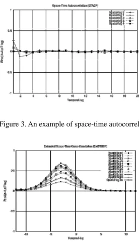
The first step of Box-Jenkins’ model approach is to identify an appropriate model type/model orders for a given dataset. Based on the behavior of the space-time autocorrelation/partial autocorrelation (as shown in the Figure 3 and 4), the model type/order can be determined artificially or automatically by software.
Figure 5. An example of parameter estimation Figure 3. An example of space-time autocorrelation
Once the model type, order, and parameter estimates have been obtained, the acquired mode can be used to forecast or to analyze the future behavior of the system of interest. However, to prevent unacceptable forecasting errors, we have to check if the fitted model is appropriate. These checking methods are called diagnostic checks. There are various methods provided to check the model adequacy, i.e. space-time autocorrelations of the residuals, statistical significance testing, and goodness measures (i.e. Akaike’s Information Criterion or AIC and Bayesian Information Criterion or BIC).
Figure 4. An example of space-time cross correlation
Inadequacy of a candidate model will be unveiled in the form of significant space-time correlations among the residuals. Furthermore, a tentative model needs to be checked to see if it is unduly complex. The statistical significance of model parameters is evaluated for this purpose. In addition to the analyses of residual’s autocorrelations and statistical significance, AIC/BIC measures are also very useful. In most practical cases, space-time autocorrelations do not obviously reveal the type/orders. In such situations, it is not easy to determine the type/orders by observing the behaviors of these autocorrelations. AIC/BIC were extended to space-time cases and implemented in IEAST. Both AIC and BIC are relative measures. They are useful when select the best model out of many candidates.
In IEAST, they are especially useful when using the IEAST programming environment (interpreter mode) in which iterative test of AIC/BIC on different models is a powerful method to pick a good model for a given dataset out of lots of candidates automatically by STARMA modeling scripts.
After the candidate model is decided, the next step is to find a set of parameters for the model. This is estimation stage. It is the most time-consuming stage. The stage is implemented with the maximum likelihood estimates (MLE). In IEAST, we have designed not only the algorithms for estimating model parameters, but also the algorithms for estimating spatial weighting structure.
Because of nonlinear nature of STMA and mixed models, we have to use a nonlinear optimization algorithm to find the estimates.
Marquardt’s algorithm [3] was chosen to implement the nonlinear optimization of model parameter estimates. During the optimization process, we added an extra stage, pre-estimation, right before the estimation stage, to calculate the appropriate initial starting points for the optimization algorithm.
Hanan-Rissanen algorithm [2] is used for the pre-estimation stage. (e.g. Figure 5)
In IEAST, the programming environment provided is an interpreter. In general, an interpreter parses and executes requested actions in every statement line by line in a script. This enviroment provides a method using scripts to compose a modeling job. From the point of view of functionalities provided, interpreter is parallel to
Figure 7. Assignment of spatial order definition menu-driven environment. Each of them can
separately works well. The interpreter gives an even more powerful ability for modeling STARMA processes. Combining with the suggested STARMA modeling procedure, under the interpreter users can construct a complete and efficient modeling flow with maximum flexibility. The interactive response and attention from users are not necessary.
Beside space-time datasets, another essential part of preparation for modeling is to specify a spatial correlation structure for a dataset (in practice, it is a definition of set of weight matrices). The specification describes the relative spatial relations among cells (e.g. Figure 7), including the definition of spatial orders, weighting distributions, and spatial dimension. In most of practical cases, spatial correlation structures are isotropic (or directionless).
Thus, once the definition of spatial order (or lags) is given, IEAST can generate an appropriate set of weight matrices for the isotropic structure. IEAST provides a very flexible method for users to assign a spatial structure step-by-step and automatic translation to reduce the burden of manual transformations. The users only need to assign a spatially relative correlation structure, and then the corresponding weight matrices will be generated.
The targets for STARMA modeling are space-time datasets. There are two global variable which can be loaded into IEAST, i.e. the major variable (Z) and the secondary variable (Y). The major variable is involved in all space-time analyses and modeling. The secondary variable is needed only while evaluating the relation between the major variable and other covariate.
The only file format from which IEAST can directly retrieve is the octave-formated data file, which is a standard format for storing variables in GNU Octave. Besides, IEAST also provides some transformations from other data formats to octave format for future uses. Currently, the tab-separated text file with various formats are allowed to be imported to IEAST.
The entire structure and functionalities of IEAST can be divided into 7 categories (these categories are listed in the menu of IEAST as shown in Figure 8):
1. Setup: this includes dataset retrieving, file format translation, assignment of spatial correlation structure.
After datasets retrieved from file, for most cases, we need to make some transformation or preprocessing in order to make space-time series satisfy some statistical conditions (e.g. statistical stationarity). In IEAST, there are many preprocessing functionalities provide for this purpose. In Figure 6, a spatial is found by the functionality in the preprocessing.
2. Preprocessing: including de-seasonalization, differencing, data sub-sampling, smoothing, filling missing data, data filtering with given STARMA model.
3. Correlation analysis: including space-time autocorrelation/partial autocorrelation, cross correlation between two space-time variables, and correlation plotting.
4. Model identification: including automatic identification, artificial identification, and parameter masking.
5. Parameter estimation: including linear estimation, robust non-linear estimation, estimation of spatial correlation structures.
6. Diagnostic analysis: including evaluations of statistical significance of parameters, AIC/BIC model goodness measures, residual’s autocorrelation/partial autocorrelation.
7. Interpreter environment: as shown in Figure 9.
Figure 6. Finding spatial trend using preprocessing
Figure 8. First page of IEAST menu
Figure 9. An example of a complete modeling script
Future Development
Future developments will mainly on the transferring from text-mode interface to window-based interface to make the software more easy-to-use for users and providing the ability to interface with GIS system.
A comprehensive user manual can be found on the web site:
http://dns2.asia.edu.tw/~leecheng/do c/ieastman.pdf
Acknowledgement
This study was supported by the Michigan Agricultural Experiment Station, Michigan State University, USA.
Reference
1. Box, G. E. P. and Jenkins, G. M. (1970). Time Series Analysis: Forecasting and Control.
Holden-Day, San Francisco.
2. Hannan, E.J. and Rissanen, J. Recursive estimation of mixed auto-regressive moving average order. Biometrika, 69:81-94, 1982.
3. Marquardt, D.W. An algorithm for least squares estimation of nonlinear parameters. Journal of the Society of Industrial and Applied Mathematics, 11:431-441, 1963.
4. Pfeifer, P. E. Spatial-Dynamic Modeling (Unpublished Ph.D. dissertation). Georgia Institute of Technology, Atlanta, Georgia, 1979.
5. Pfeifer, P.E. and Deutsch, S.J. A three-stage iterative procedure for space-time modeling.
Technometrics 22(1), 35-47, 1980.
6. Pfeifer, P.E. and Deutsch, S.J. A comparison of estimation procedures for the parameters of the STAR model. Communications in Statistics - Simulation and Computation, B9 (3):255-270, 1980.