附最低保證變額年金保險最適資產配置及準備金之研究 - 政大學術集成
54
0
0
全文
(2) 謝辭 兩年的研究所生涯即將劃上句點,準備邁向人生的下一階段,走過人生當中最充實 且愉快的兩年,最要感謝的就是我的指導教授黃泓智老師,與李永崇老師。黃老師不僅 在論文上引導我的方向,也分享許多人生經歷,讓我受益良多;永崇學長在這一年中, 百忙之中仍花了許多時間指引我的論文方向,到口試之前,又花了許多時間幫忙我補救 我不足的英文,在此,要特別感謝永崇學長,最後,感謝王儷玲老師、余清祥老師已及. 政 治 大. 王昭文老師在口試中也提供許多寶貴的意見,讓本論文能更臻完善。. 立. ‧ 國. 學. 在研究所的兩年中,除了老師的教誨,最令人開心的事情,莫過於認識一群志同道 合的朋友,有你們的幫忙,我才能在兩年的風風雨雨中安全的度過,讓離家在外的我不. ‧. 覺得孤單,最後,要最感謝舒雲的貼心包容,我的內心充滿感激與珍惜。. y. Nat. io. sit. 最後,當然要感謝我的父母與姐姐妹妹,有你們在背後的默默支持,我才能無後顧. n. al. er. 之憂,謝謝你們的無私付出。. Ch. engchi. i n U. v. 陳尚韋 謹誌於 國立政治大學風險管理與保險學研究所 民國一百年七月.
(3) 摘要 附最低保證投資型保險商品的特色在於無論投資者的投資績效好壞,保險金額皆 享有一最低投資保證,過去關於此類商品的研究皆假設標的資產為單一資產,或依固 定比例之投資組合,並沒有考慮到投資人自行配置投資組合的效果,但大部分市售商 品中,投資人可以自行配置投資標,此情況之下,保險公司如何衡量適當的保證成本 即為一相當重要之課題。 本研究假設投資人風險偏好服從冪次效用函數,並假設與保單所連結之投資標的 有兩種資產,一為具有高風險高報酬的資產,另一為具有低風險低報酬之資產,在每 個保單年度之初,投資人可以選擇配置在兩種資產之比例,我們運用黃迪揚(2009)所提. 政 治 大. 出的動態規劃數值解之方法,計算出在考慮投資人自行配置資產之下,保證成本將會. 立. 比固定比例之投資高出12個百分點。. ‧ 國. 學. 此外,為了瞭解在不同資產報酬率的模型之下,保證成本是否會有不一樣的結 論,除了對數常態模型之外,我們假設高風險資產與低風險資產服從ARIMA-. ‧. GARCH(Autoregressive Integrated Moving Average-Generalized Autoregressive Conditional. y. Nat. Heteroscedastic )模型,並得到較高的保證成本。. n. al. er. io. 效用函數、變額年金. sit. 關鍵詞:附投資保證提領保險商品、動態規劃求解、ARIMA-GARCH 模型、冪次. Ch. engchi. i n U. v.
(4) Abstract The main characteristic of variable annuities (VA) with minimum benefits is that the benefit will be guaranteed. Previous literatures assume a specific underling asset return process when considering the guaranteed cost of VA; but they do not consider the portfolio choice opportunity of the policyholders. However, it is common for policyholders to rebalance his portfolio in many types of VA products. Therefore it‟s important for insurance companies to apply an approximate method to measure the guaranteed cost. In this research, we assume that there are two potential assets in policyholders‟ portfolio; one with high risk and high return and the other one with low risk and low return. The utility function of the policyholder is assumed to follow a power utility. We consider the asset. 政 治 大 benefits, finding that the guaranteed cost will increase 12% compared with 立. allocation effect on the guaranteed cost for a VA with guaranteed minimum withdrawal a specific. underling asset.. ‧ 國. 學. The model effect of the asset return process is also examined by considering two different asset processes, the lognormal model and ARIMA-GARCH model. The solution of. ‧. dynamic programming problem is solved by the numerical approach proposed by Huang. io. .. n. al. Keyword:GMWB、dynamic. Ch. Utility Function、Variable Annuity. y er. GARCH model is greater than the lognormal model.. sit. Nat. (2009). Finally we get the conclusion which the guaranteed cost given by the ARIMA-. v ni. programming、ARIMA-GARCH. engchi U. model、Power.
(5) Catalog CATALOG ........................................................................................................................................................I LIST OF TABLE ..........................................................................................................................................II LIST OF FIGURE .............................................................................................................................................III 1 INTRODUCTION .......................................................................................................................................... 1 2 LITERATURE REVIEW .......................................................................................................................... 4 2.1 PRICING OF GMWB ...................................................................................................................................... 4. 治 政 大 3 METHODOLOGY .......................................................................................................................................... 8 立 3.1 D G M B ......................................................................................................... 8 2.2 BASIC TYPE OF GUARANTEED PRODUCT ........................................................................................................ 6. UARANTEED. INIMUM ENEFIT. 學. ‧ 國. ESIGN OF. 3.2 ASSET MODEL ............................................................................................................................................. 10 3.3 UTILITY FUNCTION ...................................................................................................................................... 12. ‧. 3.4 PARAMETER ESTIMATION ............................................................................................................................. 12 4 NUMERICAL RESULTS ........................................................................................................................ 18. y. Nat. sit. 4.1 RESULT OF SIMULATION ..................................................................................................................................... 18. er. io. 4.2 ANALYST OF RESULT .......................................................................................................................................... 21 4.3 THE IMPROVEMENT OF THE POLICYHOLDER’S EXPECTED UTILITY ................................................................................ 28. n. al. i n U. v. 4.4 THE RESULT OF VA WITH GMMB ....................................................................................................................... 29. Ch. engchi. 5 SENSITIVITY ANALYSIS...................................................................................................................... 31 5.1 SENSITIVITY ANALYSIS OF. THE RISK-AVERSE PARAMETER ......................................................................................... 31. 5.2 SENSITIVITY ANALYSIS OF MODEL ......................................................................................................................... 35 6. CONCLUSION ................................................................................................................................. 37. REFERENCE .................................................................................................................................................. 39 APPENDIX A. THE DATA OF THE MAIN FIVE INDEXES IN U.S. ......................................................................... 41 APPENDIX B. THE DECISION TABLE OF GMMB .............................................................................................. 43. I.
(6) List of Table TABLE 1.1:TOTAL SALES OF INDIVIDUAL ANNUITIES IN THE U.S. ,2001-2010($ BILLIONS) ................................. 2 TABLE 1.2 ELECTION RATE OF LIVING BENEFIT(14 CARRIERS PROVIDED) ......................................................... 2 TABLE 3.1 THE STATISTICS DATA OF DOW JONES INDUSTRIAL AVERAGE INDEX AND NASDAQ COMPOSITE .... 14 TABLE 3.2 THE K-S TEST OF DOW JONES INDUSTRIAL AVERAGE INDEX AND NASDAQ COMPOSITE................. 15 TABLE 3.3 THE SUMMARY OF ADF TEST OF DOW JONES AND NASDAX ...................................... 16 TABLE 3.4 THE ORDER OF ARIMA-GARCH ..................................................................................................... 16. 政 治 大 TABLE 4.1 THE DECISION TABLE OF OUR BENCHMARK (THE WEIGHT IS PROPORTION OF HIGH RISK ASSET) .. 19 立 TABLE 3.6 THE COEFFICIENT OF ARIMA-GARCH ............................................................................................ 17. ‧ 國. 學. TABLE 4.2 THE INITIAL WEIGHT OF 100 TIMES OF 10000 DIFFERENT SENARIOS. ............................................ 21 TABLE 4.3 THE EXPLAIN OF DECISION TABLE ................................................................................................. 23. ‧. TABLE 4.4 THE COST IN 10000 DIFFERENT SCENARIOS .................................................................................. 24 TABLE 4.6 THE SUMMARY OF EXPECTED UTILITY .......................................................................................... 28. y. Nat. sit. TABLE 4.7 THE SUMMARY OF EXPECTED UTILITY .......................................................................................... 30. er. io. GMMB ....................................................................................................................................................... 30. al. n. v i n C h WEIGHT ANDUFIXED INITIAL AND AVERAGE WEIGHTS 32 TABLE 5.2 THE DIFFERENCE COST BETWEEN VARIABLE engchi TABLE 5.1 THE SUMMARY OF DIFFERENT RISK-AVERSE PARAMETER IN 10000 SCENARIOS ............................ 32. TABLE 5.3 THE OTHER DIFFERENCE BETWEEN VARIABLE WEIGHT AND FIXED INITIAL AND AVERAGE WEIGHT 33 TABLE 5.4 (THE DIFFERENCE OF THE COST OF GMWB BETWEEN LOGNORMAL MODEL AND ARIMA-GARCH MODEL) ....................................................................................................................................................... 35 TABLE 5.5 THE DIFFERENCE OF EXPECTED COST BETWEEN DIFFERENT ASSET MODELS .................................. 36 TABLE APPENDIX A.1 THE NORMAL TEST OF MAIN FIVE INDEXES IN U.S ( EXPIRE AT 2010/12) ...................... 41 TABLE APPENDIX A.2 ANNUALIZED RETURN AND VOLATILITY OF FIVE MAIN INDEXES ON MONTHLY INFORMATION............................................................................................................................................. 41 TABLE APPENDIX A.3 CORRELATION TABLE OF FIVE MAIN INDEXES ON MONTHLY INFORMATION ................. 42. II.
(7) List of Figure FIGURE 3.1 THE HISTOGRAM OF NASDAQ INDEX MONTHLY RETURN FROM 1990/1 TO 2010/12 ................... 13 FIGURE 3.2 THE HISTOGRAM OF NASDAQ INDEX MONTHLY RETURN FROM 1990/1 TO 2010/12 ................... 14 FIGURE 4.1 THE WEIGHTS OF HIGH-RISK ASSET RANK BY THE ACCOUNT VALUE IN EACH PERIOD .................. 27 FIGURE 4.2 THE WEIGHT OF 5TH, 25TH, 50TH , 75TH, 95TH RANK BY THE WEIGHTS IN EACH PERIOD ................. 27 FIGURE 4.3 THE DIFFERENCE OF UTILITY BETWEEN OUR BENCHMARK AND THE FIXED WEIGHT .................... 29 FIGURE 4.4 THE AVERAGE WEIGHT RANKED BY THE ACCOUNT VALUE IN EACH PERIOD OF VA WITH GMMB . 30. 治 政 FIGURE 5.2 THE EXPECTED COST IN DIFFERENT UTILITY PARAMETER COMPARED 大 TO FIXED AVERAGE WEIGHT 立 ................................................................................................................................................................... 34 FIGURE 5.1 THE EXPECTED COST IN DIFFERENT UTILITY PARAMETER COMPARED TO FIXED INITIAL WEIGHT . 33. ‧. ‧ 國. 學. FIGURE 5.3 THE AVERAGE WEIGHT AT EACH TIME GIVEN DIFFERENT UTILITY PARAMETER ............................ 34. n. er. io. sit. y. Nat. al. Ch. engchi. III. i n U. v.
(8) 立. 政 治 大. ‧. ‧ 國. 學. n. er. io. sit. y. Nat. al. Ch. engchi. i n U. v.
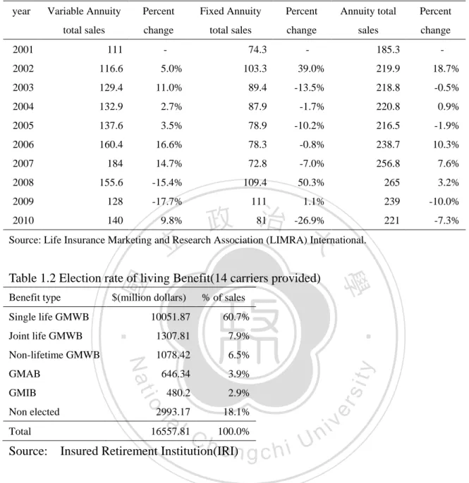
(9) 1 Introduction Variable annuities (VA) have two features of life insurance and investment. The benefits depend on the performance of the investment portfolio selected by the policyholders. However, the policyholders may take more investment risk simultaneously. This is one of the biggest differences between VA and the traditional life insurance policy. In the U.S., variable annuities assets reached an historical peak of 1.6 trillion at the first quarter of 2011. The total. 政 治 大 representing a 9.8% increase (see Table 1.1). About 81.9% of variable annuities were 立. sales of variable annuity in 2010 were $140 billion , up from $128 billion in the previous year,. ‧ 國. 學. guaranteed variable annuities and about 75.1% have the GMWB (guaranteed minimum withdrawal benefits) feature in the first half of 2010 from 14 carriers provided1 (see Table. ‧. 1.2). Popular types of guaranteed benefit include Guaranteed Minimum Withdrawal Benefit. sit. y. Nat. (GMWB), Guaranteed Minimum Accumulation Benefit (GMAB), and Guaranteed Minimum. io. al. er. Income Benefit (GMIB); Hardy (2003) has described these types of products, and we will. n. introduce these types of variable annuity on the next chapter in detail.. Ch. engchi. i n U. v. “As the first wave of the 79 million baby boomers (from 1946 to 1964) reached sixtyfives years old, guaranteed retirement income strategy was believed to continue to grow” said Insured Retirement Institute (IRI) President and CEO Cathy Weatherford. Recent IRI research shows that 92% of boomers who own an annuity have stronger confidence in the financial stability than those who do not, so variable annuities has still great potential to grow.. 1. The 14 carriers include Jackson National, AXA Financial, Aegon / Transamerica, Allianz, John Hancock, Pacific Life Protective, Hartford, Guardian, Mass Mutual, Principal, Penn Mutual, Cuna, Symetra, and Integrity.. 1.
(10) Table 1.1:Total Sales of individual annuities in the U.S. ,2001-2010($ billions) year. Variable Annuity. Percent. Fixed Annuity. Percent. Annuity total. Percent. total sales. change. total sales. change. sales. change. 2001. 111. -. 74.3. -. 185.3. 2002. 116.6. 5.0%. 103.3. 39.0%. 219.9. 18.7%. 2003. 129.4. 11.0%. 89.4. -13.5%. 218.8. -0.5%. 2004. 132.9. 2.7%. 87.9. -1.7%. 220.8. 0.9%. 2005. 137.6. 3.5%. 78.9. -10.2%. 216.5. -1.9%. 2006. 160.4. 16.6%. 78.3. -0.8%. 238.7. 10.3%. 2007. 184. 14.7%. 72.8. -7.0%. 256.8. 7.6%. 2008. 155.6. -15.4%. 109.4. 50.3%. 265. 3.2%. 2009. 128. -17.7%. 111. 1.1%. 239. -10.0%. 2010. 140. 9.8%. 221. -7.3%. 政 81治 -26.9% Source: Life Insurance Marketing and Research Association (LIMRA)大 International. 立. 7.9%. 1078.42. 6.5%. 646.34. 3.9%. 480.2. 2.9%. al. 2993.17. n. Non elected Total. Ch. 16557.81. Source:. 18.1% 100.0%. engchi. Insured Retirement Institution(IRI). y. 1307.81. io. GMIB. 60.7%. sit. GMAB. 10051.87. Nat. Non-lifetime GMWB. % of sales. ‧. Joint life GMWB. $(million dollars). er. Single life GMWB. ‧ 國. Benefit type. 學. Table 1.2 Election rate of living Benefit(14 carriers provided). -. i n U. v. When insurance companies launch guaranteed product, insurers are no longer transferring all investment risk to policyholders. They face the risk that the account value is lower than the guaranteed value. Because the investment behavior of the policyholders will affect the guaranteed cost, it becomes important for insurance companies to employ a correct method to calculate cost.. 2.
(11) This study adopts dynamic programming method by creating asset allocation decision table to price the guaranteed cost of variable annuities with guaranteed minimum benefit. This method is proved by Huang(2009). Although there are many researches which has offered several methods to price the products in the past, all of them assume that the underlying asset is a single asset or a fixed portfolio and do not consider the asset allocation opportunity of the policyholders. In this research, we calculate the guaranteed cost of VA with guaranteed minimal benefits when the policyholders have the right to rebalance his portfolio.. 立. 政 治 大. ‧. ‧ 國. 學. n. er. io. sit. y. Nat. al. Ch. engchi. 3. i n U. v.
(12) 2 Literature review The first research related to the pricing of variable annuities with guaranteed minimum benefit is Brennan and Schwartz (1976; 1979). They use Black-Scholes option theory to do the pricing and investment strategy of GMMB (guaranteed minimum maturity benefit) with single premium first. Then Brennan and Schwartz (1979) argues that the guaranteed product with level premium does not have closed form solution, therefore numerical simulation is. 政 治 大 simulation method to calculate the fair value for the product with level premium. Boyle and 立 required. In 1990s, Delbacn (1990) uses the martingale pricing method and the numerical. ‧ 國. 學. Schwartz (1997), Boyle and Hardy (1997) and Aase and Persson (1997) use methods of evaluation in financial economics to price of the guaranteed minimum benefit. Milevsky and. ‧. Posner (2001) calculate the guaranteed fee for GMDB. Then Coleman el al. (2005, and 2007). er. io. sit. y. Nat. provide several analyses for GMDB under different hedging and data generating models. n. al 2.1 Pricing of GMWB Ch. engchi. i n U. v. Bakshi and Madan (2002), Nielsen and Sandmann (2003) and Dhaene (2001) use different numerical methods by applying the concept of Asian option to price the VA of GMWB. Milvwsky and Salisbury (2006) develop static and dynamic methods for assessing the cost and value of variable annuities with GMWB. First, the static approach assumes that the policyholder will hold the policy until maturity, and shows that the product can be separated into a Quanto Asian Put and a generic term-certain annuity. Second, the dynamic approach proposes that the policyholder will terminate the policy when the expected present. 4.
(13) value of fees the insurer charges exceeds the expect present value of guarantee. It is similar to price an American put. They conclude that the guaranteed cost of the policy is about 73 to 160 basis points of the asset. Dai el al. (2008) develop a singular stochastic control model for pricing variable annuities with GMWB and allow the policyholder to choose his own withdrawal strategy under both continuous and discrete frameworks. Chen el al. (2008) considers the effect of mutual fund fees and sub-optimal withdrawal behavior when calculate the price of VA with GMWB. Peng el al. (2009) focus on the interest rate risk and develops model formulations of the ruin probability and price function, and furthermore derives. 政 治 大. analytic approximation solution to the function. Turnbull (2008) prices the guaranteed fee by. 立. the delta hedge strategy for GMWB, and shows that the strategy may incur a numerous lose in. ‧ 國. 學. the financial tsunami. Bascinello et al. (2009) develop the life insurance contracts with surrender guarantees, and Holz et al. (2007) price the GMWB for life riders. Liu (2010). ‧. calculates the expected cost of VA with GMWB by three different approaches of delta hedge,. Nat. sit. y. delta-gamma hedge and semi-static hedge. However, all of the above literatures assume that. n. al. er. io. the underlying asset is a single asset or a fixed portfolio, and do not consider the asset. i n U. v. allocation opportunity of the policyholder. In this research, we consider the asset allocation. Ch. engchi. effect and price the variable annuity with guaranteed minimal benefit.. Huang (2009) develop a numerical method for solving dynamic programming problem by creating asset allocation decision table. We use the same dynamic programming approach to price GMWB when considering the optimal investment strategy for policyholders.. 5.
(14) 2.2 Basic type of guaranteed product Popular types of variable annuity with guaranteed minimum benefit include Guaranteed Minimum Withdrawal Benefit (GMWB), Guaranteed Minimum Accumulation Benefit (GMAB), and Guaranteed Minimum Income Benefit (GMIB).. The GMIB (Guaranteed Minimum Income Withdrawal) guarantees a minimum compounding rate and a minimum level of annuity income payment. This benefit is only. 政 治 大. applicable if the policyholder annuitizes the contract.. 立. ‧ 國. 學. The GMAB (Guaranteed Minimum Accumulation Withdrawal) guarantees a minimum account value in the end of a specified period. If the asset value is greater than the guaranteed. ‧. value, the policyholder has the right to renew the contract at a new guaranteed level which is. Nat. er. io. sit. y. the same as the asset value at that time.. Guaranteed Minimum Withdrawal Benefit (GMWB). n. al. Ch. engchi. i n U. v. The GMWB guarantees the policyholder make periodic withdrawals regardless of the impact of poor market performance on the account value. There is a maximum annual withdrawal amount usually defined as 7% of premium, and the benefit period could last up to 15 years or more. GMWB can be divided into two parts. The first part is guaranteed withdrawal balance (GWB). The GWB represents that the policyholder can at least receive a guaranteed minimum benefit, and it usually equals to the amount of the premium paid or 105% of the premium paid. The second part is Maximum Annual Withdrawal Amount (MAWA). The MAWA stands for the maximum withdrawal amount, and usually equal to 7%. 6.
(15) of the GWB. Two of the popular types are the GMWB for life (or lifetime GMWB) and the joint life GMWB. The GMWB for life guarantees that the policyholder can withdraw a percentage (e.g. 5%) of the premium paid from age 65 to life and the joint life GMWB guarantees benefit payments to the living spouse.. 立. 政 治 大. ‧. ‧ 國. 學. n. er. io. sit. y. Nat. al. Ch. engchi. 7. i n U. v.
(16) 3 Methodology In this chapter, we introduce and explain our design of guaranteed minimum benefit, utility function model of the policyholder and the optimal strategy.. 3.1 Design of Guaranteed Minimum Benefit. 立. 政 治 大. ‧ 國. 學. We consider a T-year variable annuity with guaranteed minimum benefit. For simplicity,. ‧. we assume that there are two assets, and the policyholder can make asset allocation decision on his portfolio in the beginning of each year. One of two assets has high return and high risk. y. Nat. n. al. er. io. sit. and the other has low return and low risk. The following are the definitions of the symbols:. Ch. engchi. i n U. v. in the beginning of year t. : the market value of separate account in the end of year t : the guaranteed value of separate account at the end of year t : the premium at time t m: the fee ratio of account d: withdrawal rate, a percentage of single premium. Guaranteed minimum maturity Benefit We consider a T-year variable annuity with guaranteed minimum maturity benefit. After T. 8.
(17) year, the policyholder will get the account value or the guaranteed value whichever is greater.. The market value of account at time. is. At the end of year T, the policyholder can receive:. 政 治 大. Guaranteed minimum withdrawal Benefit. 立. ‧ 國. 學. We consider a T-year variable annuity with single premium guaranteed minimum withdrawal benefit. The policyholders will withdraw a percentage of the single premium at. ‧. the end of each year until the guaranteed value becomes zero.. :. n. er. io. al. sit. y. Nat. The market value of account at time. Ch. engchi. The guaranteed value at time :. At the end of year T, the policyholder can receive:. 9. i n U. v.
(18) 3.2 Asset Model In order to avoid asset model error, we assume that assets are subject to two different models, log-normal model and the Autoregressive Integrated Moving Average-Generalized Autoregressive Conditional Heteroscedastic (ARIMA-GARCH) model.. Lognormal model. 政 治 大. Lognormal model assumes that return of asset after taking logarithmic will follow Normal. 立. distribution. The dynamic processes of two assets are. y. sit. n. er. io. at P measure :standard Brownian motion. al. ‧. ‧ 國. 學. „1‟ represent high risk asset and „2‟ represent low risk asset at time t. Nat. k=1,2. Ch. engchi. i n U. v. Autoregressive Integrated Moving Average-Generalized Autoregressive Conditional Heteroscedastic (ARIMA-GARCH) model. First, Morgan (1976) shows that the return of equity has a heterogeneous phenomenon which represents the volatile of the equity return will change with time. Mandelbrot (1963) and Fama (1965) propose the distribution of financial time series has the characteristics of. 10.
(19) leptokurtic, fat tail and non-lognormal distribution; and its volatile has the phenomenon of volatility clustering. As a result, Engle (1982) develops ARCH (Autoregression Conditional Heteroskedaticity) model. The main characteristic of this model is taking the residual of lag periods as a conditional variance; the model later gets the empirical support from the market data in UK. After this, Bollerslev (1986) expands ARCH model to GARCH model (Generalized Autoregression Conditional Heteroskedaticity), and shows GARCH model can capture all the features of the volatile. Therefore we use this model to fit the linked assets in our study. The asset process of ARIMA(p, e, q)-GARCH( j , k) model :. 立. 政 治 大. ‧. ‧ 國. 學 er. io. sit. y. Nat. al. v. n. k=‟1‟,‟2‟ „1‟ represents high risk asset and „2‟ represents low risk asset. Ch. engchi. i n U. p: the order of the autoregressive part e: the order of the integrated part q: the order of the moving average part of asset k and follow normal distribution of k in the GARCH model j: the order of the autoregressive part of volatility k: the order of the moving average part of volatility. 11.
(20) 3.3 Utility function The VAs with GMWB guarantee the policyholder receive fixed withdraws every periods expect the last period, so the policyholder will get the same utility in the first (T-1) periods. As a result, we only need to consider the utility function the last period. In our research, we assume that the policyholder is risk-averse and the utility function follows power utility function:. 立. 政 治 大. W:Accout value of the policyholder. ‧ 國. 學. The power utility function is constant relative risk aversion. No matter how much wealth. ‧. the policyholder has, the attitude of financial risk will not change; this means that the proportion of the portfolio in each asset class will not change with the dollar amount of the. y. Nat. n. al. Ch. engchi. er. io. portfolio to maximize the expected utility at time T.. sit. portfolio. At the beginning of each year, the policyholder will choose a best investment. i n U. v. 3.4 Parameter estimation In this section, we explain how we choose the return and volatility of asset in the lognormal model and the ARIMA-GARCH model. The linked assets of VA are usually mutual equity funds or mutual bond funds in the market. In order to meet the actual situation, we. 12.
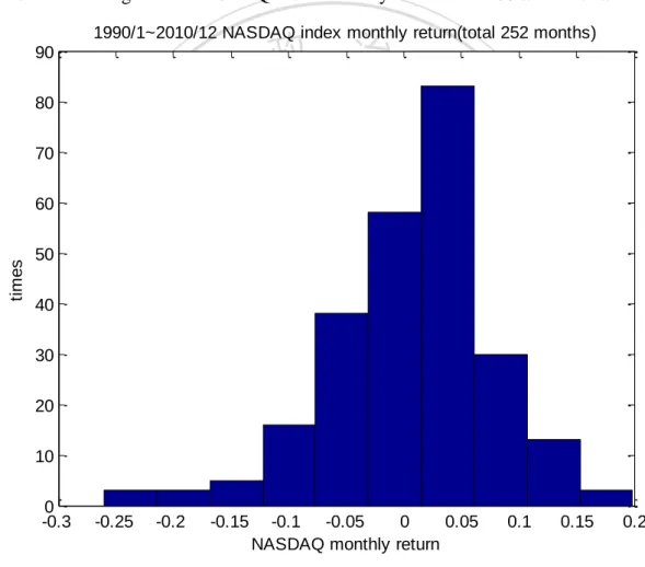
(21) assume two indexes in the U.S. as two linked mutual equity funds in our paper. First, we pick five indexes2 in the U.S. and choose two more suitable indexes from the five indexes, and find the Dow Jones Industrial Average index and the NASDAQ Composite index are more suitable because of the following two reasons; First,the correlation between these two indexes is the lowest among other indexes in U.S . Second, their return and volatility are significantly different. Then we choose the period from 1990/1~2010/12 to match our model. Figure 3.1 The histogram of NASDAQ index monthly return from 1990/1 to 2010/12. 政 治 大. 1990/1~2010/12 NASDAQ index monthly return(total 252 months) 90. 立. 80. ‧ 國. ‧. io. y. al. n. 30. sit. 40. er. 50. Nat. times. 60. 學. 70. 20. Ch. engchi. i n U. v. 10 0 -0.3. -0.25. -0.2. -0.15. -0.1 -0.05 0 0.05 NASDAQ monthly return. 2. 0.1. 0.15. 0.2. The five indexes are Dow Jones Industrial Average index , NASDAQ Composite index, Russell 2000, S&P500, and S&P100.. 13.
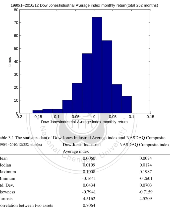
(22) Figure 3.2 The histogram of NASDAQ index monthly return from 1990/1 to 2010/12 1990/1~2010/12 Dow JonesIndustrial Average index monthly return(total 252 months) 80 70 60. times. 50 40 30. 立. 20. ‧ 國. ‧. 0 -0.2. 學. 10. 政 治 大. -0.15 -0.1 -0.05 0 0.05 0.1 Dow JonesIndustrial Average index monthly return. Nat. sit. y. 0.15. Mean Median Maximum Minimum Std. Dev. Skewness Kurtosis Correlation between two assets. Dow Jones Industrial Average index. Ch. er. al. n. 1990/1~2010/12(252 months). io. Table 3.1 The statistics data of Dow Jones Industrial Average index and NASDAQ Composite. n U engchi 0.0060 0.0109 0.1008 -0.1641 0.0434 -0.7941 4.5162 0.7064. 14. iv. NASDAQ Composite index 0.0074 0.0174 0.1987 -0.2601 0.0703 -0.7159 4.5209.
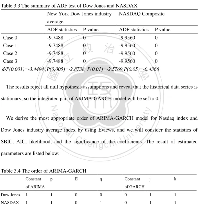
(23) Table 3.2 The K-S test of Dow Jones Industrial Average index and NASDAQ Composite Dow Jones Industrial Average index. 1990/1~2010/12(252 months). The statistic of K-S test. NASDAQ Composite index. 0.0684. 0.0758. ※. Lognormal model Normal test. 治 政 follows the Normal distribution. The null hypothesis and alternative 大 hypothesis are 立. In this paper, we use Chi-square test to test whether the logarithm of historical return rates. ‧. ‧ 國. 學. Nat. n. al. er. io. ARIMA-GARCH model. sit. that dynamics of assets can be captured by lognormal distribution.. Uni-root test( stationary test). y. The result doesn‟t reject the null hypothesis under the 95% confident level and we can say. Ch. engchi. i n U. v. We use ADF (Augmented Dickey-Fuller) to test whether the time series after taking logarithm of historical return rates is a stationary series. The null hypothesis and alternative hypothesis are:. Case 0: DGP(Data Generating Process) and estimated model contain no deterministic trends. 15.
(24) Case 1: DGP contains no deterministic time trend but estimated model includes a constant and a time-trend Case 2: DGP contains a constant or a time trend. Estimated model includes both a constant and a time trend Case 3: DGP and estimated model contain a constant Table 3.3 The summary of ADF test of Dow Jones and NASDAX. Case 0 Case 1 Case 2 Case 3. New York Dow Jones industry average. NASDAQ Composite. ADF statistics. P value. ADF statistics. P value. -9.7488 -9.7488 -9.7488 -9.7488. 0 0 0 0. -9.9560 -9.9560 -9.9560 -9.9560. 0 0 0 0. 政 治 大. 立. ‧ 國. 學. ※P(0.001)=-3.4494 ,P(0.005)=-2.8738, P(0.01)=-2.5769,P(0.05)=-0.4366 The results reject all null hypothesis assumptions and reveal that the historical data series is. ‧. stationary, so the integrated part of ARIMA-GARCH model will be set to 0.. sit. y. Nat. io. al. er. We derive the most appropriate order of ARIMA-GARCH model for Nasdaq index and. iv n U coefficients.. n. Dow Jones industry average index by using Eviews, and we will consider the statistics of. Ch. engchi. SBIC, AIC, likelihood, and the significance of the. The result of estimated. parameters are listed below: Table 3.4 The order of ARIMA-GARCH Constant. p. E. q. of ARIMA. Constant. j. k. of GARCH. Dow Jones. 1. 1. 0. 0. 0. 1. 1. NASDAX. 1. 1. 0. 1. 0. 1. 1. 16.
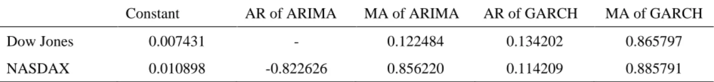
(25) Table 3.6 The coefficient of ARIMA-GARCH Constant. AR of ARIMA. MA of ARIMA. AR of GARCH. MA of GARCH. Dow Jones. 0.007431. -. 0.122484. 0.134202. 0.865797. NASDAX. 0.010898. -0.822626. 0.856220. 0.114209. 0.885791. Because our data is monthly return of the two indexes, we simulate 180 months in 10000 different scenarios. Based on the data of 180 months, we generate 15 annual return by multiplying every 12 monthly return.. 立. 政 治 大. ‧. ‧ 國. 學. n. er. io. sit. y. Nat. al. Ch. engchi. 17. i n U. v.
(26) 4 Numerical results In this chapter, we create decision table for optimal asset allocation and calculate the cost of variable annuities with guaranteed minimum withdrawal benefit and guaranteed minimum maturity benefit by the Monte-Carlo method proposed by Huang (2009).. 4.1 result of simulation 政 治 大 We assume a benchmark that立 a policyholder buys a 15-year variable annuity with GMWB,. ‧ 國. 學. the single premium is 100 dollars and the withdrawal rate is 7%. The policyholder is a riskaverse person with power utility function, and the relative risk aversion parameter of the. ‧. policyholder is 1. The expected annualized return and the annualized volatility of low risk. Nat. sit. y. asset after taking logarithmic are 0.0735 and 0.1496 respectively. The expected annualized. n. al. er. io. return and the annualized volatility of on high-risk asset after taking logarithmic are 0.0937. i n U. v. and 0.2429; and the correlation between the two assets is 0.7064.. Ch. engchi. In order to reduce the variation generated by the simulation, we repeat 100 times the simulation of the different 10000 scenarios, and get 100 different decision tables. Then we use the arithmetic average of 100 decision tables as our decision table of benchmark. The decision table and the summary of our benchmark are listed below:. 18.
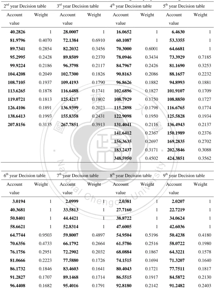
(27) Table 4.1 The decision table of our benchmark (The weight is proportion of high risk asset) 2nd year Decision table Account. 3rd year Decision table. Weight. Account. value. 4th year Decision table. Weight. Account. value. 5th year Decision table. Weight. Account. value. Weight. value. 28.0007. 1. 16.0652. 1. 6.4630. 1. 81.9796. 0.4070. 72.1384. 0.6910. 60.1087. 1. 53.3355. 1. 89.7341. 0.2854. 82.2032. 0.3456. 70.3000. 0.6001. 64.6681. 1. 95.2995. 0.2428. 89.8509. 0.2370. 78.0946. 0.3434. 73.3929. 0.7185. 99.9224. 0.2186. 96.3798. 0.2117. 84.7967. 0.2426. 81.1690. 0.3253. 104.4208. 0.2049. 102.7300. 0.1826. 90.8163. 0.2086. 88.1657. 0.2232. 108.7105. 0.1937. 109.4193. 0.1790. 96.8626. 0.1882. 94.8993. 0.1881. 113.6265. 0.1878. 116.6488. 0.1741. 102.6896. 0.1827. 0.1709. 119.0721. 0.1813. 125.4217. 108.8850. 0.1727. 126.4106. 0.1891. 136.9399. 116.6765. 0.1774. 138.6413. 0.1993. 立 155.8358. 治 0.1802 0.1750 108.7929 政 0.2023 115.2898 大 0.1798. 101.9107. 0.2431. 122.9098. 0.1950. 125.5828. 0.1934. 207.8156. 0.3135. 267.7851. 0.3913. 131.4041. 0.2116. 136.4943. 0.2137. 141.6412. 0.2367. 150.1989. 0.2376. 156.3635. 0.2697. 169.2835. 0.2702. 183.2437. 0.3171. 202.3846. 0.3088. 348.5950. 0.4502. 424.3851. 0.3562. al. Account. n. Weight. value. value. sit. 8th year Decision table. Weight. Ch. Account value. en 1 g c2.0381 hi U. 3.0194. 1. 2.0999. 40.3681. 1. 33.5813. 1. 50.8401. 1. 44.4421. 58.6621. 1. 64.7744. 9th year Decision table. er. 7th year Decision table. io. Account. y. Nat. 6th year Decision table. ‧. ‧ 國. 1. 學. 40.2826. Weight. v ni. Account. Weight. value 1. 2.0207. 1. 27.7160. 1. 22.7219. 1. 1. 38.8722. 1. 34.0624. 1. 52.8314. 1. 47.6005. 1. 42.6036. 1. 0.9503. 59.8007. 0.4897. 54.9504. 0.5196. 50.4238. 0.4180. 70.6356. 0.4733. 66.1792. 0.2664. 61.5786. 0.2516. 58.0722. 0.1980. 76.1756. 0.2951. 72.2902. 0.2032. 68.0884. 0.1867. 64.3221. 0.1578. 81.0666. 0.2223. 77.5880. 0.1726. 74.1515. 0.1694. 71.3207. 0.1640. 86.1732. 0.1846. 83.4603. 0.1641. 80.4043. 0.1721. 77.7511. 0.1817. 91.2827. 0.1707. 89.1468. 0.1714. 86.5515. 0.1917. 84.5872. 0.2130. 96.4408. 0.1682. 95.4016. 0.1791. 92.8180. 0.2142. 91.2482. 0.2403. 19.
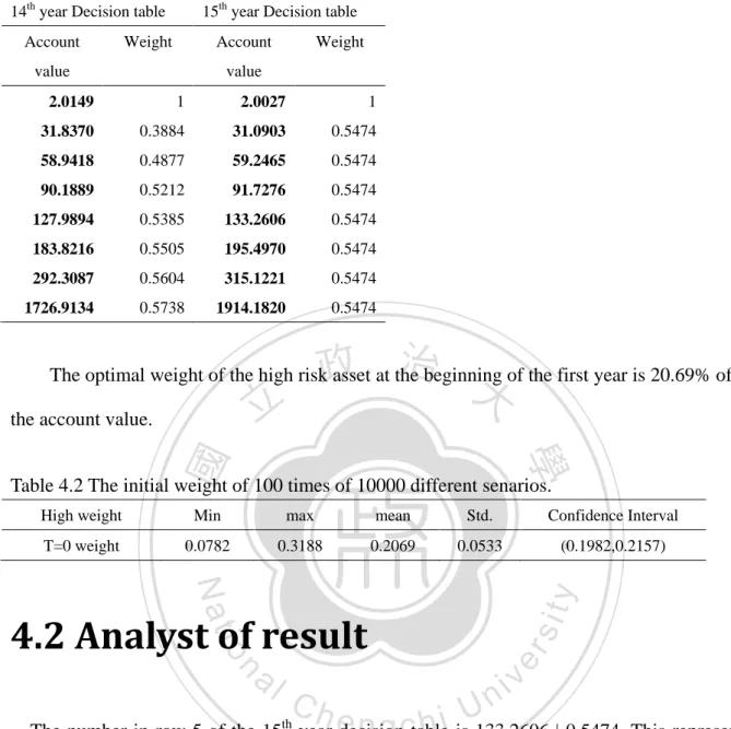
(28) 101.5925. 0.1747. 101.1722. 0.2012. 99.8556. 0.2403. 98.5699. 0.2691. 107.0615. 0.1793. 107.2955. 0.2212. 106.9869. 0.2642. 106.1531. 0.2927. 113.1982. 0.1917. 113.9482. 0.2446. 114.1260. 0.2888. 114.1978. 0.3139. 119.7715. 0.2063. 121.2063. 0.2620. 121.8542. 0.3104. 122.8557. 0.3333. 126.5910. 0.2273. 129.2007. 0.2853. 130.4498. 0.3311. 133.0690. 0.3522. 133.9748. 0.2449. 137.9961. 0.3075. 140.4042. 0.3514. 143.9527. 0.3687. 142.8525. 0.2639. 147.9234. 0.3272. 152.2078. 0.3714. 156.9942. 0.3851. 152.7698. 0.2848. 159.5346. 0.3476. 165.8638. 0.3902. 172.4563. 0.4009. 164.9570. 0.3073. 173.7981. 0.3680. 182.5998. 0.4087. 191.5850. 0.4164. 181.3185. 0.3298. 193.5996. 0.3907. 205.0024. 0.4283. 216.9486. 0.4325. 206.0573. 0.3545. 222.4401. 0.4151. 240.6127. 0.4512. 259.7028. 0.4521. 251.4233. 0.3831. 276.7924. 0.4461. 305.7537. 0.4784. 337.1840. 0.4743. 490.9976. 0.4185. 605.5099. 858.4267. 0.5181. 立. 10th year Decision table. Account. ‧ 國. value. Weight. 11th year Decision table. 12th year Decision table. Weight. Account. value. Weight. value. 22.1338. 1. 24.9976. 39.0144. 1. 35.8796. 1. 50.8050. 0.2024. 47.9872. 62.2562. 0.1693. 73.3929. 0.2269. 84.3902. Weight. value 1. 1. 22.8908. 1. 42.2217. 0.1778. 40.5065. 0.2904. 0.1582. 58.2800. 0.3031. 57.2786. 0.3875. 59.3587. 0.2087. 75.0139. 0.3739. 74.6895. 0.4346. 0.2802. 93.7684. 0.2812. a 82.9112l. 95.9582. 0.3240. 95.3614. 108.8657. 0.3585. 108.9543. 0.3893. 123.0092. 0.3862. 125.0274. 140.3800. 0.4114. 160.1840. y. 1. Account. 2.0388. 25.3847. 1. io. sit. 2.0137. er. 1. ‧. 2.0191. 2.0271. Nat. 1. 13th year Decision table. 學. Account. 0.5106 0.5319 693.4651 治 政 大. i v0.4469. 94.8921. 0.4652. 116.8486. 0.4856. 0.4708. 143.5470. 0.5015. 171.6002. 0.4904. 180.8500. 0.5155. 0.4127. 220.7676. 0.5088. 235.5447. 0.5277. 144.5803. 0.4335. 320.6413. 0.5283. 346.2595. 0.5403. 0.4329. 166.3660. 0.4505. 1214.7322. 0.5589. 1473.5948. 0.5603. 186.9743. 0.4542. 196.1231. 0.4672. 230.5280. 0.4775. 244.1569. 0.4853. 313.1269. 0.5032. 339.1812. 0.5055. 939.1228. 0.5493. 1071.3052. 0.5398. n. 71.0390. C h0.3283 113.9005U n 0.3624 e n g c139.2249 hi. 20. 0.4176.
(29) 14th year Decision table Account. 15th year Decision table. Weight. Account. value. Weight. value. 2.0149. 1. 2.0027. 1. 31.8370. 0.3884. 31.0903. 0.5474. 58.9418. 0.4877. 59.2465. 0.5474. 90.1889. 0.5212. 91.7276. 0.5474. 127.9894. 0.5385. 133.2606. 0.5474. 183.8216. 0.5505. 195.4970. 0.5474. 292.3087. 0.5604. 315.1221. 0.5474. 1726.9134. 0.5738. 1914.1820. 0.5474. 政 治 大. The optimal weight of the high risk asset at the beginning of the first year is 20.69% of. 立. the account value.. ‧ 國. 學. Table 4.2 The initial weight of 100 times of 10000 different senarios. High weight. max. mean. Std.. Confidence Interval. 0.0782. 0.3188. 0.2069. 0.0533. ‧. T=0 weight. Min. Nat. sit. y. (0.1982,0.2157). n. al. er. io. 4.2 Analyst of result Ch. th. engchi. i n U. v. The number in row 5 of the 15 year decision table is 133.2606 | 0.5474. This represents that the account value is 133.2606 in the beginning of year 15, and the optimal utility weight of high risk asset is 0.5474; The number in row 10 in the 10th year decision table is 123.0092 | 0.3862. This represents that the account value is 123.0090 in the beginning of year 10, and the optimal utility weight of high risk asset is 0.3862.. In the 15th year decision table, the only circumstances that the weight is 1 is when the account value equals to2.0027 and other weights are 0.5474. The reason is that the account. 21.
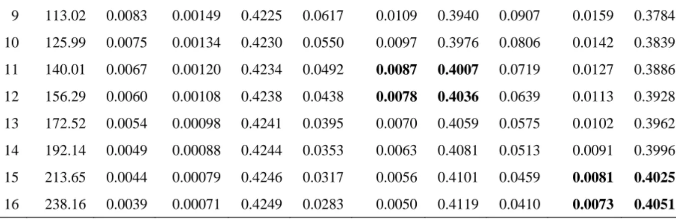
(30) value 2.0027 is very low, and it has very large probability to fall below the guaranteed value (two dollars) in the end of year 15. But even if the account value dropped below 2 dollars, the policyholder can still get guaranteed value. In this guaranteed condition, the policyholder will invest higher proportion in high-risk asset. In other account values of 15th year decision table, the weights of high-risk asset are the same. This is due to the power utility function assumption. In a almost no guaranteed situation, the weight of any account value will be the same.. 政 治 大 as the account value goes up. When the account value becomes smaller, and it could be less 立 In the other year decision tables, the weight of high risk asset goes down first and goes up. ‧ 國. 學. than the guaranteed value in the future. In this situation, the weight of high risk asset will be weighted higher. As the asset value becomes smaller, the weight of high risk asset will close. ‧. to 1. Because the investment account is guaranteed, the policyholder can tolerance asset value. sit. y. Nat. fell below the guaranteed value. However, we cannot find a definite reason to explain the. io. n. al. er. phenomena the weight of high risk asset increases as the asset value increases.. Ch. i n U. v. One of the explanations comes from the fixed withdrawal of the policyholder at the. engchi. beginning of each year. When the account value is low, the ratio of withdraw amount to the account value is big; When the account value is high, the ratio of withdraw to the account value is small. We assume three different withdraw amounts which are equal to 1, 7, and 10, and examine the two period strategy from year 13 to year 15. Table 4.2.1 displays results.. The account values at the beginning of year 14 are assumed to range from 21.47 to 248.16, and the policyholder will withdraw now and one year later. Based on the scenario, we then simulate 10000 scenarios and calculate the account value at the beginning of year 15 and the. 22.
(31) optimal weight of high risk asset. We find that the optimal weight is related to the volatility of the ratio of withdraw to the account value. If volatilities of the ratio of withdraw to the account value among different cases are close, then the corresponding weights are close and similar. When the withdraw amount is equal to 1 and the volatility of the ratio is 0.00809, the weight is 0.4026 (in row 1). This set of values (0.00809, 0.4026) is between row 11 and row 12 when the withdraw amount is 7 and between row 15 and row 16 when the withdraw amount is 10. The volatility of the account asset will become larger when the ratio of withdraw to the account value increases. The ratio:. 立. 政 治 大. ‧ 國. 學. To the policyholder‟s point of view, the volatility of the account value will go up as the. ‧. volatility of the ratio of withdrawal to his own account value goes up. As a result, the. sit. y. Nat. policyholder will put lower proportion on high-risk asset. This can explain why weights of. io. n. al. er. high-risk asset will go up as account values go up in the case of high asset values.. i n U. Table 4.3 The explain of decision table Account value at t=14. Withdraw=1. Ch. Mean. Volatility. weight. of ratio. of ratio. e n gWithdraw=7 chi. v. Withdraw=10. Mean. Volatility. weight. Mean. Volatility. weight. at t=14. of ratio. of ratio. at t=14. of ratio. of ratio. at t=14. 1. 21.47. 0.0457. 0.00809. 0.4026. 0.4568. 0.1129. 0.9999. 0.8233. 0.2034. 0.9999. 2. 34.24. 0.0281. 0.00501. 0.4120. 0.2402. 0.0406. 0.2972. 0.3856. 0.0665. 0.3532. 3. 45.61. 0.0209. 0.00374. 0.4158. 0.1695. 0.0291. 0.3359. 0.2626. 0.0441. 0.2849. 4. 56.18. 0.0169. 0.00303. 0.4179. 0.1330. 0.0231. 0.3556. 0.2024. 0.0345. 0.3179. 5. 66.60. 0.0142. 0.00255. 0.4194. 0.1098. 0.0191. 0.3682. 0.1651. 0.0284. 0.3382. 6. 77.16. 0.0123. 0.00219. 0.4204. 0.0933. 0.0163. 0.3771. 0.1392. 0.0241. 0.3523. 7. 88.72. 0.0107. 0.00191. 0.4213. 0.0801. 0.0141. 0.3841. 0.1187. 0.0207. 0.3633. 8. 101.13. 0.0093. 0.00167. 0.4220. 0.0695. 0.0122. 0.3898. 0.1026. 0.0179. 0.3720. 23.
(32) 9. 113.02. 0.0083. 0.00149. 0.4225. 0.0617. 0.0109. 0.3940. 0.0907. 0.0159. 0.3784. 10. 125.99. 0.0075. 0.00134. 0.4230. 0.0550. 0.0097. 0.3976. 0.0806. 0.0142. 0.3839. 11. 140.01. 0.0067. 0.00120. 0.4234. 0.0492. 0.0087. 0.4007. 0.0719. 0.0127. 0.3886. 12. 156.29. 0.0060. 0.00108. 0.4238. 0.0438. 0.0078. 0.4036. 0.0639. 0.0113. 0.3928. 13. 172.52. 0.0054. 0.00098. 0.4241. 0.0395. 0.0070. 0.4059. 0.0575. 0.0102. 0.3962. 14. 192.14. 0.0049. 0.00088. 0.4244. 0.0353. 0.0063. 0.4081. 0.0513. 0.0091. 0.3996. 15. 213.65. 0.0044. 0.00079. 0.4246. 0.0317. 0.0056. 0.4101. 0.0459. 0.0081. 0.4025. 16. 238.16. 0.0039. 0.00071. 0.4249. 0.0283. 0.0050. 0.4119. 0.0410. 0.0073. 0.4051. In addition, we calculate the guaranteed cost by the decision table. We use the same asset. 政 治 大 10-year bond yield and 30-year bond yield at 2011/1/1. We simulate 10000 scenarios and 立. assumption with our benchmark. The discount rate is 0.0308, which is the interpolation3 of the. ‧. ‧ 國. Nat. Avg. of cost. var. of cost. VaR.90%. 0.2069. 1.2949. 24.1715. 0. CTE70. Prob. Of ruin. 4.3164. 0.0933. io. er. initial Weight. y. Table 4.4 The cost in 10000 different scenarios. sit. listed in Table 4.4. 學. calculate the cost of each scenarios. The average cost is about 1.29 and the other results are. al. n. v i n C h the VA with GMWB, When the insurance companies price e n g c h i U they almost assume that the policyholders put all their money on the high-risk because they can avoid the deficit. However, not all of the policyholders will allocate all their money in risky asset. In this condition, the guaranteed cost will be overestimated, and it is even 383% greater than our benchmark (see table 4.5). We believe that this approach is not reasonable because the policyholders will consider their own utility function and decide the asset allocation.. 3. The interpolation equation : 0.75* yield of 10-year bond in U.S + 0.25*yield of 30-year bond in U.S at 2011/1/1. 24.
(33) In the next section we consider the condition with the policyholder assigns his account to a fixed weight in each period and calculate the guaranteed cost. We assume weights that are equal to our benchmark‟s initial weight and average weight of each period. The result is listed in table 4.5. From this table, we can find that the average cost (1.2949) of our benchmark is much larger than the average cost of fixed weight in 0.2069 (0.9446) and the average cost of fixed weight in 0.3639 (1.1548). According to this result, we conclude that the expected cost of variable annuities with guaranteed minimum withdrawal benefits will increase when the policyholders have the right to choose his own portfolio. However, the insurance companies. 政 治 大. almost assume that the policyholders puts all their money on the high-risk asset when price. 立. the VA with GMWB. As a result, the guaranteed cost will be overestimated and the. ‧ 國. 學. policyholders will be charged unreasonable insurance fee. ‧. Fixed. %diff of. High risk. %diff of. weight. benchmark. weight. benchmark. asset. benchmark. 0.2069. 0. 0.3639. 0.2069. Avg. weight. 0.3639. al 0.2069. Avg. of cost. 1.2949. 0.9446. Var. of cost. 24.1715. 13.6076. VaR90. 0. CTE70 CTE90. n. Initial weight. sit. %diff of. io. Fixed. er. Nat. Benchmark. y. Table 4.5 The comparison between our benchmark and fixed weights. 0.3639 n C h-43.14% U -27.05% 1.1548 engchi. 75.88%. 1. 383.33%. 0. 1. 174.80%. -10.82%. 3.3704. 160.28% 167.94%. iv. -43.70%. 17.6210. -27.10%. 64.7647. 0. 0. 0. 0. 15.5659. 4.3164. 3.1488. -27.05%. 3.8492. -10.82%. 11.2346. 160.28%. 12.9493. 9.4465. -27.05%. 11.5476. -10.82%. 33.7048. 160.28%. -. In order to know the change of the weight as the account value increases in each periods, we depict it in figure 4.1. We observe that the 5th line is higher than other lines, and this result is consistent with intuition because the policyholder for optimal own utility will put more high risk asset when the account value is lower. But what is this reason that the 25th line is higher. 25.
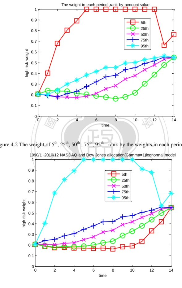
(34) than the 50th,75th and 95th lines in the first few periods and lower than the 50th, 75th and 95th lines after the 6th period? We see the probability of ruin is about 9.33% at the end of the policy in table 4.4. The probability of ruin of 25th line in the periods closed to maturity is very low and the effect of the ratio of withdraw to the account value is big, and therefore the 25th line is lower than other lines except the 95th line. But for the 25th line in the first few periods, the effect of guaranteed is still big because there is still some possibility that the account value touch the guaranteed value. As a result, the twenty-fifty line is higher than the 50th,75th and 95th lines in the first few periods. 政 治 大 The figure 4.2 is the 5 , 25 , median, 75 and 95 lines of the weight of high risk asset in 立 th. th. th. th. ‧ 國. 學. each period in our benchmark. A place worthy of observation is that the 25th line is close to the 5th line in the first few periods, but the 25th line is close to the 50th line in the last few. ‧. periods. This is because the curve of the weight related to the account value is upward, and. sit. y. Nat. the account value of the minimum weight is closed to the expected value in the first few. io. al. n. the last period.. er. period. In contract, the account value of the minimum weight is far from the expected value in. Ch. engchi. 26. i n U. v.
(35) Figure 4.1 The weights of high-risk asset rank by the account value in each period The weight in each period ,rank by account value 1 0.9. 5th 25th 50th 75th 95th. 0.8. high risk weight. 0.7 0.6 0.5 0.4 0.3. 政 治 大. 0.2. 立. 0. 2. 4. 6. 8. 10. time. 學. 0. 12. 14. ‧. ‧ 國. 0.1. Figure 4.2 The weight of 5th, 25th, 50th , 75th, 95th rank by the weights in each period. 0.7. high risk weight. al. n. 0.8. Ch. 0.6. engchi. sit. 5th 25th 50th 75th 95th. er. io. 0.9. y. Nat. 1990/1~2010/12 NASDAQ and Dow Jones allocation(Gamma=1)lognormal model 1. i n U. v. 0.5 0.4 0.3 0.2 0.1 0. 0. 2. 4. 6. 8 time. 27. 10. 12. 14.
(36) 4.3 The improvement of the policyholder’s expected utility In this section, we discuss whether the utility of the policyholder will increase when considering the effect of asset allocation. The results are listed at Table 4.6 and Figure 4.3. The improvement of the policyholder‟s expected utility is about 1.3% compared to the. 政 治 大. expected utility given the weight of high risk asset is fixed in every period.. 立. Table 4.6 The summary of expected utility. 0.2788. 1. 4.1480. 4.2098. 3.9372. 126.0946. 143.8954. 201.4926. n. al. Ch. engchi. 28. y. i n U. v. benchmark. -. sit. io. at t=15. 0. er. Expected withdraw. weight. Nat. Expected utility. High risk asset. ‧. high risk asset. ‧ 國. Fixed weight of. Optimal fixed. 學. Low risk asset. 4.2629 148.5668.
(37) Figure 4.3 The difference of utility between our benchmark and the fixed weight the difference of between our benchmark and the fixed weight 4.35 fixed weight benchmark. 4.3. the expected utility. 4.25 4.2 4.15 4.1 4.05. 立. 4. 0. 0.1. ‧ 國. 3.9. 學. 3.95. 政 治 大. 0.2. 0.8. 0.9. 1. ‧. 0.3 0.4 0.5 0.6 0.7 the weight of hisk risk asset. sit. y. Nat. n. al. er. io. 4.4 The result of VA with GMMB Ch. engchi. i n U. v. We assume a 15-year variable annuities with GMMB, and the single premium is 100 dollars. At the end of the 15th year, the policyholder will be guaranteed that receives the 100 dollars at least. Then other assumptions are the same with our benchmark. The summary of the result is listed in table 4.7. For a policyholder, he will put higher proportion on the high risk asset when he buy the VA with GMMB than GMWB. The reason is that the policyholder doesn‟t consider the volatility generated by the withdraw, and therefore the policyholder is willing to bear more risk.. 29.
(38) Table 4.7 The summary of expected utility Product type. initial Weight. Avg. of cost. var. of cost. VaR.90%. CTE70. Prob. Of ruin. GMWB GMMB. 0.2069 0.8502. 1.2949 2.5731. 24.1715 65.6230. 0 8.0557. 4.3164 8.5772. 0.0933 0.1270. The figure 4.4 shows that the policyholder will put more high risk asset when the account value goes up, and this is because the effect of guaranteed. Figure 4.4 The average weight ranked by the account value in each period of VA with GMMB. 政 治 大. The average weight ranked by the account value in each period of VA with GMMB 1. 立. 0.9. 0.6. sit. io. al. n. 0.3. er. 0.4. y. Nat. 0.5. ‧. ‧ 國. 0.7. high risk weight. 學. 0.8. 0.2. Ch. 0.1 0. 0. 2. 4. engchi. 6. 8 time. 30. i n U 10. v. 12. 5th 25th 50th 75th 95th. 14.
(39) 5 sensitivity analysis In this study, we use stochastic simulation as an approach to find the optimal asset allocation strategy and calculate the expected cost. However, the simulation approach is limited to parameter risks and model risks. It is important to examine the sensitivity of model outputs to each key parameter. In this section, we explore the influence of several parameters on model‟s outputs one at a time. We first investigate the influence of risk-averse parameters;. 政 治 大. are the expected cost the same under different parameters? Second, what is the influence. 立. when one considers the management charge? Finally, in order to know whether there exists. ‧ 國. 學. some asset model error, we assume that asset return processes are subject to ARIMA-GARCH model and compare the asset allocation and expected cost between ARIMA-GARCH model. ‧. and lognormal model.. sit. y. Nat. n. al. Ch. engchi risk-averse parameter. the er. io. 5.1 Sensitivity analysis of. i n U. v. In this section, we set different relative risk-averse parameters of the policyholder, and compare costs among different risk-averse parameters. In the table 5.1, we can find that all of the numbers related the guaranteed cost will increase when the policyholder who is more aggressive on risk will choose more weight of risky asset. In other word, the insurance companies will have more responsibility for holding reserve.. 31.
(40) Table 5.1 The summary of different risk-averse parameter in 10000 scenarios Gamma. Initial. Average. Average. Variance of. Weight. weight. cost. cost. VaR90. CTE70. prob. of ruin. 0.5. 0.9087. 0.8435. 2.9293. 58.2773. 13.6649. 9.7644. 0.1779. 0.75. 0.3762. 0.5381. 1.6874. 33.2665. 3.0507. 5.6247. 0.1120. 1. 0.2069. 0.3642. 1.2949. 24.1715. 0.0000. 4.3164. 0.0933. 2. 0.0893. 0.1494. 1.0123. 17.7468. 0.0000. 3.3745. 0.0825. Then we compare expected costs among different risk-averse parameters with the cost of related fixed weight. First, we compare average cost among different risk-averse parameters. 政 治 大. with the cost of related fixed initial weight, and find that the differences between these two. 立. cost have no regular pattern. The percent difference given the gamma is equal to 0.5 is 0.8%,. ‧ 國. 學. but the percent difference given the gamma is equal to 0.75 is 43.51%. It has big difference between the two percent difference. Therefore we compare the cost again with the cost of. ‧. related fixed average weight, and find that all of the percent differences between the two cost. er. io. sit. y. Nat. are about 12%.. Table 5.2 The difference cost between variable weight and fixed initial and average weights. al. n. Gamma. Initial. Average. Weight. cost(A). Ch. The cost of. % diff. e n g c(A-B)/B hi. fixed initial. iv Average n U weight. weight(B). The cost of. % diff. fixed average. (A-C)/C. weight(C). 0.5. 0.9087. 2.9293. 2.9061. 0.80%. 0.8435. 2.6033. 12.52%. 0.75. 0.3762. 1.6874. 1.1758. 43.51%. 0.5381. 1.5230. 10.79%. 1. 0.2069. 1.2949. 0.9446. 37.08%. 0.3642. 1.1553. 12.08%. 2. 0.0893. 1.0123. 0.8649. 17.04%. 0.1494. 0.8971. 12.84%. After this, we calculate the differences of the variance of cost and CTE70 between variable weight and fixed average weight, and find that the CTE70 has the same result with expected. 32.
(41) cost and the variance of cost will increase as the parameter of risk-averse increases. The result of CTE70 is due to the probabilities of ruin are less than 30%, and the percent differences are the same as the expected cost certainly. Table 5.3 The other difference between variable weight and fixed initial and average weight Gamma. Variance of. Fixed average. cost. % diff.. CTE70. Fixed average. weight. % diff.. weight. 0.5. 58.2773. 47.5744. 22.50%. 9.7644. 8.6776. 12.52%. 0.75. 33.2665. 25.0336. 32.89%. 5.6247. 5.0765. 10.80%. 1. 24.1715. 17.6310. 37.10%. 4.3164. 3.8508. 12.09%. 2. 17.7468. 12.7011. 39.73% 3.3745 政 治 大. 2.9901. 12.85%. 立. Figure 5.1 The expected cost in different utility parameter compared to fixed initial weight. ‧ 國. sit. n. al. er. io. 2. y. Nat. 2.5. expected cost. fixed weight gamma=0.5 gamma=0.75 gamma=1 gamma=2. ‧. 3. 學. the average of cost with fixed inital weight in different utility parameter. 3.5. 1.5. Ch. engchi. i n U. v. 1. 0.5. 0. 0.1. 0.2. 0.3. 0.4 0.5 0.6 high risk asset weight. 33. 0.7. 0.8. 0.9. 1.
(42) Figure 5.2 The expected cost in different utility parameter compared to fixed average weight the average of cost with fixed averaged weight in different utility parameter 3.5 fixed weight gamma=0.5 gamma=0.75 gamma=1 gamma=2. 3. expected cost. 2.5. 2. 1.5. 政 治 大. 1. 立 0.1. 0.2. 0.3. 0.4 0.5 0.6 high risk asset weight. 0.7. 0.8. 學. 0. ‧ 國. 0.5. 0.9. 1. Figure 5.3 The average weight at each time given different utility parameter. ‧. 0.8. gamma=0.5 gamma=0.75 gamma=1 gamma=2. 0.7. average weight. sit. n. al. er. io. 0.9. y. Nat. average weight at each time given different utility parameter 1. 0.6. Ch. engchi. i n U. v. 0.5 0.4 0.3 0.2 0.1 0. 0. 2. 4. 6. 8 time. 34. 10. 12. 14.
(43) The figure 5.3 shows that the average weights in each period given different utility parameters. Given the utility parameter is equal to 0.5, the average weight will decrease when the time closes to maturity. It meets the life cycle allocation; which represent the policyholder will put his own asset on high risk asset when close to maturity. However, in the other hand, the average weight will increase when the time closes to maturity given the utility parameters are equal to or greater than 0.75. This is due to the influence of withdraw; the policyholder will receive more times of future withdraw in the first few periods, so the policyholder will have more investment risk and put less money on high risk asset which we mention before.. 政 治 大 5.2 sensitivity立analysis of model. ‧ 國. 學 ‧. In order to explore whether our approach in different asset model will have similar results, we compare the difference between lognormal model and ARIMA-GARCH model-.. y. Nat. n. al. er. io. sit. The result is listed in Table 5.4.. v. Table 5.4 (The difference of the cost of GMWB between lognormal model and ARIMA-GARCH model) Gamma(risk-averse. Gamma. parameter). Ch. Weighted in high risk. i n U. i eExpected n g c hVariance cost. of cost. VaR 90%. CTE70%. Ruin probability. (t=0). Lognormal. 0.5. 0.9087. 2.9293. 58.2773. 13.6649. 9.7644. 0.1779. ARIMA-GARCH. 0.5. 0.6902. 5.8229. 195.9438. 28.6194. 19.4097. 0.1960. -24.05%. 98.78%. 236.23%. 109.44%. 98.78%. 10.17%. Percentage change. Lognormal. 0.75. 0.3762. 1.6874. 33.2665. 3.0507. 5.6247. 0.1120. ARIMA-GARCH. 0.75. 0.1279. 2.2134. 69.8356. 0.0000. 7.3782. 0.0945. -66.00%. 31.18%. 109.93%. -100.00%. 31.17%. -15.63%. Percentage change. 35.
(44) Lognormal. 1. 0.2069. 1.2949. 24.1715. 0.0000. 4.3164. 0.0933. ARIMA-GARCH. 1. 0.0358. 1.6295. 49.1840. 0.0000. 5.4317. 0.0754. -82.70%. 25.84%. 103.48%. -. 25.84%. -19.19%. Percentage change. Lognormal. 2. 0.0893. 1.0123. 17.7468. 0.0000. 3.3745. 0.0825. ARIMA-GARCH. 2. 0.0100. 1.3179. 36.3768. 0.0000. 4.3931. 0.0710. -88.80%. 30.19%. 104.98%. -. 30.19%. -13.94%. Percentage change. We can find that the expected cost in ARIMA-GARCH model is greater than the expected. 政 治 大 than lognormal model. When the market goes down, the insurance company needs to pay 立. cost in lognormal model. This is because that the ARIMA-GARCH model is more fat-tailed. ‧ 國. 學. more guaranteed costs in ARIMA-GARCH model.. Table 5.5 The difference of expected cost between different asset models. 30.19%. 2.9293 5.8229. 3.3704 10.3051. 98.78%. 205.75%. sit. 1.6874 2.2134. high risk asset. er. 1.2949 1.6295. y. Benchmark Gamma=0.75 Gamma=0.5 (Gamma=1). n. al. ‧. 1.0123 1.3179. io. Lognormal 0.8503 ARIMA0.9755 GARCH Percentage 14.71% change. Gamma=2. Nat. Low risk asset. Ch. 25.84%. engchi. 36. i n U. 31.18%. v.
(45) 6 Conclusion The main goal of this study is to explore whether the guaranteed cost will increase when the policyholders have the right to rebalance his own account in every period. We can get the following conclusions. First, The guaranteed cost of variable annuities with GMWB when the policyholder can rebalance his own asset allocation in every year is about 12% more than the guaranteed cost of the fixed weight which is calculated by the average of the weights in each year of our optimal allocation. Second, the optimal allocation is affected by the asset model and the risk averse attitude of the policyholder in our model. When the asset model is a fat-. 政 治 大 more guaranteed cost the insurance companies need to afford . 立. tailed model, it needs more guaranteed cost; when the policyholder is more aggressive, the. ‧ 國. 學. In our study, there are still several restrictions when we price the guaranteed products. First, The main restriction in our study is that we assume that the policyholder will hold the. ‧. policy until the end of the policy, and the policyholder doesn‟t have the right to terminate the policy in any time in the light of actual conditions. However, it will be involved in the issues. y. Nat. sit. of the inter-temporal utility and the discount of utility, and the issue is not in our study.. al. er. io. Second, we use backward method to decide the optimal allocation of the policyholder.. n. However, if we want to price products such as VA with GMAB, it does not work. The reason. Ch. i n U. v. is that we don‟t know the renew guaranteed value at the last period, and there is no enough. engchi. information to calculate the optimal allocation.. The future studies may have the following issues. First, we assume there are only two linked assets in our study, but the dynamic programming method can apply to three assets, four assets, or even more. The future studies can attempt more linked assets. Second, we propose the risk-free interest are fixed, but the risk-free interest rate model can transfer to stochastic interest rate model, and the future research can consider the withdrawal behavior of the policyholder. Furthermore, there are many different utility functions such as exponential utility function and logarithm utility function in financial economic theory, and the different utility functions may generate different results in our method. As a result, the sensitivity. 37.
(46) analyst can compare the different utility functions.. 立. 政 治 大. ‧. ‧ 國. 學. n. er. io. sit. y. Nat. al. Ch. engchi. 38. i n U. v.
(47) Reference. 5. 6.. Brennan, M.J., and Schwartz, E.S., 1976. The Pricing of Equity-linked Life Insurance Policies with an Asset Value Guarantee. Journal of Financial Economics 3 (1), 195–213. Brennan, M.J. and Schwartz, E.S., 1979, Alternative Investment Strategies for the Issuers of Equity-linked Life Insurance Policies with an Asset Value Guarantee, Journal of Business 52, 63-93. Coleman, T.F. ,Kim, Y., and Patron, M. (2005), Hedging Guaranteed Variable Annuities Under Both Equity and Interest Rate Risks, Cornell University, New York. Coleman, T.F. ,Kim, Y., and Patron, M. (2005), Robustly Hedging Variable Annuities With Guaranteed Under Jump and Volatility Risk, The Journal of Risk and Insurance, 2007, Vol. 74, No,2, 347-376. Chen, K. Verzal, and P. Forsyth. The effect of modeling parameters on the value of GMWB guarantees. Insurance: Mathematics and Economics, 43(1):165-173, 2008 Delbaen, F., and M. Yor, 2002, Passport Options, Mathematical Finance, 12(4): 299-328. Hardy, M.R. 2000, Hedging and Reserving for Single-premium Segregated Fund Contracts. North American Actuarial Journal 4 (2), 63-74.. Nat. 9.. ‧. 8.. 學. 7.. 立. 政 治 大. y. 4.. io. sit. 3.. n. al. er. 2.. Aase, K.K., and Persson, S.A., 1994, Pricing of Unit-linked Life Insurance Policies. Scandinavian Actuarial Journal 1, 26-52. Aase, K.K., and Persson, S.A., 1997, Valuation of the Minimum Guaranteed Return Embedded in Life Insurance Contracts. Journal of Risk and Insurance 64 (4), 599-617. Bacinello, A. R., Biffis, E., and Millossovich, P., 2009, Regression-Based Algorithm for Life Insurance Contracts with Surrender Guarantees, to appear in Quantitative Finance, Version as of April 7, 2009. Boyle, P.P., Schwartz, E., 1977. Equilibrium Prices of Guarantees under Equity-linked Contracts. Journal of Risk and Insurance 44(2), 639–680. Boyle, P.P. and Schwartz, E.S., 1997, Equilibrium Prices of Guarantees under Equity-linked Contracts. Journal of Risk and Insurance 44, 639-680. Boyle, P.P. and Hardy, M.R., 1997, Reserving for Maturity Guarantees: Two Approaches. Insurance: Mathematics and Economics 21, 113-127. Boyle, P.P. and Hardy, M.R. 2003, Guaranteed Annuity Options. Astin Bulletin 33 (2), 125-152. ‧ 國. 1.. 10. 11.. 12. 13. 14.. Ch. engchi. i n U. v. 15. Hardy, M.R., 2003, Investment Guarantees: Modeling and Risk Management for Equity-linked Life Insurance. 1st ed., Hoboken, N.J.: Wiley.. 39.
(48) 16. Holz, D., Kling, A., and Ru, J. , 2007, GMWB For Life An Analysis of Lifetime Withdrawal Guarantees. Working Paper, Ulm University, 2007. 17. Hung,D.Y.,2009,The numerical solution of optimal asset allocation dynamic. 22.. 學. 23.. 立. 政 治 大. ‧. Nat. y. 21.. io. sit. 20.. n. al. er. 19.. ‧ 國. 18.. programming. Cheng-Chi University master degree paper. Liu,Y,2006, 2010Pricing and Hedging the Guaranteed Minimum Withdrawal Benefits in Variable Annuities. Working Paper. Milevsky, M.A., and Posner, S.E., 2001, The Titanic option: Valuation of Guaranteed Minimum DEATH Benefit in Variable Annuities and Mutual Fund. The Journal of Risk and Insurance, Vol. 68, No. 1,91-216,2001. Milevsky, M.A., Salisbury, T.S., 2006. Financial Valuation of Guaranteed Minimum Withdrawal Benefits. Insurance: Mathematics and Economics 38, 21-38 Nielsen, J.A., K. Sandmann, 1995, Equity-Linked Life Insurance: a Model with Stochastic Interest Rates. Insurances: Mathematics and Economics, 16,225-253. Turnbull. Understanding the true cost of VA hedging in volatile markets. Technical report, Nov 2008. J. Peng, K. Leung, and Y. Kwong. Pricing Guaranteed Minimal Withdrawal Benefit under the stochastic interest rate. Technical report, Jan 2009.. Ch. engchi. 40. i n U. v.
(49) Appendix A. The data of the main five indexes in U.S. Table Appendix A.1 The normal test of main five indexes in U.S ( Expire at 2010/12) P value. S&P500. P value. P value. Dow Jones. P value. NASDAQ. S&P100. P value. 0.0322. 18.42. 0.0025. 4.85. 0.4341. 6.90. 0.2281*. 24.08. 0.0002. 2000/1~. 10.96. 0.0521. 16.15. 0.0064. 4.90. 0.4277*. 7.49. 0.1865*. 19.80. 0.0014. 1999/1~. 11.58. 0.0410. 11.05. 0.0503**. 3.17. 0.6745*. 0.2401*. 15.26. 0.0093. 1998/1~. 11.61. 0.0406. 12.52. 0.0283. 5.03. 0.4121*. 4.60. 0.4670*. 16.43. 0.0057. 1997/1~. 10.94. 0.0527**. 12.19. 0.0323. 6.48. 0.2625*. 4.96. 0.4205*. 14.30. 0.0138. 1996/1~. 12.07. 0.0339. 立. 政 治 大. 6.75. 14.93. 0.0107. 6.97. 0.2230*. 5.43. 0.3657*. 14.27. 0.0140. 1995/1~. 14.69. 0.0118. 14.06. 0.0152. 6.29. 0.2787*. 9.23. 17.25. 0.0041. 1994/1~. 12.34. 0.0304. 16.47. 0.0056. 5.93. 0.3133*. 學. 0.1003*. 9.16. 0.1029*. 16.46. 0.0056. 1993/1~. 14.78. 0.0113. 18.80. 0.0021. 7.18. 0.2077*. 12.17. 0.0325. 15.32. 0.0091. 1992/1~. 17.77. 0.0033. 19.20. 0.0018. 8.22. 0.1446*. 12.65. 0.0269. 13.35. 0.0203. 1991/1~. 15.55. 0.0082. 18.01. 0.0029. 8.94. 0.1114*. 12.85. 0.0248. 12.11. 0.0334. 1990/1~. 16.93. 0.0046. 16.12. 0.0065. 9.74. 0.0829**. 10.17. 0.0706**. 12.22. 0.0319. 1989/1~. 16.63. 0.0053. 18.74. 0.0021. 9.51. 0.0902**. 11.21. 0.0474. 12.98. 0.0236. 1988/1~. 16.28. 0.0061. al. 0.0021. 8.49. 0.1313*. 0.0359. 11.91. 0.0360. n. Ch. y. sit er. io. 18.76. ‧. 12.20. Nat. 2001/1~. ‧ 國. Russell 2000. n U engchi. 11.92. iv. Table Appendix A.2 Annualized return and volatility of five main indexes on monthly information 1990/1~2010/12. Annualized return Annualized volatility. Russell 2000. S&P500. Dow Jones Industrial Average. 0.0845. 0.0659. 0.0735. 0.0937. 0.0634. 0.1962. 0.1519. 0.1496. 0.2429. 0.1548. (Source: YAHOO! In U.S). 41. NASDAQ Composite. S&P100.
(50) Table Appendix A.3 Correlation table of five main indexes on monthly information Russell 2000. Dow Jones Industrial. S&P500. NASDAQ. Average Russell 2000 S&P500 Dow Jones Industrial Average NASDAQ Composite S&P100. S&P100. Composite. 1 0.8009. 0.8009 1. 0.7188 0.9416. 0.8554 0.828. 0.7534 0.9862. 0.7188. 0.9416. 1. 0.7064. 0.9427. 0.8554. 0.828. 0.7064. 1. 0.8292. 0.7534. 0.9862. 0.9427. 0.8292. 1. (Source: YAHOO! In U.S). 立. 政 治 大. Table Appendix A.4 The order of ARIMA in NASDAQ index. 1. 1. 1. 2. 1. 2. 0. 0.000616. -3.393443. 431.4025. 1. 0.000653. -3.425473. -3.397461. 433.6096. 1. 0.013978. -3.427027. -3.384890. 433.0919. 2. 0.015278. -3.417477. -3.394800. 1. 0.014014. -3.419096. 0.014854. -3.409046. 2. n. al. y. 1. AIC. 431.1846. sit. 1. R-square. -3.396486. 433.0965. -3.380701. 431.1308. SBIC. LR. er. 0. -3.421534. ‧ 國. 1. LR. ‧. 1. q. 學. 1. SBIC. io. p. Nat. c. i n C Table Appendix A.5 The order of ARIMA Jonesi index U h einnDoe h c g c p q R-square AIC. v. 1. 1. 0. 0.014735. -2.471756. -2.460451. 312.2053. 1. 0. 1. 0.014858. -2.475704. -2.447692. 313.9387. 1. 1. 1. 0.014825. -2.463879. -2.421742. 312.2168. 1. 1. 2. 0.014877. -2.455964. -2.399782. 312.2235. 1. 2. 1. 0.078479. -2.518772. -2.462429. 318.8465. 1. 2. 2. 0.071195. -2.502898. -2.432469. 317.8623. 42.
(51) Appendix B. The decision table of GMMB At the section 4.4, we show the result of VA with GMMB, and the below table is the decision table of GMMB.. Weight. Account. 立. value. 25.8205. 0.9825. 78.4719. 0.9974. 72.2897. 89.7860. 0.9568. 89.0365. 0.9814. 95.2350. 0.9232. 96.8972. 99.8978. 0.8928. 103.7390. 104.3687. 0.8649. 108.8753. 0.8412. 113.7488. 0.8144. 124.6159. 119.4148. 0.7890. 133.4243. 126.7116. 0.7562. 145.1522. 138.4424. 0.7222. 164.4849. 242.1262. 0.5913. 367.8705. 1. 71.4009. 1. 83.6502. 1. 84.3455. 1. 0.9429. 91.8640. 0.9930. 93.9610. 0.9937. 0.9072. 98.8640. 0.9707. 102.1964. 0.9746. 110.2776. 0.8655. 105.3292. 0.9356. 109.9459. 0.9378. 117.0591. 0.8287. 111.5283. 0.9028. 117.3902. 0.8884. 0.7887. 117.8442. 0.8637. 125.0781. 0.8373. 133.0205. 0.7919. 141.5099. 0.7509. 151.1070. 0.7158. n. 0.8274 v i n C h0.7143 131.3956 U 0.7934 e n g 139.1076 chi 0.6638 0.7542 0.7514. Weight. Account. 124.4178. 0.5657. 7th year Decision table. value 18.4201. 1. Nat. 6th year Decision table Account. 20.2163. al. 16.5853. 148.2108. 0.7288. 162.5776. 0.6882. 159.5394. 0.6979. 177.0545. 0.6536. 175.4649. 0.6674. 197.2879. 0.6194. 202.8585. 0.6255. 233.9415. 0.5909. 501.1539. 0.5698. 653.2512. 0.5544. 8th year Decision table. Weight. Account. value 1. 1. ‧. 1. ‧ 國. 82.0379. 30.7111. Weight. value. 學. 1. Account. io. 42.3826. 5th year Decision table. y. value. 4th year Decision table. sit. Account. 治 Weight 政 Account Weight 大 value. 3rd year Decision table. er. 2nd year Decision table. 9th year Decision table. Weight. Account. value 1. 16.3651. 43. Weight. value 1. 13.1072. 1.
(52) 1. 63.0372. 1. 62.5027. 1. 62.7949. 1. 75.6651. 1. 76.3299. 1. 77.1439. 1. 78.3630. 1. 84.6213. 1. 86.2575. 1. 87.9106. 1. 90.0937. 1. 92.1094. 0.9994. 94.5996. 1. 97.1886. 1. 100.1537. 1. 98.8190. 0.9964. 102.0676. 0.9971. 105.4672. 1. 109.3739. 0.9994. 105.0113. 0.9862. 109.0165. 0.9900. 113.2491. 0.9997. 118.2201. 0.9916. 110.9620. 0.9594. 115.6604. 0.9781. 120.8728. 0.9832. 126.6335. 0.9642. 116.7214. 0.9300. 122.2629. 0.9504. 128.3732. 0.9529. 135.0334. 0.9102. 122.5025. 0.8951. 129.0653. 0.9048. 135.9402. 0.9068. 143.5446. 0.8392. 128.3390. 0.8564. 135.8147. 0.8587. 143.6636. 0.8566. 152.2427. 0.7829. 134.2484. 0.8235. 142.6894. 0.8178. 151.4669. 0.8081. 161.0882. 0.7382. 140.3847. 0.7847. 149.8818. 0.7775. 159.8543. 0.7653. 0.6985. 146.8360. 0.7563. 157.5107. 180.4739. 0.6670. 153.7039. 0.7342. 165.7620. 0.7401 168.7438 0.7249 治 政 0.7101 178.3536 大 0.6947. 170.5872. 191.4300. 0.6368. 161.2835. 0.7119. 174.8710. 0.6838. 188.9058. 0.6703. 203.7048. 0.6155. 169.6727. 0.6860. 184.8237. 0.6601. 200.6492. 0.6499. 217.3511. 0.5974. 179.3382. 0.6621. 196.3120. 0.6416. 214.1369. 0.6278. 233.1626. 0.5805. 190.6550. 0.6428. 209.8943. 0.6191. 229.9791. 0.6108. 251.8587. 0.5696. 204.5037. 0.6203. 226.6311. 0.6031. 250.1702. 0.5979. 275.3404. 222.7196. 0.6040. 248.8497. 0.5884. 277.1045. ‧. 0.5596. 0.5885. 306.7487. 0.5523. 248.6439. 0.5877. 281.3096. 0.5783. 316.4414. 0.5788. y. 354.7241. 0.5470. 298.7948. 0.5730. 342.7591. 0.5667. 393.5771. 0.5740. 445.6414. 0.5457. 858.8344. 0.5604. 1093.5610. 0.5608. 1362.4171. er. 1631.8749. 0.5441. io. n. al. Ch. Account. value. 0.5716. n U engchi. 11th year Decision table. Weight. sit. ‧ 國. Nat. 10th year Decision table Account. 立. 學. 63.5875. iv. 12th year Decision table. Weight. Account. value. 13th year Decision table. Weight. Account. value. Weight. value. 11.9964. 1. 12.1431. 1. 11.0220. 1. 9.7949. 1. 72.7350. 1. 73.8933. 1. 75.1403. 1. 76.3941. 1. 93.3464. 1. 95.9490. 1. 98.6699. 1. 101.9382. 1. 109.8064. 1. 113.7187. 1. 117.9737. 1. 122.8129. 1. 124.7092. 0.9984. 130.0035. 0.9979. 135.7629. 0.9997. 142.3342. 0.9955. 138.9119. 0.9618. 145.9905. 0.9253. 153.2537. 0.8984. 161.3492. 0.8101. 153.3263. 0.8554. 162.0244. 0.7782. 171.1028. 0.7489. 181.0513. 0.6683. 168.4052. 0.7578. 179.1015. 0.6904. 190.0669. 0.6606. 201.9280. 0.6042. 44.
(53) 184.9951. 0.6883. 197.6330. 0.6324. 210.5052. 0.6146. 225.1562. 0.5782. 203.3699. 0.6427. 218.4123. 0.5953. 234.1120. 0.5886. 251.1703. 0.5703. 224.6581. 0.6119. 242.6935. 0.5750. 261.9043. 0.5772. 282.0647. 0.5673. 250.6091. 0.5911. 272.5393. 0.5653. 295.9922. 0.5721. 320.3329. 0.5666. 285.0832. 0.5802. 312.0279. 0.5585. 341.3551. 0.5700. 370.9376. 0.5664. 335.8311. 0.5745. 371.3070. 0.5562. 409.3814. 0.5696. 450.1335. 0.5663. 434.6593. 0.5720. 486.4801. 0.5553. 543.5612. 0.5696. 605.9494. 0.5663. 2105.1230. 0.5713. 2459.2426. 0.5541. 2915.8501. 0.5690. 3573.7358. 0.5659. Account. value. value. Weight. 政1 治 大 1. 8.0945. 77.8515. 1. 79.3659. 105.1295. 1. 108.8841. 1. 127.8087. 1. 133.0541. 1. 148.9906. 0.9655. 156.0086. 0.5824. 169.7268. 0.6756. 178.6510. 0.5502. 191.4258. 0.6027. 202.1420. 0.5475. 214.5025. 0.5823. 227.4812. 0.5474. 240.1117. 0.5774. 255.7465. 0.5474. 269.1236. 0.5766. 288.0422. 0.5474. 303.3431. 0.5765. 0.5474. 346.2646. 0.5764. al 374.8867. 404.3939. 0.5764. 439.8087. 492.8482. 0.5764. 540.4006. 0.5474. 671.3695. 0.5764. 744.8425. 0.5474. 4299.0267. 0.5761. 5457.2780. 0.5474. ‧ 國. 立. Nat. io. n. 326.4945. Ch. 0.5474. engchi. 0.5474. 45. ‧. 1. 學. 9.3568. y. Weight. sit. Account. 15th year Decision table. er. 14th year Decision table. i n U. v.
(54) The figure is the average weight ranked by weight in each period of VA with GMMB. The average weight ranked by weight in each period of VA with GMMB 1 0.9 0.8. 0.6 0.5 0.4 0.3. 立. 0.2. 2. 4. 6. 8. 10. 12. ‧. time. y. Nat. io. sit. 0. n. al. er. 0. 5th 25th 50th 75th 95th. 政 治 大. 學. 0.1. ‧ 國. high risk weight. 0.7. Ch. engchi. 46. i n U. v. 14.
(55)
數據
+7
相關文件
(十四)廠商為押標金保證金暨其他擔保作業辦法第 33 條之 5 或第 33 條之 6
(十三)廠商為押標金保證金暨其他擔保作業辦法第 33 條之 5 或第 33 條之 6
(十四)廠商為押標金保證金暨其他擔保作業辦法第 33 條之 5 或第 33 條之 6
(十四)廠商為押標金保證金暨其他擔保作業辦法第 33 條之 5 或第 33 條之 6
In this paper, we propose a practical numerical method based on the LSM and the truncated SVD to reconstruct the support of the inhomogeneity in the acoustic equation with
In this paper we establish, by using the obtained second-order calculations and the recent results of [23], complete characterizations of full and tilt stability for locally
In this paper we establish, by using the obtained second-order calculations and the recent results of [25], complete characterizations of full and tilt stability for locally
Table 3 Numerical results for Cadzow, FIHT, PGD, DRI and our proposed pMAP on the noisy signal recovery experiment, including iterations (Iter), CPU time in seconds (Time), root of
