Illuminance formation and color difference of mixed-color
light emitting diodes in a rectangular light pipe: an
analytical approach
Chu-Ming Cheng1,* and Jyh-Long Chern1,2
1Department of Photonics, Institute of Electro-Optical Engineering, Microelectronics and Information System Research Center, National Chiao Tung University, Hsinchu, Taiwan, China
2E-mail: [email protected]
*Corresponding author: [email protected]
Received 18 April 2007; revised 13 September 2007; accepted 29 November 2007; posted 29 November 2007 (Doc. ID 82216); published 18 January 2008
We developed an analytical method of illuminance formation for mixed-color LEDs in a rectangular light pipe in order to derive American National Standards Institute (ANSI) light uniformity, ANSI color uniformity, and color difference of light output using photometry, nonimaging, and colorimetry. The analytical results indicate that the distributions of illuminance and color difference vary with different geometric structures of light pipes and the location of the light sources. It was found that both the ANSI light and the ANSI color uniformity on the exit plane of the light pipe are reduced exponentially with the increase in length of the light pipe. It is evident that a length scale L兾A greater than unity assures that the mixed-color LED sources on the entrance plane are uniformly illuminated with acceptable uniform brightness and color on the exit plane of the rectangular light pipe, where L is the length of the light pipe, and A is a constant, which is a geometric parameter for the scale unit of the light pipe’s input face. Furthermore, the ANSI light uniformity can be minimized, and the ANSI color uniformity can be maximized under the condition of multilight-source locations P⫽ Q ⫽ ⫾A兾4, where P and Q are the coordinates along the long axis and the short axis, respectively, with one being the entrance plane of the light pipe. We can conclude that the optimum form factor of the light pipe is a square shaped cross section, with the length scale L兾A being equal to unity and with multilight sources located individually on positions of A兾4 in order to achieve very uniform illuminations with the highest light efficiency and compact package for the optical system with mixed-color LEDs, where L is the length of the light pipe. © 2008 Optical Society of America
OCIS codes: 120.5240, 220.2740, 230.3670, 230.7370, 330.1730.
1. Introduction
Today’s light emitting diode (LED) technology is widely applied in vehicles, architecture, signal light-ing, backlightlight-ing, and in projection microdisplays [1]. Most of these applications require the shaping of a uniform beam illuminance profile, managing color quality, and saving power consumption while main-taining high luminous efficiency in the illumination systems. There are two kinds of approaches to gen-erate white light with LEDs. One is the phosphor-converted white LED, which provides a compact
integrated package but has a relatively lower lumi-nous efficiency. The other is the mixed-color LED, which provides more light throughput compared to a single phosphor-converted white LED with the same operating power. In practice, however, there are sev-eral technical challenges to creating a mixed-color LED, such as white light homogenizing with the ac-ceptably lowest spatial variation, color mixing, and color balancing with acceptably lowest chromatic variation.
Rectangular light pipes are commonly optical de-vices that manage light properties in illumination systems, especially where extremely uniform illumi-nations with specific illuminance distributions are required [2]. Typical applications are the
illumina-0003-6935/08/030431-11$15.00/0 © 2008 Optical Society of America
tions in the projection display [3], lithography [4], endoscopes [5], and in optical waveguides [6]. A rect-angular light pipe is made with parallel reflective sides with a square or rectangular cross section. The light source can be located on one end of the light pipe, and the other end is then the uniformly illu-minated plane [7]. The shape of the light pipe can modify the original characteristics of the spatial tribution of the light source but not the angular dis-tribution. The uniform illumination on the exit end of the light pipe is determined by the ratio of the length to the cross-sectional dimension of the light pipe [8].
In the literature, the mention of the properties of light pipes is mostly concentrated on transmittance, flux analysis, and irradiance formation for the single light source. Although Derlofske and Hough devel-oped a flux confinement diagram model to discuss the flux propagation of square light pipes and angular distribution [9], and Cheng and Chern developed a semianalytical method to investigate the formation of irradiance distribution [8], to the best of our knowl-edge few papers have investigated the formation of illuminance and the color differences in mixed-color light sources. An earlier investigation of the use of mixed-color LEDs in a light pipe was done by Zhao et al., and it comprised two parts: a computer simulation using a commercial ray tracing soft-ware package with a Monte Carlo algorithm; and an experimental study verifying the results obtained from the simulation [10]. In this paper we developed an analytical method of illuminance formation and color difference for mixing colored LEDs in a rectan-gular light pipe using the methods of photometry [11], nonimaging optics [2], and colorimetry [12]. The different illuminance formations and color differ-ences studied in this paper are the types in which American National Standards Institute (ANSI) light uniformity [13] and ANSI color uniformity [13] vary with the different geometric structures of light pipes. For the purpose of comparison, this paper also in-cludes the formation of illuminance distribution for a single LED source using the same analytical method. There are two kinds of light pipes in terms of ma-terial properties: the hollow light pipe and the solid light pipe. A hollow light pipe is made with parallel mirrors where the sidewalls join together and coatings have a reflectivity of less than 100, and are angular兾 color dependent. A solid light pipe is made of a dielec-tric material with the addition of refraction, Fresnel loss, material absorption, and total internal reflec-tion. Additionally, such a dielectric-filled light pipe brings an index factor through Snell’s law into the treatment of the angular profile and requires a longer length to obtain a given uniformity [2]. To obtain a convenient form of the illuminance formation, we em-ployed the hollow straight light pipe with a perfect reflectivity of 100% for the calculations in this paper. In reality, the finite absorption loss is inevitable. With more times of reflection, the flux of the ray will decrease, which can affect the illuminance distribu-tion. This influence has been explored by Cheng and Chern [8]. For a common coating with a reflectivity of
90%, the difference of the uniformity deviation from that of 100% reflectivity is less than 1% at the length scale L兾A equal and greater than unity, where L is the length of the light pipe, and A is a constant, which is a geometric parameter for the scale unit of the light pipe’s input face. To have a best approximation for the analytical evaluation, we make another assump-tion that the LED is a point light source with Lam-bertian characteristics. In most applications this means that the dimension of the LED source should be much less than the cross-sectional dimension of the light pipe. The considerations of a hollow straight light pipe with a perfect reflectivity and a point light source may limit this study, but it will provide an analytical base for the connection between nonimag-ing and colornonimag-ing to obtain a “uniform” source for illu-mination applications.
The remainder of this paper is organized as follows. In Section 2, we describe the configuration of the light-pipe illumination system. In Section 3, we de-rive the function of illumination formation. In Section 4, we derive the function of color difference. In Sec-tion 5, we investigate the analytical result. Finally, we draw our conclusions in Section 6.
2. Configuration of the Light-Pipe Illumination System
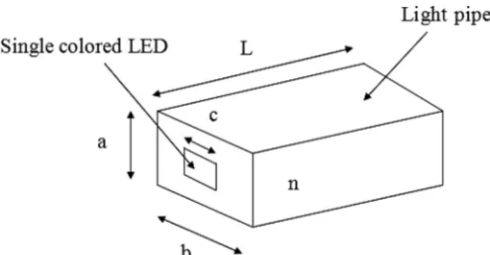
A schematic of an optical system using a rectangular light pipe is shown in Fig. 1. The optical system con-sists of an LED light source with Lambertian angular distribution and a rectangular light pipe, where a and b are the width and the height of the cross section of the light pipe, respectively, L is the length of the light pipe, c is the size of the square light source, and
n is the optical index of the light pipe’s material. The
LED light source is located at the entrance of the light pipe, and the light source has an angular dis-tribution extending from ⫹90° to ⫺90°. The exit is uniformly illuminated by the multiple reflections throughout the light pipe.
The light pipe is made with parallel reflective sides with a rectangular cross section. The virtual image of the light at the entrance of the light pipe has the checkerboard-array-shaped light distribution, which results from the multiple reflections of the light source through the pipe as shown in Fig. 2 [14]. The spaces between each adjacent light spot are: a on the
Fig. 1. Schematic and dimension of the light pipe and the single LED light source.
vertical axis and b on the horizontal axis, which are equal to the width and height of the cross section of the light pipe, respectively, and the size of each light spot is equal to that of the light source. The radiant intensity of each light spot is denoted as Ji,j⬘ as shown
in Fig. 2(b) [14]. The subscripts m and n stand for the reflective times on the horizontal axis and vertical axis, respectively, and the plus and minus values of
i and j denote the opposite directions of the light
source. For example, J1,2⬘ means that the luminous flux of the light spot is reflected one time on the horizontal axis and two times on the vertical axis, and its location is shown in Fig. 2(b).
The schematic of one specific light pipe optical sys-tem with mixed-color LEDs is illustrated in Fig. 3(a). The optical system consists of four colored LED light sources, including one red-colored LED, two green-colored LEDs, and one blue-green-colored LED, and a rect-angular light pipe, where a and b are the width and the height of the cross section of the light pipe, re-spectively, where L is the length of the light pipe, c is the side of the square light source, and n is the optical index of the light-pipe material. The light sources are located at the entrance of the light pipe as shown in Fig. 3(b), where the red LED is located at the coordi-nate共P, ⫺Q兲, the first green LED is located at 共P, Q兲, the second green LED is located at共⫺P, ⫺Q兲, and the blue LED is located at共⫺P, Q兲, respectively, assum-ing that the coordinate of the center for the entrance of the light pipe is共0, 0兲.
3. Functions of Illuminance Formation
The equation of the luminous intensity of the light source with Lambertian characteristics is given as
J⍀⫽ J共兲 ⫽ J0cos, ⫺90° ⱕ ⱕ 90°, (1) where J⍀ is the luminous intensity 共lm sr⫺1兲 of a small incremental area of the source in a direction at an angle from normal to the surface and J0is the luminous intensity of the incremental area in the direction of normal. Thus, we can derive the illumi-nance distribution radiated from the Lambertian light source (i.e., LED) on the exit plane of the light pipe.
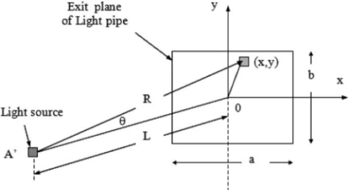
With reference to Fig. 4, we assume that the illu-minance position on the end plane of the light pipe is 共x, y兲, length R is the distance from the light source to
Fig. 2. (a) Principle of the operation of a light pipe. (b) Virtual image at the entrance of the light pipe. The light pipe is made with parallel reflective sides with a rectangular cross section. The mul-tiple reflections of the light source through the pipe can produce a spatial checkerboard-array-shaped light distribution.
Fig. 3. (a) Schematic and dimension of the light pipe. (b) Loca-tions of red, green, and blue LED light sources, i.e., mixed-color LEDs, on the entrance of the light pipe.
the incremental area, length L is the distance from the light source to the end plane of the light pipe, and angle is the angle from normal to the incremental area. The angle can be substituted by L, x, y, and R, and is given by
cos ⫽ L
冑
L2⫹共
x2⫹ y2兲
⫽L
R. (2)
The illuminance distribution on the end plane of the light pipe is a function of cos3, which can be ex-pressed as a function of J0, L, x, and y according to Eqs. (1) and (2) as given by
H共x, y兲 ⫽ J共兲cos
3
L2 ⫽ J0⫻
L2
共
L2⫹ x2⫹ y2兲
2. (3) Then, we determine the individual contribution of illuminance by the virtual light spots on the entrance plane of the light pipe. The illuminance H0,0is radi-ated without any reflection through the light pipe⬃x from⫺a兾2 to ⫹a兾2 and ⬃y from ⫺b兾2 and ⫹b兾2, as shown in Fig. 5 and as given byH00共x, y兲⫽ J0⫻ L2
共
L2⫹ x2⫹ y2兲
2, ⫺ a 2 ⱕxⱕ a 2,⫺ b 2 ⱕyⱕ b 2. (4)Where the values a and b are the width and the height of the cross section of the light pipe, respec-tively. Also, we can derive the illuminances H⬘1,0and
H⬘2,0that are radiated with one time reflection and a two times reflection, respectively, through the light pipe along the⫹x axis direction, as shown in Fig. 5. They are given by
H⬘10共x, y兲⫽ J0⫻ L2 共L2⫹ x2⫹ y2兲2, a 2 ⱕxⱕ 3a 2,⫺ b 2 ⱕyⱕ b 2, (5) H⬘20共x, y兲⫽ J0⫻ 2L2 关L2⫹ x2⫹ y2兴2, 3a 2 ⱕxⱕ 5a 2,⫺ b 2 ⱕyⱕ b 2, (6) where is the reflectivity, and the exponent of is the reflective time. Then, we can derive the practical il-luminance distribution, which is radiated from the individual virtual light spot on the entrance plane of the light pipe, on the exit plane of the light pipe⬃x from ⫺a兾2 to ⫹a兾2 and ⬃y from ⫺b兾2 and ⫹b兾2 using the mirror mapping method according to Eqs. (5) and (6) as given by H10共x, y兲 ⫽ J0⫻ L2
关
L2⫹ 共⫺x ⫹ a兲2⫹ y2兴
2, ⫺a2 ⱕxⱕa 2,⫺ b 2 ⱕyⱕ b 2, (7) H20共x, y兲 ⫽ J0⫻ 2L2关
L2 ⫹ 共x ⫹ 2a兲2⫹ y2兴
2, ⫺a2 ⱕxⱕa 2,⫺ b 2 ⱕyⱕ b 2. (8)Then, we can extend the expression of the illumi-nance for each virtual light spot on the exit plane of the light pipe with one time reflection and a two times reflection through the light pipe along the⫾x axes and the ⫾y axes directions ⬃x from ⫺a兾2 to ⫹a兾2 and ⬃y from ⫺b兾2 and ⫹b兾2, respectively, as follows H⫾1⫾1共x, y兲 ⫽ J0⫻ L2
关
L2 ⫹ 共⫺x ⫾ a兲2⫹ 共⫺y ⫾ b兲2兴
2, ⫺a2 ⱕxⱕa 2,⫺ b 2 ⱕyⱕ b 2, (9) H⫾2⫾2共x, y兲 ⫽ J0⫻ ⱍ⫾2ⱍⱍ⫾2ⱍL2关
L2 ⫹ 共x ⫾ 2a兲2⫹ 共y ⫾ 2b兲2兴
2, ⫺a2 ⱕxⱕa 2,⫺ b 2 ⱕyⱕ b 2. (10)Finally we can summarize the expression of the total illuminance for each virtual light spot on the en-trance plane of the light pipe as follows
Fig. 4. Illustration of an LED light source radiating into the exit plane of the light pipe for the different virtual light spots on the entrance plane of the light pipe.
Fig. 5. Illustration of a Lambertian light source radiating into the exit plane of the light pipe for the different virtual light spots on the entrance plane of the light pipe.
where the exponent of indicates the reflective times through the light pipe on the x and y axes, respec-tively. The first term of Eq. (11) represents the illu-minance for the virtual light spots with an odd times reflection along the⫾x axes and an odd times reflec-tion along the⫾y axes. The second term of Eq. (11) represents the illuminance for the virtual light spots without any reflection through the light pipe and with an even times reflection along the⫾x axes and an even times reflection along the ⫾y axes, respec-tively. The third term of Eq. (11) represents the illu-minance for the virtual light spots with an odd times reflection along the ⫾x axes and an even times re-flection along the⫾y axes. The fourth term of Eq. (11) represents the illuminance for the virtual light spots with an even times reflection along the⫾x axes and an odd times reflection along the⫾y axes.
With reference to Fig. 3, we assume that the light sources are located at the entrance of the light pipe, where the red LED is located at coordinate共P, ⫺Q兲, the first green LED is located at 共P, Q兲, the second green LED is located at共⫺P, ⫺Q兲, and the blue LED is located at共⫺P, Q兲, respectively. The expression of the illuminance distribution radiated from each LED on the exit plane of the light pipe can be derived from Eq. (11) by shifting on the x axis and the y axis, as follows
HG1共x, y兲 ⫽ H0共x ⫺ P, y ⫺ Q兲, (12)
HG2共x, y兲 ⫽ H0共x ⫹ P, y ⫹ Q兲, (13)
HR共x, y兲 ⫽ H0共x ⫺ P, y ⫹ Q兲, (14)
HB共x, y兲 ⫽ H0共x ⫹ P, y ⫺ Q兲, (15) where HG1共x, y兲, HG2共x, y兲, HR共x, y兲, and HB共x, y兲 are
the illuminance distributions radiated from the first green LED, second green LED, red LED, and blue LED, respectively; JG1, JG2, JR, and JBrepresent the
luminous intensity of the incremental area in the normal direction for each color LEDs, respectively.
Finally we can summarize the total illuminance distribution for the mixed-color LEDs on the exit plane of the rectangular light pipe as given by
HT共x, y兲 ⫽ HG1共x, y兲 ⫹ HG1共x, y兲 ⫹ HR共x, y兲 ⫹ HB共x, y兲.
(16)
To identify the uniformity on the exit plane of the rectangular light pipe, we introduce the ANSI light uniformity defined by [13], Ur⫹ ⫽
冉
Maximum关HT共xl, yl兲兴l⫽10,11,12,13 Average关HT共xl, yl兲兴l⫽1,2, . . . ,9 ⫺ 1冊
⫻ 100%, (17) Ur⫺ ⫽冉
Minimum关HT共xl, yl兲兴l⫽10,11,12,13 Average关HT共xl, yl兲兴l⫽1,2, . . . ,9 ⫺ 1冊
⫻ 100%, (18) where the maximum deviation Ur⫹ or Ur⫺ from the average of nine measurements is specified as a per-centage of the average light output (nine measurement locations l ⫽ 1, 2, 3, . . . , 9) using the measurement described in Fig. 6, and at the four corners (i.e.,l⫽ 10, 11, 12, 13) on the exit plane of the rectangular
light pipe.
4. Functions of Color Difference
The general equations that define the tristimulus-values distribution for each colored LED in the Commission Internationale de l’Eclairage (CIE) 1931 system on the exit plane of the rectangular light pipe are given by [12], Xm共x, y兲 ⫽ kHm共x, y兲 ⫻
兺
m共兲Sm共兲x共兲⌬, Ym共x, y兲 ⫽ kHm共x, y兲 ⫻兺
m共兲Sm共兲y共兲⌬, m⫽ R, G1, G2, B, Zm共x, y兲 ⫽ kHm共x, y兲 ⫻兺
m共兲Sm共兲z共兲⌬, (19) where x¯共兲, y¯共兲, and z¯共兲 denote the set of color-matching functions, k is the normalized factor,m共兲is the total spectral reflectance of the illuminated parallel reflective sides in the light pipe for each light source, Sm共兲 is the relative spectral concentration of
H0共x, y兲 ⫽
兺
j⫽⫺⬁ ⬁兺
i⫽⫺⬁ ⬁ J0ⱍiⱍ⫹ⱍjⱍL2兵
L2 ⫹ 关共⫺1兲ix⫹ ia兴2⫹ 关共⫺1兲jy⫹ jb兴2其
2, ⫺ a 2 ⱕxⱕ a 2,⫺ b 2 ⱕyⱕ b 2, (11)Fig. 6. Measurement locations at the center of nine equal rect-angles of a 100% exit plane of a light pipe. The four corner points 10, 11, 12, and 13 are located at 10% of the distance from the corner itself to the center of the measurement location 5 [13].
the radiant power for each light source, and Hm共x, y兲
denotes the illuminance distribution radiated from each light source.
Then, we determine the tristimulus-values distri-bution for the mixed-color LEDs in the CIE 1931 system and the chromaticity coordinates in the CIE 1976 system on the exit plane of the rectangular light pipe, which are given by
Xw共x, y兲 ⫽ XR共x, y兲 ⫹ XG1共x, y兲 ⫹ XG2共x, y兲 ⫹ XB共x, y兲,
Yw共x, y兲 ⫽ YR共x, y兲 ⫹ YG1共x, y兲 ⫹ YG2共x, y兲 ⫹ YB共x, y兲,
Zw共x, y兲 ⫽ ZR共x, y兲 ⫹ ZG1共x, y兲 ⫹ ZG2共x, y兲 ⫹ ZB共x, y兲,
(20) u⬘共x, y兲 ⫽ 4Xw Xw⫹ 15Yw⫹ 3Zw , v⬘共x, y兲 ⫽ 9Xw Xw⫹ 15Yw⫹ 3Zw . (21)
To identify the color uniformity on the exit plane of the rectangular light pipe, we introduce the ANSI color uniformity defined by [13],
⌬u⬘v⬘ ⫽ 关共u⬘1⫺ u⬘0兲2⫹ 共v⬘1⫺ v⬘0兲2兴1兾2, (22) where u⬘0and v⬘0are the average chromatic values of the nine measurements, and u⬘1and v⬘1are the value with the maximum deviation of the 13 measurements from the average chromatic values u⬘0and v⬘0using the measurement described in Fig. 6.
Finally we can derive the total color difference be-tween two color stimuli, each given in the terms of L*,
a*, and b*, in CIE 1976共L*a*b*兲—space on the exit
plane of the rectangular light pipe by [12],
⌬Eab*共x, y兲 ⫽ 200关共⌬L*兲2⫹ 共⌬a*兲2⫹ 共⌬b*兲2兴1兾2, (23)
where⌬L*, ⌬a*, and ⌬b* are the values of the differ-ences in L*, a*, and b* between two color stimuli, respectively. The quantities L*, a*, and b* are de-fined by L*⫽ 116
冉
Yw Yn冊
1兾3 ⫺ 16, a*⫽ 500冋冉
Xw Xn冊
1兾3 ⫺冉
YYw n冊
1兾3册
, b*⫽ 200冋冉
Yw Yn冊
1兾3 ⫺冉
ZZw n冊
1兾3册
1兾2 , (24)where Xw ⫽ Xw共x, y兲, Yw ⫽ Yw共x, y兲, and Zw ⫽
Zw共x, y兲 are the tristimulus-values distribution for
the mixed-color LEDs in the CIE 1931 system in Eq. (20) and Xn, Yn, and Znare the tristimulus values of
the nominally white object-color stimuli given by the spectral radiant power of one of the CIE standard
illuminants, for example, D65, reflected into the observer’s eyes by the perfectly reflecting diffuser.
5. Analytical Results
First, we select OSTAR—Projection (Type name: LE ATB A2A) as our LED light sources [15], whose rel-ative spectral concentrations of radiant powers SR共兲,
SG共兲, and SB共兲 are shown in Fig. 7 with a typical
luminous intensity per color of 18 cd for one red-colored LED, 14 cd for one green-red-colored LED, and 3.5 cd for one blue-colored LED, respectively, and with its natural white coordinate 共0.360, 0.242兲 in the CIE 1931 system. Besides the natural white color point of the specific LED light source employed in this paper, it can also be extended to other more common white color points, such as the color coordinate 共0.333, 0.333兲, by adjusting the relative luminous in-tensity of each colored LED but decreasing the total output of the luminous intensity.
To have a convenient form for the numerical eval-uation we assume the following. The reflectivity is unity in Eq. (11), and the total spectral reflectance m共兲 is also unity in Eq. (19). Finally, we calculate
and analyze the total illuminance distribution using Eqs. (11) and (16), the ANSI uniformity using Eqs. (17) and (18), the ANSI color uniformity using Eq. (22), and the total color-difference distribution using Eq. (23) on the exit plane of the rectangular light pipe for a single color LED and mixed-color LEDs, respec-tively. In calculating Eq. (23), Xn ⫽ 94.825, Yn ⫽
100, and Zn⫽ 107.381 are the tristimulus values of
the nominally white object-color stimuli given by the spectral radiant power of one of the CIE standard illuminants D65, which represents a phase of the natural daylight with a correlated color temperature of approximately 6504 K. The CIE standard illumi-nant D65 is recommended by a method of calculating the relative spectral radiant power distributions of any daylight illuminant [12]. The computer programs for the above mentioned evaluations are written in MATHEMATICA software [16]. We calculated and ana-lyzed four cases as follows:
Fig. 7. Relative spectral concentrations of the radiant powers
SR共兲, SG共兲, and SB共兲. For OSTAR—Projection (Type name: LE
A. Case 1
There is a single LED point light source located at the center of the entrance plane of the light pipe with
c⫽ 0, P ⫽ Q ⫽ 0, a ⫽ b ⫽ A, L ⫽ 0.10A, 0.25A, 0.50A,
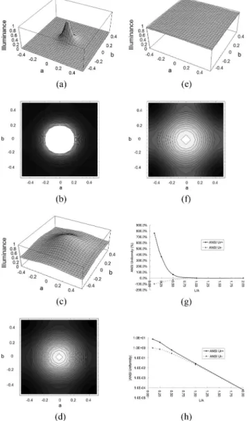
1.00A, and 2.00A, respectively, where A is a constant. The distributions of the illuminances for L⫽ 0.10A, 0.50A, and 1.00A are shown in Figs. 8(a), 8(c), and 8(e), respectively, and the contours of the illumi-nances for L⫽ 0.10A, 0.50A, and 1.00A are shown in Figs. 8(b), 8(d), and 8(f), respectively. The variation of the ANSI light uniformity versus the length L of the light pipe is shown in the linear chart of Fig. 8(g) and in the exponential chart of Fig. 8(h), respectively. The result shows us that the ANSI light uniformity at the exit plane of the light pipe with a single LED light source can be reduced exponentially with the in-crease in the length of the light pipe. In the case of the
length scale L兾A being greater than unity, a single LED source at the center of the entrance plane is uniformly illuminated with the acceptable uniformly brightness image, i.e., ⫹2.7%兾⫺2.16% ANSI light uniformity, on the exit plane of the light pipe. Once the light pipe is long enough with L兾A over 2.0, then the ANSI light uniformity can be achieved to ⫹0.006%兾⫺0.006% as being perfect. This result was also demonstrated and proven in the paper of Cheng and Chern [8] using the semianalytical methods of the sequential ray tracing and the statistical method of the Monte Carlo nonsequential ray tracing. B. Case 2
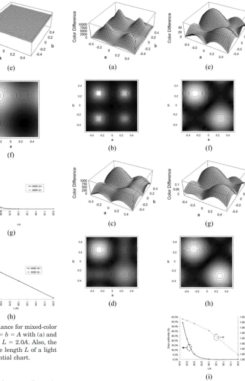
As shown in Fig. 3, the point light sources are located at specific locations on the entrance plane of the light pipe with c ⫽ 0, P ⫽ Q ⫽ A兾4, a ⫽ b ⫽ A,
L ⫽ 0.10A, 0.25A, 0.50A, 1.00A, and 2.00A,
respec-tively, where A is a constant. The distributions of the illuminances for L ⫽ 0.10A, 0.50A, and 2.00A are shown in Figs. 9(a), 9(c), and 9(e), respectively, and the contours of the illuminances for L⫽ 0.10A, 0.50A, and 2.00A are shown in Figs. 9(b), 9(d), and 9(f), respectively. The variation of ANSI light uniformity versus the length L of the light pipe is shown in the linear chart of Fig. 9(g) and in the exponential chart of Fig. 9(h), respectively. The result shows us that the ANSI light uniformity at the exit plane of the light pipe with mixed-color LED light sources can also be reduced exponentially with the increase in length of the light pipe with a similar result as in Case 1. In the case of the length scale L兾A being greater than unity, the mixed-color LED sources on the entrance plane are uniformly illuminated with an acceptable uni-form brightness, i.e., ⫹0.61%兾⫺0.65% ANSI unifor-mity, on the exit plane of the light pipe. Once the light pipe is long enough with L兾A over 2.0, then the ANSI uniformity can be achieved to⫹0.0016%兾⫺0.0016% as being perfect. Furthermore, the distributions of the color differences for L⫽ 0.10A, 0.50A, 1.00A, and 2.00A are shown in Figs. 10(a), 10(c), 10(e), and 10(g), respectively, and the contours of the color differences for L⫽ 0.10A, 0.50A, 1.00A, and 2.00A are shown in Figs. 10(b), 10(d), 10(f), and 10(h), respectively. The variation of the ANSI color uniformity versus the length L of the light pipe is shown in the linear curve and the exponential curve of Fig. 10(i). The result shows us that the ANSI color uniformity at the exit plane of the light pipe with a mixed-color LED light source can also be reduced exponentially by increas-ing the length of the light pipe. In the case of the length scale L兾A being greater than unity, the mixed-color LED sources on the entrance plane are uni-formly illuminated with an acceptable uniform color image, i.e., 0.27% ANSI color uniformity, on the exit plane of the light pipe. Once the light pipe is long enough with L兾A over 2.0, then a perfect ANSI uni-formity can be achieved to 7.3⫻ 10⫺6%.
C. Case 3
As shown in Fig. 3, the point light sources are located at specific locations on the entrance plane of the
Fig. 8. Distributions and contours of illuminance for single LEDs under the condition of P⫽ Q ⫽ 0 and a ⫽ b ⫽ A with (a) and (b)
L⫽ 0.1A, (c) and (d) L ⫽ 0.5A, (e) and (f) L ⫽ 1.0A. Also, the
variation of ANSI light uniformity versus the length L of a light pipe with (g) the linear chart and (h) exponential chart.
light pipe with c ⫽ 0, P ⫽ Q ⫽ A兾4, a ⫽ L ⫽ A,
b ⫽ 0.5A, 1.0A, 1.5A, 2.0A, and 3.0A, respectively,
where A is a constant. The distributions of the illu-minances for b⫽ 1.5A, 2.0A, and 3.0A are shown in Figs. 11(a), 11(c), and 11(e), respectively, and the contours of the illuminance for b ⫽ 1.5A, 2.0A, and 3.0A are shown in Figs. 11(b), 11(d), and 11(f), respec-tively. The variation of the ANSI light uniformity versus the height b of the light pipe is shown in the linear chart of Fig. 11(g) and in the exponential chart of Fig. 11(h), respectively. The result shows us that the ANSI light uniformity at the exit plane of the light pipe with mixed-color LED light sources can also be increased exponentially by increasing the height of the light pipe opposite to that of Case 2. In the case of the height scale L兾A being greater than 2.0, the mixed-color LED sources on the entrance
plane is not able to be uniformly illuminated with an acceptable uniform brightness image, i.e., ⫹6.2%兾⫺5.3% ANSI uniformity, on the exit plane of the light pipe. Furthermore, the distributions of the color differences for b ⫽ 1.5A, 2.0A, and 3.0A are shown in Figs. 12(a), 12(c), and 12(e), respectively, and the contours of the color differences for b ⫽ 1.5A, 2.0A, and 3.0A are shown in Figs. 12(b), 12(d), and 12(f), respectively. The variation of the ANSI
Fig. 9. Distributions and contours of illuminance for mixed-color LEDs in the condition of P⫽ Q ⫽ A兾4 and a ⫽ b ⫽ A with (a) and (b) L⫽ 0.1A, (c) and (d) L ⫽ 0.5A, (e) and (f) L ⫽ 2.0A. Also, the variation of ANSI light uniformity versus the length L of a light pipe with (g) the linear chart and (h) exponential chart.
Fig. 10. Distributions and contours of the color difference for mixed-color LEDs in the condition of P⫽ Q ⫽ A兾4 and a ⫽ b ⫽ A with (a) and (b) L ⫽ 0.1A, (c) and (d) L ⫽ 0.5A, (e) and (f) L ⫽ 1.0A, (g) and (h) L ⫽ 2.0A. Also, (i) the variation of ANSI color uniformity versus the length L of a light pipe with the linear chart and exponential chart.
color uniformity versus the length L of light pipe is shown in the linear curve and the exponential curve of Fig. 12(g). The result shows us that the ANSI color uniformity at the exit plane of the light pipe with a mixed-color LED light source can also be increased exponentially by increasing the height of the light pipe. In the case of the height scale L兾A being greater than 2.0, the mixed-color LED sources on the en-trance plane is not able to be uniformly illuminated with an acceptable uniform color image, i.e., 2.3% ANSI color uniformity, on the exit plane of the light pipe.
D. Case 4
As shown in Fig. 3, the point light sources are located at specific locations on the entrance plane of the light
pipe with c⫽ 0, a ⫽ b ⫽ L ⫽ A, P ⫽ Q ⫽ A兾8, A兾4, 3A兾8, and 1A, respectively, where A is a constant. The distributions of the illuminances for P ⫽ Q ⫽
A兾8, A兾4, 3A兾8, and 1A are shown in Figs. 13(a),
13(c), 13(e), and 13(g), respectively, and the contours of the illuminances for P⫽ Q ⫽ A兾8, A兾4, 3A兾8, and 1A are shown in Figs. 13(b), 13(d), 13(f), and 13(h), respectively. The variation of the ANSI light unifor-mity versus the location of the mixed-color light sources is shown in Fig. 13(i). The result shows us that the ANSI light uniformity on the exit plane of the light pipe with mixed-color LED light sources can also be minimized at⫹0.61%兾⫹0.65% under the con-dition of the locations P⫽ Q ⫽ A兾4. Furthermore, the distributions of the color difference for P ⫽ Q ⫽
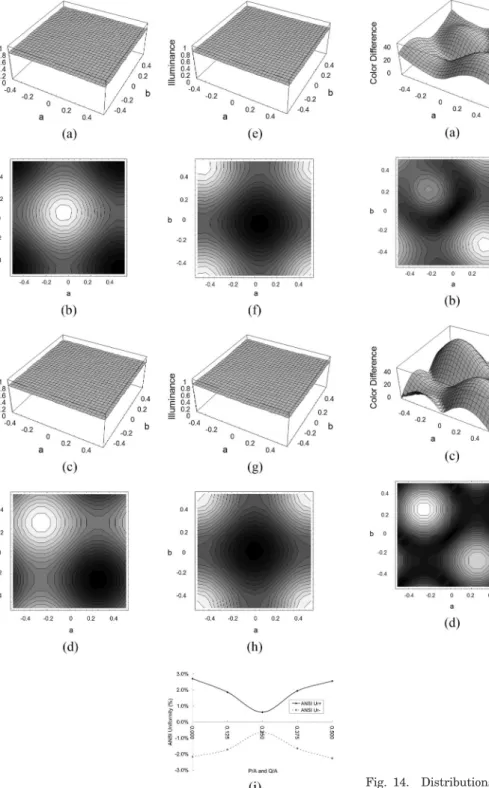
A兾8, A兾4, 3A兾8, and 1A are shown in Figs. 14(a),
14(c), 14(e), and 14(g), respectively, and the contours
Fig. 11. Distributions and contours of illuminance for mixed-color LEDs in the condition of P⫽ Q ⫽ A兾4 and a ⫽ L ⫽ A with (a) and (b) b⫽ 1.5A, (c) and (d) b ⫽ 2.0A, (e) and (f) b ⫽ 3.0A. Also, the variation of ANSI light uniformity versus the height b of a light pipe with (g) the linear chart and (h) exponential chart.
Fig. 12. Distributions and contours of the color difference for mixed-color LEDs in the condition of P ⫽ Q ⫽ A兾4 and a ⫽ L ⫽ A and (a) and (b) b ⫽ 1.5A, (c) and (d) b ⫽ 2.0A, (e) and (f) b ⫽ 3.0A. Also, (g) the variation of ANSI color uniformity versus the height b of a light pipe with the linear chart and exponential chart.
of the color differences for P⫽ Q ⫽ A兾8, A兾4, 3A兾8, and 1A are shown in Figs. 14(b), 14(d), 14(f), and 14(h), respectively. The variation of the ANSI color uniformity versus the locations of the mixed-color light sources is shown in the linear curve and the exponential curve of Fig. 14(i). The result shows us
that the ANSI color uniformity at the exit plane of the light pipe with a mixed-color LED light source can be maximized at 0.27% under the condition of the loca-tions P ⫽ Q ⫽ A兾4 contrary to the case for ANSI uniformity. However, it will be a trade-off between ANSI brightness uniformity and color uniformity for the human eye.
Fig. 13. Distributions and contours of illuminance for mixed-color LEDs in the condition of a⫽ b ⫽ L ⫽ A with (a) and (b) P ⫽ Q ⫽ A兾8, (c) and (d) P ⫽ Q ⫽ A兾4, (e) and (f) P ⫽ Q ⫽ 3A兾8A, (g) and (h) P⫽ Q ⫽ 1A. Also, (i) the variation of ANSI light uniformity versus the locations P and Q of a light pipe with the linear chart and exponential chart.
Fig. 14. Distributions and contours of the color difference for mixed-color LEDs in the condition of a⫽ b ⫽ L ⫽ A with (a) and (b) P⫽ Q ⫽ A兾8, (c) and (d) P ⫽ Q ⫽ A兾4, (e) and (f) P ⫽ Q ⫽ 3A兾8, (g) and (h) P ⫽ Q ⫽ 1A. Also, (i) the variation of ANSI color uniformity versus the locations P and Q of a light pipe with the linear chart and exponential chart.
6. Conclusions
This paper investigated an analytical method of illu-minance formation generated by illumination using a rectangular hollow light pipe and mixed-color LEDs. The corresponding ANSI light uniformity, ANSI color uniformity, and color difference were derived for sin-gle LED and multimixed-color LEDs. The analytical results indicate that the distributions of illuminance and color difference vary with the different geometric structures of the light pipes and the location of the light sources.
In summary, (1) ANSI light uniformity at the exit plane of the light pipe with a single LED light source can be reduced exponentially by increasing the length of the light pipe. (2) Both ANSI light and color uni-formity at the exit plane of the light pipe with mixed-color LED light sources can also be reduced exponentially by increasing the length of the light pipe. In the case of the length scale L兾A being greater than unity, the mixed-color LED sources on the en-trance plane are uniformly illuminated with the ac-ceptable uniform brightness and color images. (3) Both ANSI light and color uniformity at the exit plane of the light pipe with mixed-color LED light sources can also be increased exponentially by in-creasing the height ratio b兾a of the light pipe. (4) The ANSI light uniformity can be minimized while the ANSI color uniformity can be maximized on the exit plane of the light pipe with mixed-color LED light sources under the condition of the multilight-source locations P ⫽ Q ⫽ A兾4 for the cases shown in this paper.
We can conclude that rectangular light pipes pro-vide extremely uniform illuminations with the high-est light efficiency and the most compact package for the optical system with mixed-color LEDs compared to lenses, prisms, and optical diffusers. The optimum form factor of a light pipe is the fact that the cross section is square, that the length scale L兾A is equal to unity, and that the multilight sources are located on positions of A兾4, individually.
This analytical method can be extended for any shape of the light pipe that has a symmetrical cross section, such as a hexagonal cross-sectional shape or an elliptical one, as well as any asymmetrical cross-sectional shape of the light pipe that can generate symmetrical and asymmetrical forms of illuminance and color differences for mixed-color LEDs, respec-tively. For those cases it is difficult to describe the illuminance formation of the specific shaped light pipe using the photometric method, as we did for the rectangular light pipes. However, by utilizing a sim-ulation package, one can easily verify the illumina-tion distribuillumina-tion for any specific light pipe by Monte
Carlo nonsequential ray tracing. An approximating illuminance formation can then be obtained, and one can then calculate and analyze the color uniformity and color difference of the cases.
This work is supported in part by the National Science Council of Taiwan, under project 93-2215-E-009-057. It is also partially supported by the Ministry of Education and Academic Top University program at the National Chiao Tung University, Taiwan.
References
1. D. G. Pelka and K. Patel, “Invited paper: an overview of LED applications for general illumination,” Proc. SPIE 5186, 15–26 (2003).
2. W. Cassarly, “Nonimaging optics: concentration and illumina-tion,” in OSA Handbook of Optics, 2nd ed. (McGraw-Hill, 2001) Vol. III, pp. 2.28 –2.32.
3. C. M. Chang and H. P. D. Shieh, “Design of illumination and projection optics for projectors with single digital micromirror device,” Appl. Opt. 39, 3202–3208 (2000).
4. W. N. Partlo, P. J. Tompkins, P. G. Dewa, and P. F. Michaloski, “Depth of focus and resolution enhancement of i-line and deep-UV lithography using annular illumination,” Proc. SPIE
1927, 137–157 (1993).
5. H. H. Hopkins, “Physics of the fiberoptics endoscope,” in
Endoscopy, G. Berci, ed. (Appleton-Century-Croft, 1976),
pp. 27– 63.
6. T. Hough, J. F. V. Derlofske, and L. Hillman, “Management of light in thick optical waveguides for illumination: an application of radiometric principles,” SAE Tech. Pap. Ser. 940512 (1994). 7. W. J. Smith, Modern Optical Engineering (McGraw-Hill,
2000), pp. 279 –281.
8. Y. K. Cheng and J. L. Chern, “Irradiance formation in hollow straight light pipes with square and circular shapes,” J. Opt. Soc. Am. A 23, 427– 434 (2006).
9. J. F. V. Derlofske and T. A. Hough, “Analytical model of flux propagation in light pipe system,” Opt. Eng. 43, 1503–1510 (2004).
10. F. Zhao, N. Narendram, and J. F. V. Derlofske, “Optical ele-ments for mixing colored LEDs to create white light,” Proc. SPIE 4776, 206 –214 (2002).
11. R. McCluney, Introduction to Radiometry and Photometry (Artech House, 1994).
12. G. Wyszecki and W. S. Stiles, Color Science—Concept and
Methods, Quantitative Data and Formulae (Wiley, 2000),
Chap. 3, pp. 143–167.
13. American National Standard for Audiovisual Systems— Electronic Projection—Fixed Resolution Projectors, ANSI兾 NAPM IT7.228-1997 (American National Standards Institute, 1997).
14. C. M. Cheng and J. L. Chern, “Optical transfer functions for specific-shaped apertures generated by illumination with a rectangular light pipe,” J. Opt. Soc. Am. A 23, 3123–3132 (2006).
15. See http://www.osram-os.com/ostar-projection/technical.php for technical information.
16. Mathematica version 4, Wolfram Research, Inc., 100 Trade Center Drive, Champaign, Ill. 61820-7237, USA.