ELSEVIER
Reliability Engineering and System Safety 57 (1997) 129-142 © 1997 Elsevier Science Limited All rights reserved. Printed in Northern Ireland P l l : S 0 9 5 1 - 8 3 2 0 ( 9 7 ) 0 0 0 3 0 - 6 0951-8320/97/$17.00
The application of Petri nets to failure
analysis
T. S. Liu & S. B. Chiou
Department of Mechanical Engineering, National Chiao Tung University, Hsinchu 30010, Taiwan, ROC (Received 18 March 1996; accepted 23 February 1997)
Unlike the technique of fault tree analysis that has been widely applied to system failure analysis in reliability engineering, this study presents a Petri net approach to failure analysis. It is essentially a graphical method for describing relations between conditions and events. The use of Petri nets in failure analysis enables to replace logic gate functions in fault trees, efficiently obtain minimal cut sets, and absorb models. It is demonstrated that for failure analysis Petri nets are more efficient than fault trees. In addition, this study devises an alternative; namely, a trapezoidal graph method in order to account for failure scenarios. Examples validate this novel method in dealing with failure analysis. © 1997 Elsevier Science Limited.
1 I N T R O D U C T I O N
A variety of methods for failure analysis have been presented, namely, reliability block diagram, failure m o d e and effects analysis, and fault tree analysis. This study presents a failure analysis m e t h o d based on Petri net models. T h e Petri net theory is a graphical m e t h o d using some basic symbols for describing relations between conditions and events. It can represent and analyze the dynamic behaviour of systems. So far, the Petri net model has been used in a variety of applications, e.g., manufacturing systems, computer software and hardware systems.
Petri nets have two types of nodes n a m e d place P and transition T. These nodes are connected by arcs A, i.e., arcs connect transitions to places or places to transitions. Each place may contain one or more tokens. The basic symbols are defined as follows"
©: Place, drawn as a circle. - - - : Transition, drawn as a bar.
: Arc, drawn as an arrow, between places and transitions.
o: T o k e n , drawn as a dot, contained in places.
M o r e o v e r , Peterson [1] defined P, T, and A as:
P = {P~ l P, is a p l a c e , l <- i <- l},
129
where I is a positive integer
T = {T~ I T~ is a transition,1 - i - I} A m ( p x T) U ( T x P).
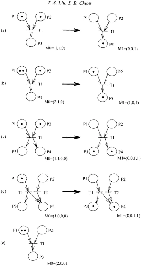
T h e state in Petri nets is represented by a token n u m b e r mi, called a marking, contained in each place Ps. As shown in Fig. l(a), there is a token in each of input places/'1 and P2 but no t o k e n in o u t p u t place P3. Accordingly, the Petri net marking is M = (1,1,0). Each transition connects to both input and output places. A transition is said to be enabled when its every input place contains at least a token. A transition fires if it is enabled, which removes a token from all of its input places and puts a t o k e n in all of its output places. This results in a change of the marking, i.e., a change of the state.
T h e transitions in Fig. l ( a ) - ( c ) are enabled, since in every case both places PI and P2 contain at least one token. A firing of transition T~ moves a token from each of P1 and P2 to the output place P3 (and P4 in case (c)). Place P~ in Fig. l ( b ) originally has two tokens. A f t e r firing, a token remains in PI, since any firing can withdraw only one t o k e n from each input place. In spite of transitions T~ and T2 shown in Fig. l ( d ) , only T~ fires due to its input place Pt, with a token. T h e firing of T~ has nothing to do with input place /)2, whereas it gives a t o k e n to each of P3 and P4- In Fig. l ( e ) , by contrast, T~ is not enabled due to no t o k e n in
t"2.
130 T. S. Liu, S. B. Chiou (a)
Pl~l .~FI P2
MO=( l, 1,0) P1 T1 P2G___)P3
M l
=(0.0.1 ) (b)PI(~~T I P2
MO=(2,
1.0 )
f( P3
P2 Ml=({,O,{) (c)P I ~(~~FI P2
P3
P4
MO=( I, 1,0,0)P1 ~P2
~--
TI
P3
P4
M { =(o,o, {, { ) (d) (e)~)P2
T2
M0=(1.0,0,0)
PI TI~~ ~ P2
T1
T2
P3
P4
M l --(0.0. {, { ) PI T1 P2 MO=(2.0.O)Fig. 1. Firing of transition.
firing (M1) are also illustrated in Fig. 1. The marking in Fig. l(e) is invariant due to no firing, and hence no change of states. When a transition is enabled, it does not necessarily fire immediately but implies a possibility. Petri net modelling methods that involve firing conditions, the time factor, etc. have been developed [2].
The application of Petri nets to reliability engineering has been presented for reliability evaluation [3,4], fault-tolerant analysis [5], safety analysis [6], reliability growth [7], Markov models [8], and stochastic models [9]. The literature used both Petri nets and fault tree analysis methods for software safety analysis [10], fault diagnosis [11], logic
Application of Petri nets
131flowgraph methodology [12], state equation represen- tation of logic operation [13], and analysis of coherent fault trees [14]. The current study presents a matrix method based on Petri nets that are exemplified to outperform fault trees for reliability analysis. In addition, a trapezoidal graph method is devised to facilitate failure analysis and fault detection in the presence of sensors.
2 THE USE OF A PETRI NET TO REPRESENT FAULT TREE
In a manner similar to fault tree analysis, graphical models based on Petri nets can be constructed to
P?
C)
P/
P:
P,
P.~
represent cause-and-effect relationship among events. Since Boolean logic symbols are commonly used to account for failure causation, this work begins with examining logic gates based on Petri nets representation.
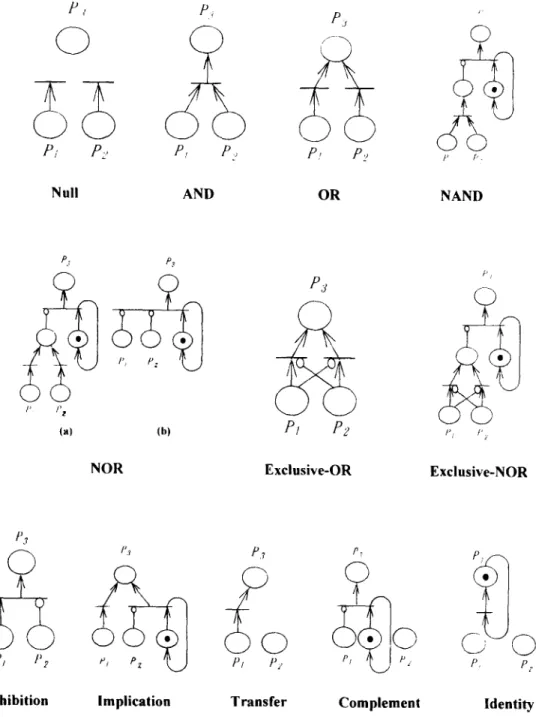
The logic operation for n binary variables requires 2 2" functions. Hence, dealing with two binary variables, the number of Boolean functions is sixteen, among which only twelve functions deserve examina- tion due to repetition of the other four. According to the enabling rules illustrated in Fig. 1, every logic gate can be represented by a Petri net model. The following presents these Petri net models, as shown in Fig. 2, where PI and
P2
are denoted as input places and ~ , the output place of transitions.D j ~
P., P:, ~, r..
Null AND OR NAND
P, P~ I' f'Z (a) (b) P3
Pt
P2
C)
P/ /'ZNOR Exclusive-OR Exclusive-NOR
P3
0
Pl
P2
Inhibition
I'.~ P,~, P 7
Implication Transfer Complement
Fig. 2. Petri net model of logic operation.
P' P2
132 T. S. Lht, S. B. Chiou 1. Null (Ps = 0): P3 never occurs without regard to
the situation of its inputs. There is no arc that connects to any output place, as depicted in Fig. 2.
2. A N D (P3 = P1 P2 = P1 "P2): In Fig. 2, both P~ and Pe must have at least one token [15] to achieve transition firing.
3. O R (P3 = P~ + P2): A t least one of input places must contain at least one token [14] in order to fire, as depicted in Fig. 2.
4. N A N D (P3 = (P~P2)'): As the complement of the A N D function, it needs an inhibitor arc, whose end is always marked by a small circle, at the output place of the A N D Petri net model, combining a self-looped place, as depicted in Fig. 2, to yield inputs of a transition.
5. N O R (P3 = (P~
+ P2)'):
This is the complement of the O R function. As shown in Fig. 2-NOR(a), N O R needs an inhibitor arc at the output place of an O R model, accompanied by a self-looped place to constitute inputs of a transition. This model can be further simplified to become Fig. 2-NOR(b), in which two input places directly connect to the transition by inhibitor arcs.6. Exclusive-OR (P3 = P1P2' + P~P2): A transition fires if either input place contains tokens but does not fire if both input places have one or no tokens. Figure 2 shows that each place inhibits transition firing of the other place, which is linked to an inhibitor arc [1].
7. Exclusive-NOR (P3 = PIP2 + P¢P~): A transition fires if, as illustrated in Fig. 2, both P~ and P2 have tokens or no token.
8. Inhibition (P3 = P~P~): A transition fires if, as illustrated in Fig. 2,/°1 has tokens but P2 has no token.
9. Implication
(P3 -=/°1
+ P~): Fig. 2 depicts that Pj must have tokens or P2 no token to enable a transition to fire.10. Transfer ( P 3 = P 0 : The token in Pt directly transfers to P3 shown in Fig. 2, while without relation with P2.
11. Complement (/°3 = P~): It fires as long as P~ has no token, as depicted in Fig. 2.
12. Identity (P3 = 1): Fig. 2 depicts that place /°3 always contains a token. There is no arc that connects to input places.
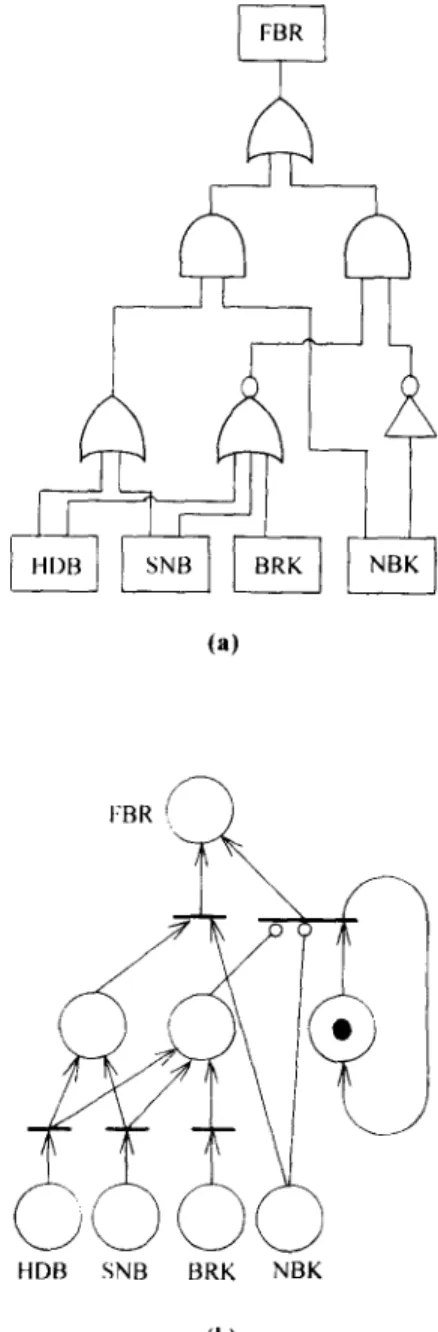
To exemplify the advantage of Petri net models over fault trees, consider a failure event of brake systems used in urban transit vehicles. There are four basic events, namely
1. HDB: holding brake signal 2. SNB: Snow brake signal 3. NBK: No brake demand 4. BRK: Service brake signal.
A logic equation representing the faulty brake event (FBR) of the brake system can be formulated as
FBR = ((HOB + S N B ) . N B K )
+ ((HOB + SNB + B R K ) . N B K ) (1) where denotes NOT. On the right hand side of eqn (1), the term ((HDB + SNB). NBK) account for the situation that the vehicle is not braked although the vehicle is commanded to brake. The other term ((HDB + SNB + B R K . N B K ) ) accounts for the situa- tion that not to brake whereas the vehicle brakes. Either situation represents ,malfunction of the brake system--the top event. Its logic gate model is drawn in Fig. 3(a). Instead, one can resort to its Petri net model as shown in Fig. 3(b) that is constructed based on Fig.
(a)
HDB SNB BRK NBK
(b)
Fig. 3. Model transformation between Logic gate and Petri net.
Application of Petri nets
133 2. Each of four basic places may have a tokendepending on which basic events occur. Enabling rules exemplified in Fig. 1 in turn determine transition firing and token movement. Consequently, if a token is present at the place for
FBR,
system failure is confirmed.Petri nets can also represent condition gates in fault trees, as shown in Fig. 4. An inhibit gate belongs to a synchronized Petri net or interpreted Petri net whose transitions are associated with event E. A delay gate corresponds to a timed Petri net, in which to fire needs a time delay. Moreover, a R out of N gate belongs to a generalized Petri net model with N inputs. The output place will be a median place with weighted input arc R connecting to another transition. When R out of N tokens enter the median place, the transition fires and a token thus enters the output place.
Various event symbols in a fault tree can be replaced by only two simple symbols in a Petri net model, namely, places and steps as shown in Fig. 5. Both basic events and resultant events can be transformed into places. Undeveloped events in fault trees, if necessary, can be replaced by places not to be developed or steps to be developed to other Petri nets. Note that transfer symbols in fault trees are equivalent to steps in Petri net models that serve to simplify Petri net structures.
3 FAILURE PROBABILITY C A L C U L A T I O N
As long as the failure probability of basic events in a fault tree is given, the reliability or failure probability of the top event can he calculated. It is known that calculating failure probability for a fault tree depends on gates. However, for Petri nets it depends on symbols of transitions, places and arcs.
Fault tree
Petri net
Inhibit gate ~ i t i o n ~ E
Fault tree
Petri net
©
event
Undeveloped < ~ ~ )
event (place) (step)
I
Resultant ~ J ~ ' )
event
Transl~r ~ / / ~
Fig. 5. Event symbols and Petri net models.
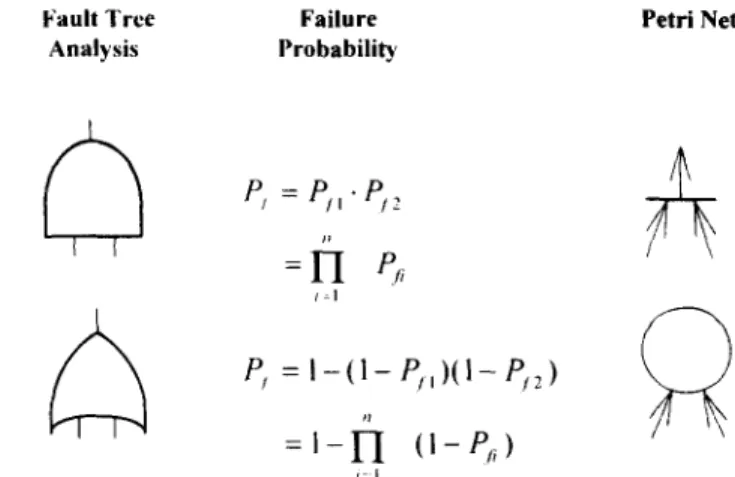
The failure probability Pc in case of a transition with multi-input places can be written as:
Pc = leI Pc,
(2)
i = 1
where
P:i
denotes the failure probability of the ith event. By contrast, the failure probability for a place with multi-input transitions is written as:Pc = 1 - I~I (1 - ~ ) . (3)
i = l
Symbols of gates, Petri nets, and equations for failure probability are shown in Fig. 6. It is not necessary to calculate for the transition or place with single input.
4 MINIMAL CUT SET A N D PATH SET
An approach to generating minimal cut sets for a fault tree was defined by Dimitri [15]. Dealing with the fault tree depicted in Fig. 7, eight steps are required to obtain minimal cut set as listed in Table 1. Using Petri
Fault Tree Failure Petri Net
Analysis Probability
Delay gate ~ e l a y time ~ t
R out of N gate
I
*'* N
Fig. 4. Condition gates and Petri net models.
=FI 6
P, -- t-(l- P,,)(l-
n
= -I1
t=:l
134 T. S. Liu, S. B. Chiou
Fig. 7. Fault tree example.
net models this section provides a new graphic m e t h o d in o r d e r to determine minimal cut sets and path sets. The p r o c e d u r e is described as follows:
1. F o r basic places connected by arcs to reach the top place, if there is no multi-input transition along the arc route, the basic places b e c o m e a minimal cut set.
2. If there exist multi-input transitions along the arc route that connects to the top place, locate their input place by a horizontal arrangement.
3. It is not necessary to deal with any m o r e upper routes in the horizontal arranged place.
4. Replace the horizontal arranged places by their basic places, i.e., the horizontal arranged places will be sub-top places, and repeat p r o c e d u r e 1 to obtain its basic places.
5. R e m o v e supersets whose elements contain elements of other cut sets. This results in the minimal cut set.
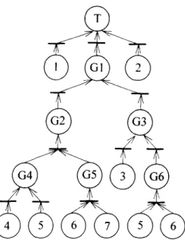
Fig. 8. Petri net corresponding to Fig. 7.
Consider the Petri net depicted in Fig. 8, only three steps, achieved by five c o m p u t e r instructions in total, are required to achieve the minimal cut set as listed in Table 2. T h e underlined numbers in Table 2 show that if u p p e r routes in the horizontal arranged place are considered again (procedure 1(c)), it will still yield the same cut sets as those found in procedure l(b). As a consequence, c o m p a r e d with the fault tree in Fig. 7 that needs eight steps, comprising nine computer instructions, to obtain the minimal cut set, the present Petri net m e t h o d is more efficient.
To find path sets in Petri nets, this study proposes a model n a m e d dual Petri net as shown in Fig. 9. Multi-input transitions of a place can be combined into a transition with multi-inputs connected to the place. Conversely, a multi-input transition can be d e c o m p o s e d into transitions each with an input. After transforming a Petri net into a dual Petri net, minimal path sets can be found by performing the same p r o c e d u r e as that for finding minimal cut sets described above. For example, dealing with the Petri net shown in Fig. 8. its dual Petri net is drawn in Fig.
Table 1. Steps for obtaining cut sets of the fault tree in Fig. 7
Step No. 1 2 3 4 5 6 7 8
No. of instructions for each step Total instruction numbers
GO 1 | 1 1 2 2 2 2 2 G1 G2 G4,G5 G4,G5 G3 G3 3 G6 1 1 1 1 1 9 1 1 1 2 2 4,G5 4,6,7 4,6,7 5,G5 3 3 3 5,6 5,6 5,6 2 1 1
Application o f Petri nets 135
Table 2. Steps for obtaining cut sets of the Petri net in Fig. 8
Step No, 1 2 3
Places
No. of instructions for each step Total instruction numbers l 1 1 2 2 2 4,G5 4,6,7 4,6,7 5,G5 5,6,7 6,7,G4 ~ 7 ~ 6,7,5 3 3 3 5,6 5,6 5,6 2 2 1
10, and three minimal path sets [1,2,3,4,5], [1,2,3,6], and [1,2,3,5,7] are obtained as depicted in Table 3.
J
Fig. 10. Dual Petri net of Fig. 8.
5 A M A T R I X M E T H O D
Minimal cut sets and path sets can he found at the same time using the present matrix method to analyze the Petri net from a top place to basic places. This method proceeds as follows:
1. Write down the numbers of places by making a horizontal arrangement if the output place is connected by multi-arcs to transitions.
2. Write down the numbers of places by making a vertical arrangement if the output place is connected by an arc to a common transition. 3. When all places are replaced by basic places, a
matrix is established. If there is common entry located between rows or columns, it is the entry shared for each row or column, The column vectors of the matrix represent cut sets while row vectors path sets.
4. Remove the supersets to obtain the minimal cut sets and minimal path sets.
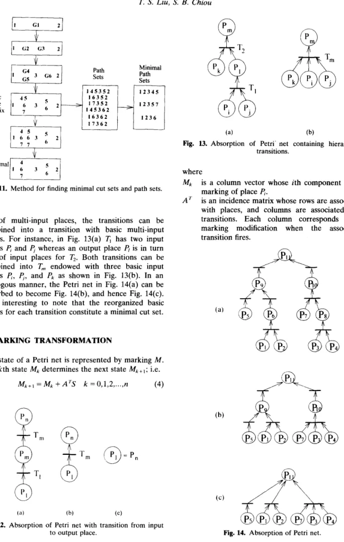
Figure 11 gives an example for the Petri net depicted in Fig. 8. Consequently, minimal cut sets are [1], [2], [3], [5,6], and [4,6,7] while minimal path sets include [1,2,3,6], [1,2,3,4,5], and [1,2,3,5,7]. They are exactly the same as the results in Tables 1 and 3, respectively. The present matrix method is more elIicient than the conventional fault tree in that it is
~ ~ ~ Dual
Fig. 9. Dual Petri net.
not necessary to transform the Petri net into a dual one in order to obtain both minimal cut sets and path sets.
6 A B S O R P T I O N OF P E T R I N E T
A Petri net can be simplified as long as the firing time is not taken into account, i.e., the transfer of a token from an input place to an output place does not take time. When place Pt contains a token as shown in Fig. 12(a), transition T~ satisfies the firing condition. Hence, the token can be moved to place P,,. However, moving a token across transition T~ does not take time, since as depicted in Fig. 12(a) the transition is not timed. Therefore, places Pt and P,,, and transition T~ can be altogether absorbed to become place P~ only, as shown in Fig. 12(b). In a similar manner, a token in place Pt can be subsequently transferred to P, This Petri net model is thus absorbed to become a place P~ = P, as shown in Fig. 12(c).
If a transition has multi-input places, the Petri net can not be absorbed according to the above procedure. In case of hierarchical transitions consist-
Table 3. Steps for obtaining path sets of the Petri net in Fig. 8 Step No. 1 2 3 4,5,G3,1,2 4.5,3,5,1,2 1,2,3,4,5 6,G3,1,2 Places 7,G3,1,2 6,3,6,1,2 1,2,3,6 7,3,5,1,2 1,2,3,5,7
136 T. S. Liu, S. B. Chiou 1 I G2 G3 2 / /
3 "6
2 ] .
Basic I 4 5 5 L Place 6 3 6 2/
Matrix 7+
4 5 5 I Cut I 6 6 3 2 Sets 7 7 6+
Minimal[ "' 4 5 Cut /I 6 3 Sets | 7 6 Path Setsf
_ _ 1 4 5 3 5 2 1 6 3 5 2 1 7 3 5 2 1 4 5 3 6 2 1 6 3 6 2 1 7 3 6 2 Minimal Path SetsFig. 11. M e t h o d for finding minimal cut sets and path sets.
ing of multi-input places, the transitions can be combined into a transition with basic multi-input places. For instance, in Fig. 13(a) T~ has two input places P~ and Pj whereas an output place P~ is in turn one of input places for T2. Both transitions can be combined into T,, endowed with three basic input places P~, ~ , and Pk as shown in Fig. 13(b). In an analogous manner, the Petri net in Fig. 14(a) can be absorbed to become Fig. 14(b), and hence Fig. 14(c). It is interesting to note that the reorganized basic places for each transition constitute a minimal cut set.
7 M A R K I N G T R A N S F O R M A T I O N
The state of a Petri net is represented by marking M. The kth state Mk determines the next state Mk+~; i.e.
Mk+1=Mk+ArS k = 0 , 1 , 2 .... ,n (4)
T m
B y m
(a) (b) (c)
=P°
Fig. 12. A b s o r p t i o n of Petri net with transition f r o m input to o u t p u t place.
(a) (b)
Fig. 13. A b s o r p t i o n of Petri" net containing hierarchical transitions.
where
Mk is a column vector whose ith component is the marking of place P~.
A r is an incidence matrix whose rows are associated with places, and columns are associated with transitions. Each column corresponds to a marking modification when the associated transition fires.
(a)
(b)
Application o f Petri nets 137 S represents a column vector whose ith com-
p o n e n t denotes the firing times of T~.
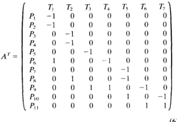
F o r example [14], dealing with the Petri net shown in Fig. 15(a), its incidence matrix becomes:
Combining all marking transformations from an initial marking Mo tO final marking M., eqn (4) can be rewritten as
&In = Mo + A r ~ (5) where
A ' ~ =AM=M,.-Mo
and ~ denotes a firing-count vector.
In Petri nets, w h e n e v e r a t o k e n enters the top place, i.e., when the top event occurs in fault trees, the system becomes faulty. T h e r e f o r e , by letting the last c o m p o n e n t in the marking column vector be the marking of the top place, the final marking Mn for failure analysis is of the form M, = [** . . . . "1] x, where n denotes the nth modification, and * represents the n u m b e r of tokens that are not taken care of in all places other than the top place.
(a)
(b)
Fig. 15. Petri net for illustrating marking transformation and renumbering. A t =
T1
T2
T3
L
r,
T.
Tv
,°1 - 1 0 0 0 0 0 0 P2 - ] 0 0 0 0 0 0 P3 0 - 1 0 0 0 0 0 /'4 0 - 1 0 0 0 0 0 P5 0 0 - 1 0 0 0 0 /°6 1 0 0 --1 0 0 0 Pv 0 0 0 0 - 1 0 0 Ps 0 1 0 0 - 1 0 0 P9 0 0 1 1 0 - 1 0 Pm 0 0 0 0 l 0 - 1 P11 0 0 0 0 0 1 1 (6)Assume an initial marking M0 = [10111010000] v. A firing sequence 7"27"5 T7, i.e., the firing-count vector ~1 = [0100101] 7` transforms Mo to M, = [10001000001] r. In a similar manner, a firing sequence T3T6, i.e. the firing-count vector X2=[0010010] r transforms Mo to M, = [10110010001] r. This study treats the marking as a system state. Thus, the variation of failure states can he delineated by proposed marking transformation.
8 RENUMBERING INCIDENCE MATRIX
This paper proposes an entry arrangement m e t h o d to obtain incidence matrices in a unified manner:
1. Assign numbers to basic places.
2. T h e numbers of places and transitions are the same. If there are multiple input places connected to a c o m m o n transition, the n u m b e r of this transition has as many characters as the n u m b e r of input places.
3. N u m b e r o t h e r output places and transitions. 4. Put the numbers in entries of an incidence
matrix.
5. A p p e n d a column with its last entry as - 1 to the right of the matrix. A square matrix is thus formed.
In fact, the square matrix is a triangular matrix. If there are n basic places and totally l places, the upper-left n × n sub-matrix is a negative identity matrix, while its upper-right n × ( l - n) sub-matrix is a null matrix.
Based on the procedure, the n u m b e r modification of places and transitions is carried out for the Petri net
138 T. S. Liu, S. B. Chiou
model depicted in Fig. 15(a), which results in Fig. 15(b). As a result, its incidence matrix becomes:
A t = T, T2 ~ T, T~ T6 T7 T~ T. T,,, T,11 Pt - 1 0 0 0 0 0 0 0 0 0 0 P2 0 - 1 0 0 0 0 0 0 0 0 0 P3 0 0 - 1 0 0 0 0 0 0 0 0 P4 0 0 0 - 1 0 0 0 0 0 0 0 P5 0 0 0 0 - 1 0 0 0 0 0 0 P~ 0 0 0 0 0 - 1 0 0 0 0 0 P7 0 0 1 1 0 0 - 1 0 0 0 0 Ps 1 1 0 0 0 0 0 - 1 0 0 0 P9 0 0 0 0 1 0 0 1 - 1 0 0 Plo 0 0 0 0 0 1 1 0 0 - 1 0 Pli 0 0 0 0 0 0 0 0 1 1 - 1 (7) This resultant matrix facilitates subsequent marking transformation analysis. It has a simple form and can be used to avoid a wrong firing sequence, since the numbers of places and transitions are the same. Whenever a token appears in P~ it means T~ can fire. In the case of a transition with two input places, there are two characters for numbering. It leads to two entries each with value of 1 in a row. These two entries are underlined for ease of identification. The transition with underlined entries does not fire unless tokens appear in both input places.
Assume an initial marking Mo = [1011010000] 7` and put this vector under the renumbering incidence matrix. As depicted in Fig. 16, the transition ~74 can fire since each of the corresponding places P3 and P4 has a token. The firing of T3 T4 removes the tokens of
A T = PI P6 P7 P8 P9 B0 Ptl - I ' 0 . . . ÷ . . . 0 0 1 1 0 0E-I 0 0 0 0 1 1 0 0 0 0 ! 0 - 1 0 0 0 0 0 0 0 1 0 i 0 1 -1 0 0 0 0 0 0 0 111 0 0 - 1 0 0 0 0 0 0 0 i 0 0 1 1 -1 M 0 = J l O l I 0 1 M , = [ I 0 0 0 0 I M 2 = J I o o o o o [ i o o o o o 0 0 0 0 0 I
lOOOOl
ooo ol
0 0 0 0 1 [Fig.
16. M a r k i n g t r a n s f o r m a t i o n by r e n u m b e r e d i n c i d e n c e matrix.P3 and P4, puts one token in P7 and transforms the marking to become M~ = [100001 10000] z'. In a similar manner, the transition T6T7 can fire since their corresponding places P6 and P7 possess tokens, respectively. The firing of T6T7 removes the tokens of P6 and PT, puts one token in Pro, and transforms the marking to yield/142 = [10000000010] r. Finally, transi- tion T~o fires and ends up with the marking M3 = [10000000001] T. The last entry of this marking turns out to be 1, which represents a system failure.
9 T R A P E Z O I D A L G R A P H M E T H O D
A new diagrammatic method is proposed in this section. Retaining the lower part in the renumbering incidence matrix, as depicted in eqn (7), but excluding the negative identity and null sub-matrices results in a rectangular graph. It contains an ( / - n ) x n sub- matrix and an ( l - n ) × ( l - n) triangular sub-matrix. Deleting further the null part of this triangular sub-matrix yields a trapezoidal graph, shown in Fig. 17.
Every entry with digit of 1 in Fig. 16 can be represented by a thin bar as shown in Fig. 17. However, if in any row with digit of 1 there are entries that have been underlined, the bar is drawn as thick one. Under the trapezoidal graph, write down numbers from 1 to the number of the top place, and write down the numbers of output places beside the numbers of basic places on the left side of this graph. Accordingly, token transformation in the Petri net model can be carried out as follows:
1. Put tokens on the top of the graph if the corresponding numbers of basic places contain tokens.
2. Let the tokens fall down. 3. The tokens will hit the bars.
4. As long as either a thin bar loads a token or a thick bar fully load tokens, a token will roll horizontally to the right hand side.
5. Once the rolling token hits the slope in the graph, it falls down again and may hit a lower bar.
6. Repeat steps 4 and 5 until no token can be rolled any further. • O 0 • 7 ! .... ! m l ... i .... " , , , , i ~ , 9 -~ . . . T - - - ~ - - - ! - --!---~
,o -i ... i
.... : - - ' - - i . . . .!----,,,N
II .-',,, . . . ~, .... ,:-- -:, -'---; "-, ,,B----,' - ' ~ , , I 2 3 4 5 6 7 8 9 10 11 Fig. 1% T o k e n t r a n s f o r m a t i o n using t r a p e z o i d .Application of Petri nets 139
7. If any t o k e n rolls down to reach the n u m b e r of the top place, it represents that the system fails. In the present example, since Mo = [1011010000] 7, each of the basic places /1, P3, P4 and P6 has one token. Thus, put the tokens on the top of the trapezoidal graph. T h e tokens for places P1 and P6 drop, and subsequently stay on their corresponding thick bar. Moreover, the tokens in P3 and P4 also drop and are fully loaded by the thick bar. One of the tokens rolls horizontally to the right hand side, hits the slope and hence drops again. It is in turn loaded by the thick bar that has already loaded a t o k e n coming from P6. T h e bar fully loads tokens now, therefore one of the tokens is allowed to roll to the right until it hits the slope. This t o k e n drops again to hit a lower thin bar. This token rolls out again, hits slope and drops to arrive at n u m b e r 11, i.e., the n u m b e r of the top place. Accordingly, the system fails. F u r t h e r m o r e , it can be seen that simply one event P1 does not cause this system to fail, since it does not constitute a cut set. This fact can also be checked based on the same graph. T o that end, let a t o k e n corresponding to n u m b e r 1 fall down from the graph top. Although the t o k e n is in turn loaded by a thick bar, no subsequent m o v e m e n t can be activated. Suppose, however, event P2, also occurs, P1 and P2 will form a cut set. It is observed that a n o t h e r token falling down from n u m b e r 2 enables a thick bar to fully load tokens. One of the two tokens in turn rolls horizontally to the right. As a consequence, the token drops to reach n u m b e r 11, which accounts for system failure. Hence, the proposed trapezoid m e t h o d has been Verified to be effective.
Note that by either minimal cut sets or logic algorithm methods, the cause and effect relationship among events in a system can not be disclosed. T h e y
can only identify whether events lead to system failure; therefore, they can be treated as 'static' analysis methods. On the contrary, the present novel m e t h o d is capable to account for failure scenarios. T h e t o k e n motion in the trapezoidal graph behaves in a m a n n e r similar to transition firing and token transferring in Petri nets. T h e success of this trapezoidal graph m e t h o d is attributed to its accounting for numbering evolution in the incidence matrix.
10 FAULT DETECTION USING PETRI NETS
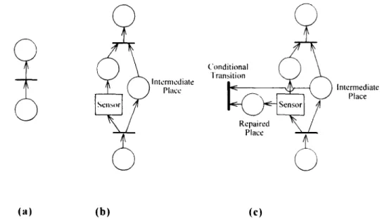
In Petri nets, every place accounts for a state in a system. W h e n a fault tree is transformed into a Petri net model, the presence of tokens in the top place implies that failure occurs. In an a u t o n o m o u s Petri net, a t o k e n may appear in an input place and satisfy the firing condition. As a consequence, the token moves into the output place. A basic failure thus leads to the higher hierarchical failure or serious failure as shown in Fig. 18(a).
In practice, machines and factories may contain sensors to detect failures and prevent basic failure from endangering system safety, for which sensors can be incorporated in Petri nets as shown in Fig. 18(b). W h e n the basic failure occurs, the firing makes a t o k e n enter the intermediate place for isolating, while another t o k e n enters the sensor block to represent detection by a sensor. If the detection is ineffective, the token will leave the sensor block. T h e subsequent firing of a higher hierarchical transition causes the tokens to move into the output place. As a result, failure occurs.
In addition, to model corrective maintenance or replacement of a faulty unit following fault detection, tokens in the intermediate place and the sensor block
)
)
Placed
Intermediate Place (a) (b) (c)140
T. S. Liu, S. B. Chiou
T, ~ T , ;
\,.,o,_.,+.,+~ ~ ° " I , ' ~ '~ ~.,,,o.~
%0 Place
L , ~ , _.~___
I | t I I ~ I 1 ~ I l l(1)
•
•
I I I * I I I I I 9 k ~ + ] • - I - - t ~ - . - L , - I I I I I I I I i ~ . + ~ I t I , . ; - - - . I - ~ * t ,~ [ 0 I - , " T - I - - -- T - q l i l l l i ~ i P " ~ ' - -- ~ - - - ~ I I I I I I I I I 2 3 4 5 6 7 8 9 i0 Iili
+++++
7 8 9 10 11._'-"] x
. . . . ,
_ + , ' r • I - - T I - ' I I r I I 2 3 4 5 6 7 8 9 I0 I1 T g ~ u n d e t e c t c u T [ o _~~
~
T,o
ReP~eed
7 8 9 10 IIt
', i
Ty-
(3)
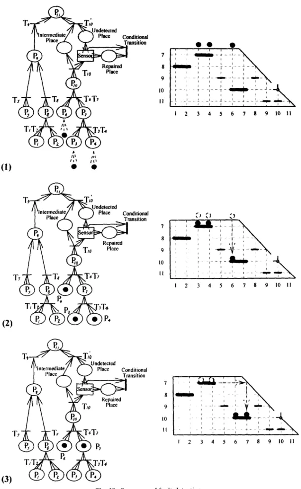
Fig. 19. S e q u e n c e o f fault detection.
_ 1 \
r J J I ! i • , ' ~
Application of Petri nets 141
T g ~
undP~tecaceted
Conditional(4) T~T~ (~T~
7 8 9 10 I1 i ~ i ~ ~ ~ , i"% , , ~ ,"t .d't 4 . ~ l , ] : ~ I I i i i ' '~1 1 2 3 4 5 6 7 8 9 10 II~ U
Tp
"l'tnt~r=~iate/
( ~npd~l~cled
Conditional( 5 ) 10
II
i ; i t - ( - , i i : 1 i [ 1 I 2 3 4 5 6 7 8 9 10 11/l\lnte~r::~d:ateJ / ( ~ Unlqltatce~ted Conditional
I .... ~
"T"
~ Transition
T N T'
( 6 ) ~ . ~ ~ . ~ 7 8 9 10 II , t , ~ t t :_.%
. t . . ! I ¢ m I I I I 2 3 4 5 6 7 8 9 10 11142 T. S. Liu, S. B. Chiou should be eliminated after the failure is repaired. This
can be achieved by installing a conditional transition, as shown in Fig. 18(c), which is connected to both intermediate place and sensor block. If the basic failure has been detected and is under repair, tokens will be put in both intermediate place and repaired place. After the repair work is done, the conditional transition fires, and tokens in both places will move out of the Petri net.
Figures 19 and 20 exemplify fault detection. Suppose that a sensor is employed for detecting a fault that occurs at place Plo and the system has initial marking at P3, P4, and P6 where each contains a token. The firing of transition T3 T4 transfers tokens in both P3 and P4 into a token in place PT. The tokens in P6 and P7 are in turn transferred into a token a t / 1 o due to the firing of T6TT. Consequently, fault arising from P~o can be detected by the sensor, and the token is transferred into an intermediate place. During a maintenance period, a token stays at a repaired place. After repair, tokens located at both intermediate and repaired places vanish due to firing of the conditional transition.
Furthermore, the foregoing scenario of repair activity can also be illustrated using the trapezoidal graph. To that end, as depicted in Fig. 18, make a notch on the slope corresponding to the number of places that represent sensors, and at the notch attach a horizontal inverse L-shaped hinge. When a token rolls to the right hand side on this level, the token will be stopped by the hinge. It dictates that fault is detected by the sensor installed at the corresponding place. Once repaired, the hinge turns clockwise, and the token will roll out of the trapezoid along the slope. This represents the absence of the failure.
I I C O N C L U S I O N
This paper has presented a Petri net method to efficiently obtain minimum cut sets and path sets. Additionally, the proposed matrix method represents a new approach to arranging place numbers so as to obtain both minimum cut sets and path sets.
Place and transition numbers in Petri nets has been modified to result in incidence matrices, which are convenient for marking development, i.e., failure state analysis. Furthermore, by exploiting evolution of renumbering, the renumbered incidence matrix has been transformed into a trapezoidal graph so as to account for system failure scenarios. It is an effective
graphical method capable to undertake the function of Petri nets. Examples have demonstrated that marking transfer, system failure and fault detection can be achieved using this proposed method.
REFERENCES
1. Peterson, J. L., Petri Net Theory and the Modelling of Systems. Prentice-Hall, Englewood Cliffs, New Jersey, 1981.
2. David, R. and Alia, H., Petri net for modelling of dynamic systems-- a survey. Automatica, 1994, 30(2), 175-202.
3. Kumar, V. and Aggarwal, K. K., Petri net modelling and reliability evaluation of distributed processing systems. Reliability Engineering & System Safety, 1993, 41, 167-176.
4. Misra, K. B., New Trends in System Reliability Evaluation. Elsevier Science, Amsterdam, 1993. 5. Viswanadham, N., Reliability of Computer and Control
Systems. Elsevier Science, New York, 1987.
6. Leveson, N. G. and Stolzy, J. L., Safety analysis using petri nets. IEEE Transactions on Software Engineering, 1987, 133, 386-397.
7. Shabalin, A. N., Generation of models for reliability growth. In Proceedings of the 1992 Annual Reliability and Maintenance Symposium, IEEE, New York, pp. 299-302, 1992.
8: Haverkort, B. R. and Trivedi, K. S., Specification techniques for Markov reward models. Discrete Event Dynamic Systems: Theory & Applications, 1993, 3, 219-247.
9. Sahner, R. A. and Trivedi, K. S., A software tool for learning about stochastic model. IEEE Transactions on Education, 1993, 361, 56-61.
10. McGraw, R. J., Shimeall, T. J. and Gill, J. A., Software safety analysis in heterogeneous multiprocessor control systems. In Annual Reliability and Maintenance Symposium 1991 Proceedings, IEEE, New York, pp. 290-294, 1991.
11. Viswanadham, N. and Johnson, T. L., Fault detection and diagnosis of automated manufacturing systems. In Proceedings of the 27th IEEE Conference on Decision and Control, Austin, TX. Vol. 3, pp. 2301-2306, 1988. 12. Muthukumar, C. T., Guarro, S. B. and Apostolakis, G.
E., Logic flowgraph methodology: a tool for modelling embedded systems. In Proceedings of the I E E E / A I A A lOth Digital Avionies Systems Conference, New York, pp. 103-109, 1991.
13. Khan, A. A., State equation representation of logic operations through a petri net. Proceedings of the 1EEE, 1981, 694, 485-487.
14. Hura, G. S. and Atwood, J. W., The use of petri nets to analyze coherent fault trees. IEEE Transactions on Reliability, 1988, 375, 469-474.
15. Dimitri, K., Reliability Engineering Handbook, Vol. 2. Prentice-Hall, Englewood Cliffs, New Jersey, 1991.
![Figure 11 gives an example for the Petri net depicted in Fig. 8. Consequently, minimal cut sets are [1], [2], [3], [5,6], and [4,6,7] while minimal path sets include [1,2,3,6], [1,2,3,4,5], and [1,2,3,5,7]](https://thumb-ap.123doks.com/thumbv2/9libinfo/7504944.116878/7.864.456.805.987.1153/figure-example-petri-depicted-consequently-minimal-minimal-include.webp)