納入環境因素之國家、地區及企業效率與生產力

(1)

納入環境因素之國家、地區及企業效率與生產力

National, Regional and Business

Efficiency and Productivity

with Environmental Factors

研究生：羅時芳 Student：Shih-Fang Lo 指導教授：許和鈞教授 Advisor：Dr. Her-Jiun Sheu

國立交通大學

經營管理研究所

博士論文

A Dissertation

Submitted to Institute of Business and Management College of Management

National Chiao Tung University in Partial Fulfillment of the Requirements

for the Degree of Doctor of Philosophy

in

Business and Management June, 2005

Taipei, Taiwan, Republic of China

(2)

納入環境因素之國家、地區及企業效率與生產力

研究生：羅時芳指導教授：許和鈞教授國立交通大學經營管理研究所博士班中文摘要經濟發展與環境保護必須要相互配合、與時俱進，以達永續發展的目的。本篇論文將以效率與生產力的觀點，探討在加入環境影響因素後，對於國家、地區、與企業整體性的績效評估。對於國家與地區的整體績效評估，本文採實證研究進行；對於企業的整體績效，本文則提供一個概念性的架構，以利實際推廣。在實證研究的部分，本文先以國家為比較基準，使用Malmquist生產力指數，探討東亞十國經濟/環境的整體生產力，為因應京都議定書正式生效對各國可能產生的衝擊，文中環境變數採各國二氧化碳的排放量來進行分析。其後，本文以中國大陸三十一個行政區為例，探討一國中各地區之經濟/環境的整體效率與生產力，環境變數採亞洲褐雲的排放物來進行分析，實證結果發現在考慮環境因素後，經濟迅速發展的東部沿海地區較內陸地區整體績效為高。最後，本文提供一個概念性的架構，以效率的觀點，將環境因素納入企業整體績效評估架構之中，透過這個新架構，企業、投資人、與社會大眾可以容易地瞭解企業的運作，並對企業本身營運的能力、財務健全性與對環境的友善程度做一個整體的評價，各種不同性質的團體亦可經由這個一貫的架構，互相溝通並研擬決策。關鍵詞：效率、生產力、二氧化碳、亞洲褐雲、績效評估架構、績效評估指標

(3)

National, Regional and Business

Efficiency and Productivity

with Environmental Factors

Student：Shih-Fang Lo Advisor：Dr. Her-Jiun Sheu Institute of Business and Management

National Chiao Tung University Abstract

Economics and ecology should be mutually reinforcing to attain sustainable development in modern society. From the perspective of efficiency and productivity, this dissertation studies the performances for multiple organization levels from nation, region, to business taking environmental factors into consideration. Both empirical studies and a conceptual framework for evaluating integrated development for multiple levels of the above entities are presented.

Firstly, this dissertation starts investigating the economic-environmental performance from a nation’s level. Productivity growth of ten Asian countries are analyzed by examining their outputs from economic performance and environmental impact standpoint. Taking CO2

emissions into analysis, productivity growth of these nations are calculated using the Malmquist index.

Secondly, this study focuses on a region’s level. This part analyzes the regional development of China by examining economic performance as well as environmental emissions which cause Asian Brown Clouds. Technical efficiency and productivity changes of thirty-one regions in China are computed. The fast-developing east (coastal) regions

(4)

experience higher technical efficiency and productivity growth than the inland central and west regions economically and environmentally.

Finally, a new conceptual framework for evaluating corporate integrated development through the perspective of efficiency is introduced. Under the proposed framework, businesses, investors, and society can conveniently understand and evaluate corporate holistic performance including its operational competence, financial health, and environmental friendliness. Decisions of different levels and groups can be made with programmed consideration on this proposed analytical ground.

Keywords: Efficiency, Productivity, CO2 Emissions, Asian Brown Clouds, Conceptual

(5)

Acknowledgements

I owe the most overwhelming debt of gratitude to my thesis advisor, Professor Her-Jiun Sheu, for his direction, assistance, and guidance for almost ten years. Words are inadequate to express my thanks to him that I have yet to see the limits of his wisdom, patience, and selfless concern for his students, and especially his pleasant characteristics as a mentor.

I would express special thanks to Professor Jin-Li Hu for providing detailed instructions and suggestions for this dissertation. I would also like to express my gratitude to Professor Hwa-Rong Shen, Professor Chyan Yang, Professor Houn-Gee Chen, Professor Yang Li, Professor Chao-Tung Wen, and Professor Wun-Hwa Chen for their valuable comments which have enriched this dissertation for a great extent. Thanks also due to Ms. Hsiao in the Ph.D. program for her patience handling the process throughout my graduate studies.

Special thanks should be given to others who accompany me but not being mentioned for their friendship and kindness during my years in NCTU. This work is dedicated to my parents for their love and support. My sister Joyce always shares her experience studying abroad during these years, which is great inspiration to my life. Finally, thanks go out to my husband Peter, my best friend, for his companion and encouragement.

(6)

List of Tables

Table 2.1 Summary Statistics of Inputs and Outputs ... 15

Table 2.2 Decomposition of Malmquist Productivity Index without/with CO2 Emissions... 19

Table 2.3 Ranking Change of the Malmquist Index without/with CO2 Emissions ... 20

Table 3.1 Summary Statistics of Inputs and Outputs by Year ... 37

Table 3.2 Summary Statistics of Inputs and Outputs by Area ... 38

Table 3.3 Technical Efficiency Score of Region for Variable Returns to Scale ... 40

Table 3.4 Composition of the Efficiency Frontier for Variable Returns to Scale... 41

Table 3.5 Decomposition of the Malmquist Index without/with Environmental Factors ... 43

Table 4.1 Indicator Examples of Input Data... 59

(8)

List of Figures

Figure 1.1 Research Flow Chart... 4

Figure 2.1 Cumulative Change in the MALM without/with CO2 Emissions for Ten Asian Countries. 17 Figure 2.2 Cumulative Change in the MALM without/with CO2 Emissions for Industrialized APEC Countries ... 17

Figure 2.3 Cumulative Change in the MALM and Its Component for China... 24

Figure 2.4 Cumulative Change in the MALM and Its Component for Japan ... 25

Figure 2.5 Cumulative Change in the MALM and Its Component for NIEs ... 26

Figure 2.6 Cumulative Change in the MALM and Its Component for ASEAN-4... 27

Figure 2.7 Cumulative Change in the MALM and Its Component for Industrialized APEC Countries ... 28

Figure 3.1 Regions of China and Average Per Capita Nominal GDP 1997-2001 (RMB) ... 35

Figure 3.2 The Industry Composition Among Areas (% of GDP in 1997) ... 36

Figure 3.3 Decomposition of Malmquist Index without/with Environmental Factors by Area ... 44

Figure 4.1 Bias in Information Use Caused by Selective Perception... 51

Figure 4.2 The Framework for Evaluation of Corporate Integrated Development ... 55

(9)

Chapter 1 Introduction

1.1 Research Background

Environmental ethics is generally defined as the ethical relationship between human beings and the environment in which we live. There are numerous ethical decisions that human beings make with respect to the environment. For example: From a nation’s level, should our country sign the Kyoto Protocol to make efforts on CO2 reduction? From a

region’s level, should we allow continuing to clear cut the forests for the sake of region’s GDP growth? From a business level, should our company make gasoline powered vehicles to deplete fossil fuel resources, and ignore the new-tech vehicles which can create less emission? Environmental ethics is a new field of moral philosophy, primarily because of the recent emergence of awareness (domestically and internationally) and inter-field research regarding humanity's impacts upon nature and the future.

Economics and ecology should be mutually reinforcing to attain sustainable development in modern society. With the increasing awareness of environmental problems and the demand placed by industrial activities on environmental quality, the control of pollution has become more important for nations, regions, as well as individual companies than ever. Increasingly protective environmental legislation and international agreements with an emphasis on conservation and sustainability of our resources are being introduced in most parts of the world. With this trend of global consciousness and behavior to achieve a cleaner earth, the pressure on each level of organization to improve their ways creating wealth is tightened accordingly. As a result, as a member of global village, we must rethink to change our ways of living completely if the global economy is to become sustainable.

(10)

1.2 Research Objective

The object of this thesis is to study the performances for multiple organization levels from nation, region, to business taking environmental factors into consideration, with efficiency perspective. In the following article, both empirical studies as well as a conceptual framework for evaluating integrated development for a nation, a region and a company are presented. A perspective of efficiency looking at an entity’s work value created in terms of input-output is introduced and applied.

This dissertation starts by the basic concept of estimation methodology used for the following empirical studies in chapter three and four. Data envelopment analysis (DEA) approach and Malmquist productivity index will be introduced to measure technical efficiency and productivity changes for each decision making unit, say for example a country or a region. Alternatives to cope with undesirable outputs are also listed.

The third part of this dissertation investigating the economic-environmental performance from a nation’s level. In the first part of this dissertation, productivity growth of ten Asian countries, namely, China, Japan, the NIEs, and the ASEAN-4, are analyzed by examining their outputs from economic performance and environmental impact standpoint. Productivity growth and its components are calculated using the Malmquist index without/with CO2 emissions. Considering CO2 emissions, a cross-country comparison

analysis is also made accordingly.

The forth part of this dissertation is from a region’s level. Taking China for example, this country has seen the fruit of its rapid economic growth over the past two decades, but severe environmental problems have accompanied this, such as the looming danger of Asian Brown Clouds. This part analyzes the regional development of China by examining economic performance as well as environmental emissions. Technical efficiency and productivity changes of thirty-one regions in China during the period 1997-2001 are

(11)

computed. This part also tests if the fast-developing east (coastal) regions experience higher technical efficiency and productivity growth than the inland central and west regions when both economic growth and environmental factors are concerned.

Ultimately, the economic growth of a nation and its regions are powered from its private sector, say the business operating within. Environmental destructions thus occur with these economic activities to influence our living habitat. In the forth part, a new conceptual framework for evaluating corporate integrated development through the perspective of efficiency is introduced. Under the proposed framework, businesses, investors, and society can conveniently understand and evaluate corporate holistic performance including its operational competence, financial health, and environmental friendliness. Therefore, decisions of different levels and groups can be made with programmed consideration on this pure analytical ground.

1.3 Organization of the Dissertation

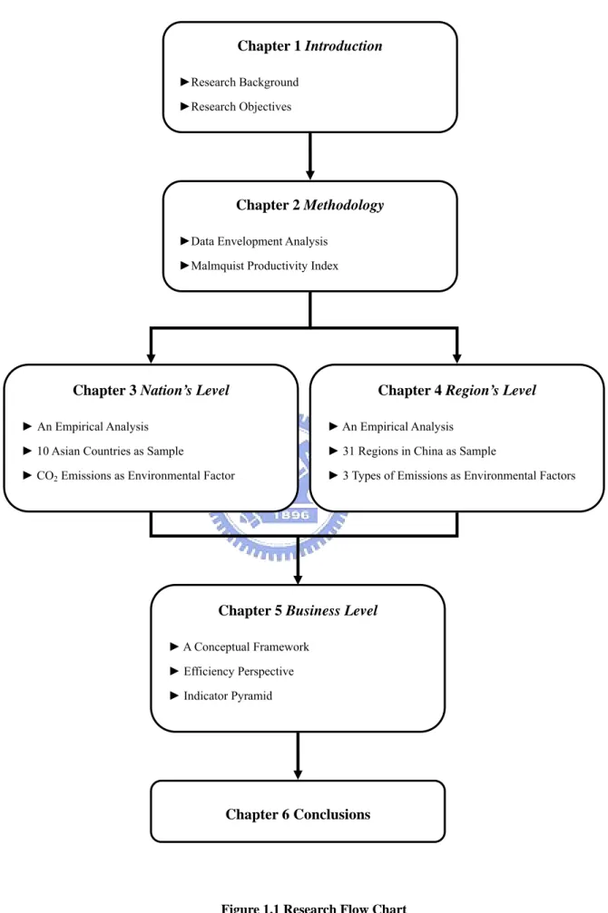
This dissertation is organized in the following manner as Figure 1.1 shows: Chapter 1 presents the motives and objectives of the study. Chapter 2 gives a brief introduction of estimation methodology. Chapter 3 is an empirical analysis taking ten Asian economies as example to investigate the relationship of economic performance and environmental impact. Chapter 4 narrows our scope to the regional performance to a specific country, China. Chapter 5 provides fresh insight on introducing a new framework for the evaluation of corporate integrated development and illustrating its application. Chapter 6 concludes this dissertation.

(12)

Chapter 1 Introduction

►Research Background ►Research Objectives

Figure 1.1 Research Flow Chart Chapter 3 Nation’s Level

► An Empirical Analysis ► 10 Asian Countries as Sample

► CO2 Emissions as Environmental Factor

Chapter 4 Region’s Level

► An Empirical Analysis ► 31 Regions in China as Sample

► 3 Types of Emissions as Environmental Factors

Chapter 5 Business Level

► A Conceptual Framework ► Efficiency Perspective ► Indicator Pyramid

Chapter 2 Methodology

►Data Envelopment Analysis ►Malmquist Productivity Index

(13)

Chapter 2 Methodology

In this chapter the data envelopment analysis (DEA) approach and Malmquist productivity index will be introduced to measure technical efficiency and productivity changes of decision making unit for the following empirical analysis.

2.1 Data Envelopment Analysis (DEA) Approach

DEA is known as a mathematical programming method for assessing the comparative efficiencies of a DMU1 (in this case, a region is counted as a DMU). DEA is a non-parametric method that allows for efficient measurement, without specifying either the production functional form or weights on different inputs and outputs. This methodology defines a non-parametric best practice frontier that can be used as a reference for efficiency measures. Comprehensive reviews of the development of efficiency measurement can be found in Lovell (1993). Assume that there are M inputs and N outputs for each of the K DMUs. For the pth DMU, its multiple inputs and outputs are presented by the column vectors xi and yj, respectively. The technical efficiency score ( ) of DMU p can be found

by solving the following linear programming problem:

p η max (1) η_p s.t.

∑

for i = ≥ − K r r ir ip xλ x 1 0 =1,2, …, M, 0 for j 1 ≥ + −

∑

= K r r jp p jpη y λ y =1,2, …, N, λr ≥0 for r 1,2, …, p, …, K, =

(14)

where η_p is the efficiency score; xi is the ith input; yj is the jth output of the production; and

r

λ is the weight of each observation. The above procedure constructs a piecewise linear approximation to the frontier by minimizing the quantities of the M inputs required to meet the output levels of the DMU p. The weight λr serves to form a convex combination of

observed inputs and outputs. The efficiency score measures the maximal radial expansion of the outputs given the level of inputs. It is an output-orientated measurement of efficiency.

p η

Procedure (1) is also known as the CCR model, named after its authors, Charnes, Cooper, and Rhodes (1978), and it assumes that all production units are operating at their optimal scale of production. Banker, Charnes, and Cooper (1984) suggest an extension of the CRS model to account for variable returns to scale (VRS) situations. This model is called the BCC model, named after its authors. It can be obtained by adding one more constraint on process (1). This constraint essentially ensures that an inefficient DMU is only ‘benchmarked’ against DMUs of similar size. Under the assumption of constant returns to scale (CRS), the results from these two approaches are identical, whereas under variable returns to scale (VRS), the results could be different.

1 1 =

∑

= K r r λ

2.2 Malmquist Productivity Index

Productivity changes can be measured by the Malmquist productivity index, which takes panel data into account. This index was introduced by Caves et al. (1982) who name it the Malmquist productivity index. Sten Malmquist is the first person to construct quantity indices as ratios of distance functions. This method is applied by Färe et al. (1994) to analyze productivity growth of OECD countries, by considering labor and capital as inputs

(15)

and GDP as an output. Chang and Luh (2000) adopt the same method to analyze productivity growth of ten Asian economies. There may be several reasons for the popularity of the Malmquist productivity index. First, the index does not require information on cost or revenue shares to aggregate inputs and outputs, which means it is less data demanding. Second, compared with other productivity indices, the Malmquist index has the advantage of computational ease. And finally, further decomposition of total productivity can be achieved. The Malmquist index could generate output, such as efficiency change and technical change, which could assist in explaining the differences of growth pattern for different countries.

The efficiency measured from the above procedure is static in nature, as the performance of a production unit is evaluated in reference to the best practice in a given year. The shift of the frontier over time cannot be obtained from DEA. To account for dynamic shifts in the frontier, we use the Malmquist productivity index (MALM) developed by Färe et al. (1994). This method is also capable of decomposing the productivity change into efficiency and technical changes, which are components of productivity change.

For each time period t = 1,…, T, the Malmquist index is based on a distance function, which takes the form

Dt _(Xt_{, Y}t₎₌_min﹛_δ_{: (X}t_{, Y}t _/_δ_)∈St_{﹜, (2)}

whereδ determines the maximal feasible proportional expansion of output vector Yt for a given input vector Xt_{under production technology S}t_{at time period t. If and only if the input}

output combination (Xt, Yt) belongs to the technology set St, the distance function has a value less than or equal to one; that is, Dt (Xt, Yt)≤ 1. If Dt _(Xt_{, Y}t₎₌_{1, then the production is on the}

(16)

Caves et al. (1982) originally define the Malmquist index of productivity change between time period s (base year) and time period t (final year), relative to the technology level at time period s:

) ,Y (X D ) ,Y (X D M _s _s _s t t s s ₌ _{. (3)}

It provides a measurement of productivity change by comparing data (combination of input and output) of time period t with data of time period s using technology at time s as a reference. Similarly, the Malmquist index of productivity change relative to technology at time t can be defined as

) ,Y (X D ) ,Y (X D M _t _s _s t t t t ₌ _{. (4)}

Allowing for technical inefficiency, Färe et al. (1994) extend the above models and propose an output-oriented Malmquist index of productivity change from time period s to period t as a geometric mean of the two Malmquist productivity indices of (3) and (4). A CRS technology is assumed to measure the productivity change, and the MALM is expressed as 2 1 CRS CRS CRS CRS MALM _⎥ ⎦ ⎤ ⎢ ⎣ ⎡ = ) ,Y (X D ) ,Y (X D ) ,Y (X D ) ,Y (X D s s t t t t s s s t t s . (5)

Note that if Xs=Xt and Ys=Yt (for example, there has been no change in inputs and outputs between the periods), then the productivity index signals no change when revealing MALM(⋅) 1. Equation (5) of productivity change can be rearranged by decomposing into two components, the efficiency change (EFFCH) and the technical change (TECHCH), which take the following forms:

(17)

) ,Y (X D ) ,Y (X D s s s t t t CRS CRS (EFFCH) change Efficiency = . (6) 2 1 CRS CRS CRS CRS (TECHCH) change Technical _⎥ ⎦ ⎤ ⎢ ⎣ ⎡ = ) ,Y (X D ) ,Y (X D ) ,Y (X D ) ,Y (X D s s t s s s t t t t t s . (7)

The term EFFCH measures the changes in relative position of a production unit to the production frontier between time period s and t under CRS technology. Term TECHCH measures the shift in the frontier observed from the production unit’s input mix over the period.2 How much closer a region gets to the ‘regions’ frontier’ is called ‘catching up’, and is measured by EFFCH. How much the ‘regions’ frontier’ shifts at each region’s observed input mix is called ‘innovation’, shown by TECHCH. Improvements in productivity yield Malmquist indices and any components in the Malmquist index greater than unity. On the other hand, deterioration in performance over time is associated with a Malmquist index and any other components less than unity.

2.3 Coping with Undesirable Outputs

The growth of a nation’s (or a region’s) output depends on capital formation as well as efficiency and productivity improvement. Labor and capital are two major inputs in production. When measuring a nation’s (or a region’s) overall output, gross domestic product (GDP) is commonly used. For a nation/region, while GDP (income) is desirable, emissions (pollutions) are undesirable. The change of income and pollutions are two-way relations: First, the increasing of income deteriorates the environmental condition directly because pollutions are generally byproducts of a production process and are costly to dispose. In reverse, the growth of income is accompanied by public increasing demand for better

(18)

environmental quality through driving forces such as the control measures, technological progress and the structural change of consumption. Desirable GDP and undesirable pollutions should be both taken into account in order to correct a nation’s output. This concept is called ‘green GDP.’ Green GDP is derived from the GDP through a deduction of negative environmental and social impacts.

Data envelopment analysis (DEA) measures the relative efficiency of decision making units (DMUs) with multiple performance factors which are grouped into outputs and inputs. Once the efficient frontier is determined, inefficient DMUs can improve their performance to reach the efficient frontier by either increasing their current output levels or decreasing their current input levels. In conducting efficiency analysis, it is often assumed that all outputs are ‘good.’ However, such an assumption is not always justified, because outputs may be ‘bad.’ For example, if inefficiency exists in production processes where final products are manufactured with a production of wastes and pollutants, the outputs of wastes and pollutants are undesirable (bad) and should be reduced to improve the performance.

There are various alternatives for dealing with undesirable outputs in the DEA framework. The first is simply to ignore the undesirable outputs. The second is either to treat the undesirable outputs in terms of non-linear DEA model or to treat the undesirable ones as outputs and adjust the distance measurement in order to restrict the expansion of the undesirable outputs (Färe et al., 1989). The third is either to treat the undesirable output as inputs or to apply a monotone decreasing transformation (e.g.1 _yb _, _{represents the} undesirable output proposed by Lovell et al., 1995).

b

y

In this study, we treat pollutions as negative externalities which directly reduce output and productivity of capital and labor (López, 1994; Smulders, 1999; de Bruyn, 2000). In other words, the emission proxies used in our analysis are acted as by-product outputs or cost of loss, e.g. the health problem caused, the corrosion of industrial equipment due to polluted air, and other related social expenses. In the following analytical process, we will cope those

(19)

undesirable outputs by two alternatives: taking their reciprocals (applied in chapter 3) as well as taking them as input (applied in chapter 4). In other words, CO2 emissions are taken

their reciprocals to measure a country’s productivity change. Soot, dust, and sulfur dioxide, the main components of Asian Brown Clouds, are considered as input terms to evaluate macroeconomic performance in terms of the regions in China with BCC and Malmquist models.

(20)

Chapter 3 The Asian Growth Experience

3.1 The Economic Growth and CO

2

Emissions in Asia

A country’s macroeconomic policies generally have two objectives: creation of wealth and good living condition for its citizens. Gross domestic product (GDP) is commonly used in assessing a country’s wealth. However, it does not constitute a measure of welfare say for example without dealing with environmental issues adequately. There is necessity to calculate environmental degradation as a correction factor into our regular definition of economic growth (van Dieren, 1995). For the last three decades, Asia has emerged as one of the most important economic regions of the world. Since 1960, the economy of China, Hong Kong, Indonesia, South Korea, Malaysia, Singapore, Taiwan and Thailand together have grown more than twice as fast as the rest of Asia (Angel and Cylke, 2002). As Asia’s economic activities began to shift toward industry and manufacturing, there has been a dramatic increase in pollution in the region (World Bank, 1998). For instance, fast-developing Asia is now one of the major contributors to the global increase in carbon emissions (Hoffert et al., 1998; Siddiqi, 2000). In fact, the highest percentage rises came from the Asia-Pacific region, including India, China and the newly industrializing 'tiger' economies (Masood, 1997). Because emissions of carbon dioxide are generally acknowledged as a cause of ‘global warming,’ the United Nation has been trying to negotiate a global agreement to tackle carbon dioxide emissions. The Kyoto protocol in 1997 was an international milestone of this effort.

The conflict between economic priorities and environmental interests, for a long time, is at the national level since 1960s. However, as Mol (2003) states, there is an increasing clash of economic and environmental institutions, regimes and arrangements at international level

(21)

in recent decades. Studies for economic versus environmental issues is now in a transnational arena. For OECD members, the objective to pursue a balance between pro-development and pro-environment has received considerable attention. Lovell et al. (1995) study the macroeconomic performance of 19 OECD countries by extended data envelopment analysis (DEA) approach, namely Global Efficiency Measure (GEM) for single period analysis. Japan is the only Asian country included in their sample. The study takes four services, real GDP per capita, a low rate of inflation, a low rate of unemployment, and a favorable trade balance as four outputs. When two environmental disamenities (carbon and nitrogen emissions) are included into the service list, the rankings change, while the relative scores of the European countries decline. According to the experience of the OECD countries, environmental indicators do seem to have crucial effects on a nation’s relative performance.

The aim of this chapter is to measure the macroeconomic performance of Asian countries by moderating unwanted externalities of economic growth using panel data over the period 1987-1996. In this study, performance is defined in light of a country’s ability to provide its citizens with both wealth and less polluted environments. We examine the overall performance of ten Asian economies including China, Japan, the East Asian Newly Industrialized Economies (the NIEs, including Hong Kong, Korea, Singapore, and Taiwan), and four countries of the Association of South East Asian Nations (the ASEAN-4, including Indonesia, Malaysia, Philippines and Thailand) by comparing their productivity change. Based on the economic theory of production, productivity is generally defined in terms of the efficiency with which inputs (such as capital and labor) are transformed into outputs (such as gross domestic product, GDP) in the production process. The environmental disamenities are added and the analysis is repeated to see if the performance rankings change. The CO2

(22)

3.2 Data of Asian Countries

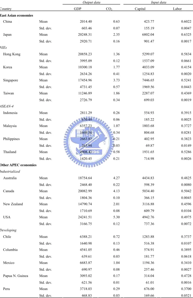
The ten selected Asian countries are all APEC members, thus, we establish a data set of 19 Pacific Rim countries: Australia, Canada, Chile, China, Columbia, Hong Kong, Indonesia, Japan, Korea, Malaysia, Mexico, New Zealand, Papua New Guinea, Peru, the Philippines, Singapore, Taiwan, Thailand, and the United States during the period form 1987 to 1996. We then construct a world frontier based on the data from our country sample. Each country is compared to that frontier. In the analysis without environmental impacts, there are two inputs and one output. We take capital formation and labor force as two inputs and GDP per capita as the only output for a specific country. The data of our multiple comparisons are from Penn World Table Version 6.1 provided by Center for International Comparisons at the University of Pennsylvania (CICUP, 2002). Although capital formation and labor force are not directly available from the data set, simple calculation can be applied. The capital formation is retrieved from the product of real GDP per capita and investment share of real GDP per capita, while the labor force is calculated by dividing real GDP per capita with real GDP per worker. In addition to those two inputs and one output, Table 3.1 transformed CO2

emissions are added into the model. The data of per capita CO2 emissions (metric tons of

carbon) is from Carbon Dioxide Information Analysis Center (Marland et al., 2003). The data after 1996 are not included due to the lack of data for certain countries.

Macroeconomic performance is evaluated in terms of the ability of a country to maximize the desirable output GDP while minimizing the CO2 emissions. The value of

monetary inputs and outputs such as GDP per capita and capital formation are in 1996 international prices. Summary statistics of these inputs and outputs are shown in Table 3.1. The software Deap 2.1 (Coelli, 1996) is applied to solve the linear programming problems.

(23)

Table 3.1 Summary Statistics of Inputs and Outputs

Output data Input data

Country GDP CO2 Capital Labor

East Asian economies

Mean 2014.40 0.63 423.77 0.6022 China Std. dev. 603.46 0.07 155.19 0.0047 Mean 20248.31 2.35 6802.04 0.6325 Japan Std. dev. 2920.71 0.16 901.47 0.0017 NIEs Mean 20858.23 1.36 5299.07 0.5834 Hong Kong Std. dev. 3995.09 0.12 1537.09 0.0661 Mean 10300.18 1.77 4033.09 0.4154 Korea Std. dev. 2634.26 0.41 1254.83 0.0020 Mean 17454.96 3.73 7446.65 0.5241 Singapore Std. dev. 4731.45 0.57 1969.56 0.0443 Mean 11246.89 1.86 2287.07 0.4369 Taiwan Std. dev. 2726.79 0.34 699.03 0.0019 ASEAN-4 Mean 2811.29 0.26 554.93 0.3915 Indonesia Std. dev. 670.49 0.06 185.22 0.0025 Mean 6357.23 1.07 1803.68 0.3727 Malaysia Std. dev. 1669.54 0.34 804.68 0.0281 Mean 2663.87 0.21 402.95 0.3823 Philippines Std. dev. 263.94 0.03 69.87 0.0149 Mean 4908.42 0.58 1931.65 0.5286 Thailand Std. dev. 1420.45 0.21 714.98 0.0026

Other APEC economies

Industrialized Mean 18754.64 4.27 4434.83 0.4825 Australia Std. dev. 2468.40 0.22 598.39 0.0080 Mean 20082.99 4.13 5034.40 0.5042 Canada Std. dev. 1804.36 0.10 366.15 0.0045 Mean 14790.74 2.01 3116.88 0.4596 New Zealand Std. dev. 1710.69 0.08 609.79 0.0104 Mean 24241.51 5.30 4942.76 0.4975 USA Std. dev. 3166.75 0.12 737.36 0.0072 Developing Mean 6388.21 0.72 1283.88 0.3737 Chile Std. dev. 1640.98 0.13 516.38 0.0107 Mean 4541.05 0.46 574.91 0.3895 Columbia Std. dev. 639.61 0.03 181.77 0.0618 Mean 6683.87 1.04 1194.36 0.3410 Mexico Std. dev. 690.97 0.08 257.46 0.0027 Mean 3093.02 0.17 314.04 0.4728 Papua N. Guinea Std. dev. 621.56 0.01 61.01 0.0016 Mean 3718.03 0.29 676.00 0.3700 Peru Std. dev. 468.83 0.03 169.66 0.0521

(24)

3.3 Results of Productivity Change

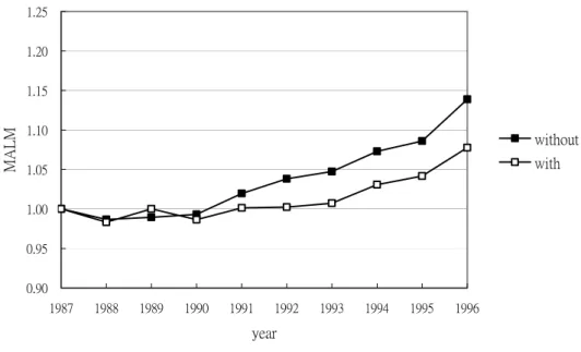
Using the method in section 2.1, the average cumulative changes of ten Asian economies’ productivity without/with CO2 emissions are shown in Figure 3.1, with the year

1987 as the reference year. The overall productivity growth without/with emissions are rising. The trends go up steadily from 1990 to the end of the sample period. The productivity growth with CO2 emissions is below that without CO2 emissions every year

except in 1989. It is to be noted that the gap between these two trends seems to be widening each year. In 1996, the difference almost mounts to six percent. This phenomenon is a contrast with the productivity patterns of the industrialized APEC countries in our sample. Figure 3.2 shows the average cumulative productivity without/with CO2 emissions changes of

Australia, Canada, New Zealand and the USA. The two lines of industrialized APEC countries are almost identical, indicating a relatively stable performance without/with including environmental factors comparing with the East Asian experience. Therefore, the productivity of fast developing Asian economies is not as high as reported after considering other non-economic variables. This result is consistent with the estimation that the rapid growth of Asian economies might take a toll on the environment.

(25)

0.90 0.95 1.00 1.05 1.10 1.15 1.20 1.25 1987 1988 1989 1990 1991 1992 1993 1994 1995 1996 year MA LM without with

Figure 3.1 Cumulative Change in the MALM without/with CO2 Emissions for Ten Asian Countries

0.90 0.95 1.00 1.05 1.10 1.15 1.20 1.25 1987 1988 1989 1990 1991 1992 1993 1994 1995 1996 year MA L M _without with Figure 3.2 Cumulative Change in the MALM without/with CO2 Emissions for Industrialized APEC

(26)

Further comparisons taking into account CO2 emissions among countries are displayed

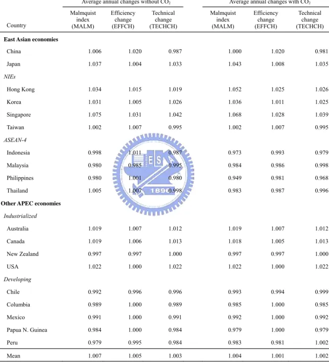
in Tables 3.2. On the left half side of Table 3.2, the average Malmquist index without CO2

emissions of the total sample is 1.007, with 7 Asian countries’ indices exceeding unity implying that they have positive production growth. Singapore has the highest productivity growth, followed by China, Japan and the NIEs. The productivity growth of ASEAN-4, except Thailand, shows deterioration. We then repeat the computation again by adding transformed CO2 emissions as environmental proxies. On the right half side of Table 3.2 is

the average Malmquist index with CO2 emissions with total sample mean of 1.004. Not only

the average Malmquist index is lower than that without CO2 emissions, so are efficiency

change and technical change indices. Among the East Asian economies, while the Malmquist indices of China, Japan and the NIEs still perform positive, that of all ASEAN-4 countries declines. Singapore is the best performer without or with the environmental factors. Between our experiments without/with CO2 emissions, it is clear from Table 3.3 that

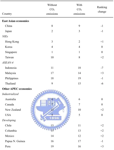
the ranking based on the 10-year average growth performance remain average unchanged, except Indonesia and Thailand, whose ranking regress rather significant compared with other countries’ after taking environmental factors into account. Among the ten Asian economies, those countries with per capita GDP exceeding 10,000 US dollars, such as Singapore, Japan and Hong Kong, generally rank higher no matter whether environmental factor is considered or not.

Lovell et al. (1995) shows that the inclusion of two environmental indicators drastically changes the ranking, reflecting that the environment is a decisive variable when assessing a country’s relative performance for OECD countries. Whether environmental factors are unimportant to a comparison of Asian economies because of average unchanged productivity ranking deserves further study. The ‘Environmental Kuznets Curve’ provides a way to explain this phenomenon. The countries with lower per capita GDP are on the increasing stage of per output pollution. On the contrary, countries with higher per capita GDP report a

(27)

decrease in the per output pollution. It could therefore be stated that better environmental performance has been accompanied with economic achievement for richer countries.

Table 3.2 Decomposition of Malmquist Productivity Index without/with CO2 Emissions

Average annual changes without CO2 Average annual changes with CO2

Country Malmquist index (MALM) Efficiency change (EFFCH) Technical change (TECHCH) Malmquist index (MALM) Efficiency change (EFFCH) Technical change (TECHCH)

China 1.006 1.020 0.987 1.000 1.020 0.981 Japan 1.037 1.004 1.033 1.043 1.008 1.035 NIEs Hong Kong 1.034 1.015 1.019 1.052 1.025 1.026 Korea 1.031 1.005 1.026 1.036 1.011 1.025 Singapore 1.075 1.031 1.042 1.068 1.028 1.039 Taiwan 1.002 1.007 0.995 1.002 1.007 0.995 ASEAN-4 Indonesia 0.998 1.011 0.987 0.973 0.993 0.979 Malaysia 0.980 0.985 0.995 0.984 0.986 0.998 Philippines 0.980 1.001 0.980 0.949 0.981 0.968 Thailand 1.005 1.007 0.998 0.983 0.987 0.996

Industrialized Australia 1.019 1.007 1.012 1.019 1.007 1.012 Canada 1.019 1.006 1.013 1.018 1.005 1.013 New Zealand 0.997 0.997 1.000 0.997 0.997 1.000 USA 1.022 1.000 1.022 1.022 1.000 1.022 Developing Chile 0.992 0.996 0.996 0.993 0.994 0.999 Columbia 0.989 1.000 0.989 0.985 1.000 0.985 Mexico 0.991 1.000 0.991 0.992 1.000 0.992 Papua N. Guinea 0.984 1.000 0.984 0.979 1.000 0.979 Peru 0.979 0.995 0.984 0.983 0.981 1.002 Mean 1.007 1.005 1.003 1.004 1.001 1.002

(28)

Table 3.3 Ranking Change of the Malmquist Index without/with CO2 Emissions Country Without CO2 emissions With CO2 emissions Ranking change

China 8 9 -1 Japan 2 3 -1 NIEs Hong Kong 3 2 +1 Korea 4 4 0 Singapore 1 1 0 Taiwan 10 8 +2 ASEAN-4 Indonesia 11 18 -7 Malaysia 17 14 +3 Philippines 18 19 -1 Thailand 9 15 -6

Industrialized Australia 6 6 0 Canada 7 7 0 New Zealand 12 10 +2 USA 5 5 0 Developing Chile 13 11 +2 Columbia 15 13 +2 Mexico 14 12 +2 Papua N. Guinea 16 17 -1 Peru 19 16 +3

3.4 Results of Cross-Country Comparison

What causes some countries to perform better economically and environmentally than the other countries is an issue to be studied. Without/with considering CO2 emissions, a

cross-country comparison is made for further exploration. The ten Asian economies are studied into groups. The NIEs and the ASEAN-4 are grouped for the countries’ geographical and economical proximity. China and Japan are singled out individually. In other words, the following analysis is made based on China, Japan, the NIEs and the ASEAN-4

(29)

respectively. The industrialized APEC countries, including Australia, Canada, New Zealand and the USA, are incorporated as a comparison basis to Asian economies.

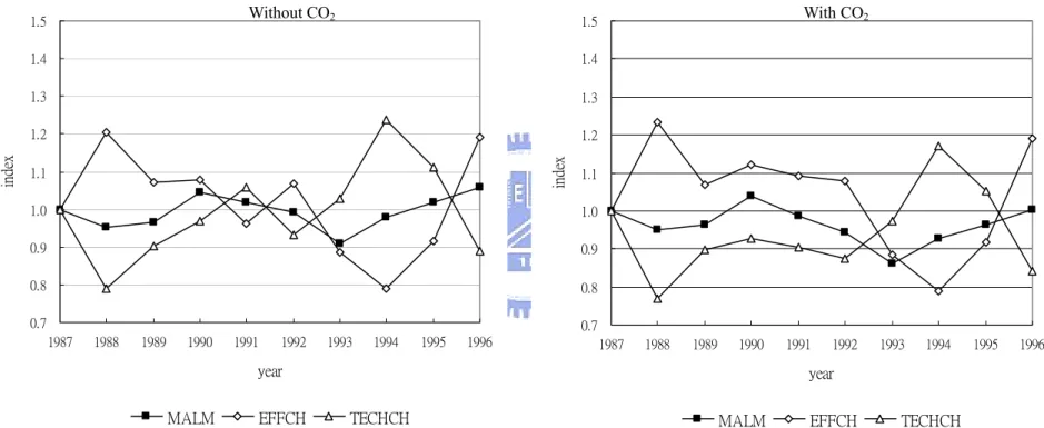
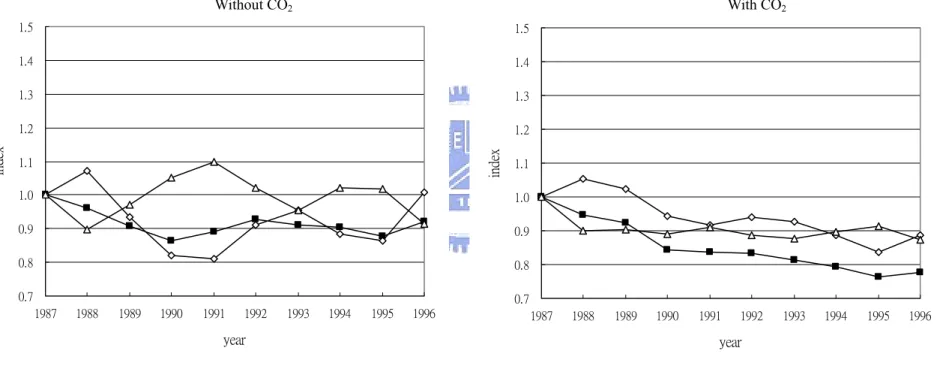
Figure 3.3 shows the cumulative changes in productivity and its components for China. Without/with CO2 emissions, the productivity growths (MALM) show similar patterns:

increases from 1987 to 1990, decline from 1990 to 1993, and increase again after 1993. However, the changes of the MALM with CO2 emissions are more undesirable, i.e., the

increase is slower and decrease faster than which only considered the GDP after 1990. Considering CO2 emissions, it was observed that the two components of MALM, EFFCH and

TECHCH, fluctuate erratically. While the EFFCH rises from 1987 to 1988, it decreases from 1988 to 1994 then reverses from 1994 to 1996, the TECHCH moves almost to the same extent but in a reverse direction. The TECHCH with CO2 emissions is always less than that

without CO2 emissions, indicating that technical change may be overestimated when

considering only economic aspects. The EFFCH shows little different between the two plots. No matter whether the environment is taken account or not, the result suggests that China experiences either technical regress or efficiency loss, and hence deterioration in productivity during our sample period. In other words, lacking of catching-up and innovation capacities in turns encumbers the productivity growth for China. Furthermore, there exists an overestimation for China’s technical change when environmental factors are considered.

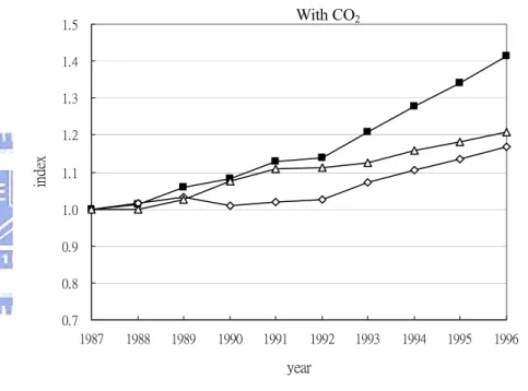
As for Japan (see Figure 3.4) the MALM index increases rapidly from 1987 to 1991 and extends steadily from 1991 to 1996 without/with CO2 emissions. Before 1991, both EFFCH

and TECHCH contribute to the growth of productivity. After 1991, the advance in technical change dominates the stability of efficient change leading to positive growth in productivity. It is worth noticing that the cumulative MALM with CO2 emissions is even higher than that

without CO2 emissions in every year. The difference after considering emissions comes

(30)

input resources compared with other economies. In other words, Japan performs rather well in catching-up to the frontier due to fewer emissions.

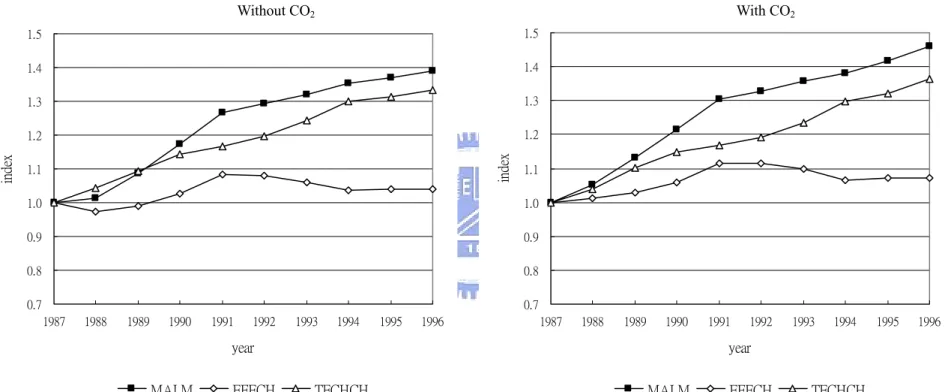
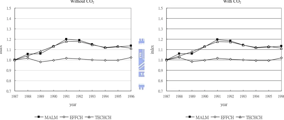
The MALM index of the NIEs (see Figure 3.5) increases by about 40 percent over the years from 1987 to 1996 without/with CO2 emissions, indicating a rapid productivity growth,

especially after 1992. Before 1992, the MALM is dominated by the TECHCH, indicating that the productivity growth is mainly due to improvements in technology. After 1992, the rapid growth of MALM is due to the steady increase of TECHCH and the speedy increase of EFFCH. This implies that the average efficiency of the NIEs countries catches up with the world frontier after 1992. Like Japan, the cumulative MALM with CO2 emissions is even

higher than that without CO2 emissions in every year after 1990. The difference after

considering emissions also comes from the higher cumulative EFFCH growth. In general, after considering environmental factors, the general productivity growth of the NIEs performs even better due to the efficiency progress.

The cumulative changes in productivity and its components for ASEAN-4 are shown in Figure 3.6. Without CO2 emissions, the productivity of ASEAN-4 countries decreases from

1987 to 1990, and remains rather inactive afterwards. The productivity trend with CO2

emissions shows a similar tendency but in a less active manner, implying an overestimation of the ASEAN-4’s productivity when neglecting the environmental impact. The TECHCH fluctuates less with CO2 emissions than without, and so does the EFFCH. When taking

environment variable into account, the MALM is affected by the deterioration of both EFFCH and TECHCH throughout the sample period, indicating the lack of catching-up as well as innovation affects the growth of productivity.

Incorporating the industrialized APEC countries (see Figure 3.7), without/with taking account CO2 emissions, the patterns of MALM and its components show almost no difference.

It could be concluded that the industrialized APEC countries are relatively more economic-environmental balanced than Asian economies. In summary, Japan and the NIEs

(31)

perform even better after considering CO2 emissions because of their higher productivity

growth during the time of our sample period. Emissions can be dealt as undesirable outputs that imply inefficiency. From the experience of Japan and the NIEs, the better productivity growth is because of greater EFFCH defined as their ability to well allocate resources with fewer emissions. On the other hand, the productivity of China and the ASEAN-4 are overestimated when only focusing on GDP from our results. Taking environment into consideration, the productivity growth gets worse because of the fluctuating EFFCH or TECHCH in turns in China. As for the ASEAN-4, the productivity deteriorates due to inactive EFFCH and TECHCH. The Environmental Kuznets Curve hypothesis is mirrored in our cross-country comparison for the productivities of those economies with higher GDP per capita. They perform better both economically and environmentally. Furthermore, the conclusions of this section can serve as encouragement to forge a greater link between the economy and environment.

(32)

0.7 0.8 0.9 1.0 1.1 1.2 1.3 1.4 1.5 1987 1988 1989 1990 1991 1992 1993 1994 1995 1996 year inde x

MALM EFFCH TECHCH

0.7 0.8 0.9 1.0 1.1 1.2 1.3 1.4 1.5 1987 1988 1989 1990 1991 1992 1993 1994 1995 1996 year inde x

MALM EFFCH TECHCH

With CO2

Without CO2

(33)

0.7 0.8 0.9 1.0 1.1 1.2 1.3 1.4 1.5 1987 1988 1989 1990 1991 1992 1993 1994 1995 1996 year in de x

MALM EFFCH TECHCH

0.7 0.8 0.9 1.0 1.1 1.2 1.3 1.4 1.5 1987 1988 1989 1990 1991 1992 1993 1994 1995 1996 year inde x

MALM EFFCH TECHCH

With CO2

Without CO2

(34)

0.7 0.8 0.9 1.0 1.1 1.2 1.3 1.4 1.5 1987 1988 1989 1990 1991 1992 1993 1994 1995 1996 year inde x

MALM EFFCH TECHCH

0.7 0.8 0.9 1.0 1.1 1.2 1.3 1.4 1.5 1987 1988 1989 1990 1991 1992 1993 1994 1995 1996 year inde x

MALM EFFCH TECHCH

Without CO2 With CO2

(35)

0.7 0.8 0.9 1.0 1.1 1.2 1.3 1.4 1.5 1987 1988 1989 1990 1991 1992 1993 1994 1995 1996 year inde x

MALM EFFCH TECHCH

0.7 0.8 0.9 1.0 1.1 1.2 1.3 1.4 1.5 1987 1988 1989 1990 1991 1992 1993 1994 1995 1996 year in de x

MALM EFFCH TECHCH

(36)

0.7 0.8 0.9 1.0 1.1 1.2 1.3 1.4 1.5 1987 1988 1989 1990 1991 1992 1993 1994 1995 1996 year in de x

MALM EFFCH TECHCH

0.7 0.8 0.9 1.0 1.1 1.2 1.3 1.4 1.5 1987 1988 1989 1990 1991 1992 1993 1994 1995 1996 year in de x

MALM EFFCH TECHCH

(37)

3.5 Sub-Conclusions

A country’s development performance could be biased when neglecting a number of important respects such as environmental factors. Since late last century, Asia has emerged as one of the most important economic regions of the world. However, there is wide debate over Asia’s rapid development and sacrifice of its environment. Incorporating environmental consideration into economic orientation opens up a new way of pursuing sustainable development for Asian economies. In this study, performance is defined in terms of a country’s ability to maximize its citizen’s wealth as well as to protect the environment through fewer emissions. The macroeconomic performances of ten Asian economies over the period 1987-1996 are studied. Nineteen APEC member economies are included so as to construct a benchmark frontier. The relative productivity change and its decomposition, including efficiency change (which is defined as catching-up) and technical change (which is defined as innovation), of these ten Asian countries are studied. The analysis is repeated again by incorporating CO2 emissions.

The empirical results could be summarized as follows: (i) Overall, the productivity growth without/with incorporating CO2 emissions shows similar tendency for ten Asian

economies. However, the productivity growth trend with CO2 emissions is below that

without CO2 emissions. The gap between these two trends widens from 1990 to the end of

the sample period. Taking the other industrialized APEC economies as a contrast, a relatively unchanged growth trend is shown after including environmental factors. (ii) Between our analyses without/with CO2 emissions, the ranking of growth performance remain

generally unchanged except in Indonesia and Thailand, who regress rather significant after taking into account environmental factors. (iii) Those Asian countries with higher per capita GDP also tend to rank higher no matter whether the environment is considered or not. (iv) A

(38)

cross-country comparison is made by scrutinizing the growth pattern varies among countries. Taking CO2 emissions into account, Japan and the NIEs experience even better growth

productivity due to higher efficiency progress. (v) For China, either technical regress or efficiency loss leads to deterioration in productivity. For the ASEAN-4, the productivity decline/stagnation is due to the inactive efficient and technical change. The Environmental Kuznets Curve hypothesis can be verified by lesser emissions having been induced with economic achievement for richer countries. The notion that Asia’s rapid growth has been at the expense of its environment needs to be re-analyzed, because from our research this only stands for those economies with lower GDP per capita. In order to promote economic growth and environmental friendliness for Asian countries, especially China and ASEAN-4, the priority should lie in their catching-up capabilities, such as better resource-allocation, and greater innovation related to advanced technologies on the road to sustainable development.

In the long term, growth without environmental protection could lead a country’s industry to be less competitive under the rising pressure from environmental protection requirement from the world trading partners. From our results of Asian growth experience, the overall performances of Japan and the NIEs tend to rank higher both economically and environmentally. This implies that these countries have the potential to have a higher standard both on productivity and environmental quality. During our sample period, China and the ASEAN-4 comparably lagged behind on both efficiency and technical change aspects, implicating that the objective of maximizing wealth while protecting environment needs more efforts and research.

(39)

Chapter 4 The Unbalanced Regional Productivities in China

4.1 Asian Brown Clouds

A three-kilometer thick cloud of toxic pollution looming over Asia, known as ‘Asian Brown Clouds’, caught global concern at the 2002 World Summit on Sustainable Development in South Africa. This thick layer of haze that hangs over a wide expanse of territory covering south to east Asia (South Asia, India, Pakistan, Southeast Asia, and China) is a direct result of damaging development trends (CNN News, 2002), for which the whole world now has to work together so as to help reverse it. Asian Brown Clouds are made of soot, ash, dust, and airborne chemicals, which are all products of man-made pollutions. This toxic haze could kill hundreds of thousands of people prematurely and cause deadly flooding and drought. Scientists warn the impact could be global since winds can push pollutants halfway around the world, including to Europe and even the Americas in a week, according to Concept Paper on Asian Brown Clouds (2001). Therefore, Asian Brown Clouds are not only an important subject for China and its people, but also for all the people of the world.

Ever since China adopted the policy of economic reform and opened up to the outside world in the late 1970s, it has experienced double-digit growth. Although China has experienced rapid economic growth for more than a decade, its environment is rapidly deteriorating. Soot, dust, and sulfur dioxide, the main components of Asian Brown Clouds, are the major pollutants being emitted. Only recently has the Chinese government taken action to cope with these environmental problems, especially on air and water pollution (World Bank, 2001). Although the dust emission has declined, sulfur dioxide and soot emissions have been climbing in recent years (Liu, 2001), and these problems can be

(40)

attributed to old-fashioned and inefficient technology, as well as highly polluting engines and fuels (Ramanathan and Crutzen, 2001).

There are numerous theoretical and empirical studies considering the relationship between economic development and environmental quality --- the famous Environmental Kuznets Curve (EKC) postulates an inverted-U relationship between economic growth and pollution. It suggests that environmental degradation should increase at low incomes, reach a peak (turning point), and eventually decrease at high income. EKC implies that persistent economic growth can be accompanied by reductions of environmental degradation in the long run (Neumayer, 1999). The other optimistic view, the Porter hypothesis, states that reducing environmental impacts of production will improve productivity, hence simultaneously benefiting economic growth and the environment (Porter and van der Linde, 1995). Furthermore, more profitable firms are more likely to adopt clear technologies (Dasgupta et al., 2002). This arouses our curiosity: Do China’s fast-developing east regions both economically and environmentally perform better than the less-developing inland ones? Do their rankings in regional productivities drastically change after taking into account environmental factors? After its entrance into the World Trade Organization (WTO) in 2001, problems of rising regional economic disparities and environmental protection have become more imminent to China.

Incorporating the economy and the environment together, the concept of sustainable development has become a key element of policies not only at national levels, but also at regional levels (Gibbs, 1998). One can recall the old radical green slogan “think globally, act locally.” In other words, development towards sustainability can be introduced by starting from areas on a local or regional level (Wallner et al., 1996; Dryzek, 1997). This type of sub-national scale can be emphasized as a key site for the integration of economic and environment policy (Gibbs, 2000). This would seem to be of particular importance to various regions in China, in light of their geographical and economic diversity.

(41)

4.2 Regional Economic Disparities in China

From the perspective of China’s development and political factors, its provinces, autonomous regions, and municipalities are usually divided into three major areas: the east, central, and west. The east area stretches from the province of Liaoning to Guangxi, including Shandong, Hebei, Jiangsu, Zhejiang, Fujian, Guandong, and Hainan, and the municipalities of Beijing, Tianjin, and Shanghai. Among the three major areas, the east area has experienced the most rapid economic growth. In the early 1980s, the Chinese government established and opened up four special economic zones and fourteen coastal cities to foreign investment and trade. Since then, the special economic zones and the coastal open areas have enjoyed considerable autonomy, special tax treatment, and preferential resource allocations (Litwack and Qian, 1998). They have attracted the most foreign capital, technology, as well as managerial know-how. Rapid economic growth has made this area a magnet for attracting investment and migrant workers. The central area consists of Heilongjiang, Jilin, Inner Mongolia, Henan, Shanxi, Anhui, Hubei, Hunan, and Jiangxi. This area has a large population and a home base of farming. Foreign investment in this area is not as much as in the east coastal regions, and existing equipment relatively lags behind. The west area covers more than half of China, including the provinces of Gansu, Guizhou, Ningxia, Qinghai, Shaanxi, Tibet, Yunnan, Xinjiang, Sichuan, and the municipality of Chongqing. Compared to other two, this area generally has a low population density and is the least developed.

The high economic inequality which can be mainly attributed to the growing inland-coastal disparity (Chang, 2002; Yang, 2002) in China has caught considerable attention and research recently. For instance, the rich coastal provinces perform better with respect to per capita production and consumption than the inland ones during the reform period (Kanbur and Zhang, 1999; Yao and Zhang, 2001). The total factor productivity of the coastal

(42)

provinces is roughly twice as high as that of the non-coastal provinces (Fleisher and Chen, 1997). General explanations for these disparity issues are from the advantageous geographic factors which will reduce transportation cost and the government’s preferable policies for the coastal areas (Yang, 2002).

The locations of the provinces and municipalities and the average per capita nominal GDP of each region in China are shown in Figure 4.1. There is an apparently economic disparity between the coastal and inland areas. Regional economic disparities are because of a greater access to world markets, better infrastructure, a higher-educated labor force, and the government's preferential policies on foreign investment for the east area (World Bank, 1997). Figure 4.2 presents the industry composition3 (primary, secondary, and tertiary industry4) of these three areas in 1997. Compared to the inland central and west areas, the east area has higher proportions of secondary and tertiary industries and a far lower proportion of primary industry.

3_{This is a percentage of an industry’s output value of GDP. Figures are from the authors’ computation. The}

percentage compositions of other years are quite similar.

4_{Primary industries include agriculture (farming, forestry, animal husbandry, and fishery). Secondary}

(43)

East Area Central Area West Area

01 Beijing 20,609 04 Shanxi 5,020 22 Chongqing 4,955

02 Tianjin 16,545 05 Inner Mongolia 5,489 23 Sichuan 4,571

03 Hebei 7,112 07 Jilin 6,450 24 Guizhou 2,518

06 Liaoning 10,242 08 Heilongjiang 8,072 25 Yunnan 4,470

09 Shanghai 31,347 12 Anhui 4,752 26 Tibet 4,208

10 Jiangsu 10,945 14 Jiangxi 4,674 27 Shaanxi 4,243

11 Zhejiang 12,383 16 Henan 5,081 28 Gansu 3,652

13 Fujian 10,877 17 Hubei 6,743 29 Qinghai 4,783

15 Shandong 8,881 18 Hunan 5,279 30 Ningxia 4,589

19 Guangdong 11,983 31 Xinjiang 6,795

20 Guangxi 4,313

21 Hainan 6,426

(44)

23% 21% 13% 42% 45% 48% 35% 34% 39% 0% 100% West Central East Primary Industry Secondary Industry Tertiary Industry Figure 4.2 The Industry Composition Among Areas (% of GDP in 1997)

4.3 Data Selection for China’s Regions

From China Statistical Yearbook, we establish a data set for 31 regions in China (27 provinces and 4 municipalities) during 19975 to 2001. In the analysis without environmental impacts, there are two inputs and one output. The two inputs are capital stock6 and number of employed persons. The one output is GDP of a specific region. These are aggregated input and output proxies. The analysis of environmental impact involves five inputs and one output. In addition to those two inputs and one output, three inputs of emissions, which are treated as cost of production, are added: volumes of sulfur dioxide emission, industrial soot emission, and industrial dust emission. These are China’s three most serious emissions and constitute the major components of Asian Brown Clouds.

Macroeconomic performance is evaluated in terms of the ability of a region to maximize the one desirable output GDP and to minimize the three environmental disamenities. The

5_{Complete panel data of these variables started from 1997.}

6_{The data of capital stock cannot be directly obtained from China Statistical Year Book. In this study, every}

regional capital stock in a specific year is calculated by the authors according to the following formula: capital stock in the previous year + capital formation in the current year − capital depreciation in the current year. All the nominal values are deflated in 1997 prices before summations and deductions. We find the initial capital

(45)

value of monetary inputs and outputs such as GDP and capital are in 1997 prices. Summary statistics of these inputs and output ordered by year and area are shown in Tables 4.1 and 4.2, respectively. We use freeware Deap 2.1, kindly provided by Coelli (1996), to solve the linear programming problems.

Table 4.1 Summary Statistics of Inputs and Outputs by Year

1997 1998 1999 2000 2001

Inputs

Capital Stock Mean 8 405.88 9 147.91 9 383.09 10 514.87 11 205.46 (100 million RMB) Std. Dev. 7 383.04 7 776.63 8 172.75 8 595.15 9 022.18

Number of Employed Persons Mean 2 053.76 2 046.01 2 015.92 2 128.35 2 019.70 (10,000 persons) Std. Dev. 1 408.80 1 363.67 1 412.84 1 425.89 1 443.79

Volume of Sulfur Dioxide Mean 439 558 513 878 470 998 511 640 484 979 Emissions (ton) Std. Dev. 327 707 403 600 342 767 368 056 356 231

Volume of Industrial Soot Mean 220 844 379 163 307 559 312 784 274 867 Emission (ton) Std. Dev. 152 050 344 907 218 799 224 387 221 522

Volume of Industrial Dust Mean 176 901 426 510 379 129 315 022 266 548 Emission (ton) Std. Dev. 112 955 324 119 301 655 246 890 219 508

Outputs

Gross Domestic Product Mean 2 482.45 2 468.56 2 48.57 2 502.62 2 570.18 (100 million RMB) Std. Dev. 1 915.91 1 922.50 1 920.20 1 997.68 2 061.67

Note:

(1) The monetary values are in 1997 prices.

(46)

Table 4.2 Summary Statistics of Inputs and Outputs by Area

Area of China

East Cent West

Inputs

Capital Stock Mean 15 867.37 9 691.53 4 486.96 (100 million RMB) Std. Dev. 9 803.23 2 836.78 2 920.03

Number of Employed Persons Mean 2 242.71 2 422.49 1 492.03 (10,000 persons) Std. Dev. 1 423.50 1 335.82 1 252.69

Volume of Sulfur Dioxide Mean 603 158 470 748 353 590 Emissions (ton) Std. Dev. 448 745 236 683 269 773

Volume of Industrial Soot Mean 290 239 393 908 224 231 Emission (ton) Std. Dev. 231 634 222 962 249 638

Volume of Industrial Dust Mean 356 233 382 006 198 463 Emission (ton) Std. Dev. 297 724 261 551 174 525

Outputs

Gross Domestic Product Mean 4 426.05 2 742.67 1 242.27 (100 million RMB) Std. Dev. 2 692.76 1 179.67 1 053.79

Note:

(1) The monetary values are in 1997 prices.

(47)

4.4 Results of Efficiency Frontier

The efficiency frontier consists of the most efficient regions for each particular year. Regions on the frontier are assigned an efficiency score of one. Regions with scores approximating to one are those who are closer to the frontier. Compositions of efficiency frontiers without and with environmental factors during 1997 to 2001 are shown in Table 4.3.

Generally speaking, about one-sixth of the regions in the sample are on the frontier at least once for the time period from 1997 to 2001 when environmental factors are not considered. With environmental factors, about one-third of the regions are on the frontier. With or without environmental factors, Shanghai (09), Hunan (18), Guangdong (19), and Tibet (26) are on the frontier every year. Fujian (13) is on the frontier in some years without environmental factors and is on the frontier for every year with environmental factors. Heilongjiang (08), Jiangsu (10), and Hainan (21) behave most efficiently after taking the environmental factors into account. Two municipalities, Beijing (01) and Tianjin (02), are on the frontier for some years with environmental factors. Most of these best performers are in the highly developing areas of China.

Composition of the efficiency frontier sorted by areas of China is in Table 4.4. The east coastal regions are on average in a better position no matter with or without environmental factors. Taking into account environmental factors makes the number of regions on the frontier increase. The total amount of regions gained on the frontier mainly results from the east area. The efficiency frontier derived from technical efficiency is a relative concept. We cannot conclude that those east coastal regions in the frontier have absolutely good environmental conditions. However, these provinces perform better than their inland peers when both economic and environmental factors are concerned.

(48)

Table 4.3 Technical Efficiency Score of Region for Variable Returns to Scale

1997 1998 1999 2000 2001

ID Region Area w/oa _w/b_{w/o w/ w/o w/ w/o w/} _{w/o w/}

01 Beijing E 0.816 0.861 0.825 0.956 0.802 0.916 0.806 1.000 02 Tianjin E 0.906 1.000 0.964 1.000 0.931 1.000 0.947 0.947 03 Hebei E 1.000 1.000 0.992 0.992 0.958 0.958 0.910 0.910 04 Shanxi C 0.563 0.563 0.559 0.559 0.560 0.560 0.558 0.558 05 Inner Mongolia C 0.598 0.598 0.653 0.705 0.674 0.704 0.672 0.672 06 Liaoning E 0.690 0.690 0.736 0.736 0.739 0.739 0.732 0.732 07 Jilin C 0.648 0.757 0.710 0.832 0.753 0.846 0.761 0.782 08 Heilongjiang C 0.851 0.962 0.797 1.000 0.823 1.000 0.857 1.000 09 Shanghai E 1.000 1.000 1.000 1.000 1.000 1.000 1.000 1.000 10 Jiangsu E 0.920 1.000 0.926 1.000 0.936 1.000 0.935 1.000 11 Zhejiang E 0.847 0.919 0.834 0.834 0.831 0.831 0.821 0.877 12 Anhui C 0.785 0.814 0.800 0.821 0.791 0.837 0.746 0.813 13 Fujian E 1.000 1.000 1.000 1.000 1.000 1.000 0.965 1.000 14 Jiangxi C 0.673 0.746 0.750 0.767 0.771 0.790 0.729 0.753 15 Shandong E 0.909 0.909 0.904 0.904 0.905 0.944 0.884 0.884 16 Henan C 0.781 0.784 0.786 0.786 0.769 0.769 0.755 0.757 17 Hubei C 0.814 0.828 0.830 0.835 0.816 0.837 0.796 0.801 18 Hunan C 1.000 1.000 1.000 1.000 1.000 1.000 1.000 1.000 19 Guangdong E 1.000 1.000 1.000 1.000 1.000 1.000 1.000 1.000 20 Guangxi E 1.000 1.000 1.000 1.000 0.953 0.959 0.896 0.896 21 Hainan E 0.791 1.000 0.928 1.000 0.785 1.000 0.633 1.000 22 Chongqing W 0.411 0.428 0.417 0.565 0.416 0.562 0.420 0.423 23 Sichuan W 0.834 0.855 0.876 0.890 0.855 0.876 0.828 0.839 24 Guizhou W 0.707 0.730 0.780 0.780 0.765 0.765 0.722 0.722 25 Yunnan W 0.776 0.992 0.859 0.983 0.830 0.913 0.789 0.891 26 Tibet W 1.000 1.000 1.000 1.000 1.000 1.000 1.000 1.000 27 Shaanxi W 0.435 0.435 0.459 0.462 0.494 0.495 0.503 0.503 28 Gansu W 0.507 0.555 0.583 0.639 0.596 0.632 0.578 0.593 29 Qinghai W 0.933 0.944 1.000 1.000 0.818 0.818 0.782 0.797 30 Ningxia W 0.774 0.774 0.841 0.920 0.716 0.716 0.678 0.678 31 Xinjiang W 0.777 0.777 0.789 0.801 0.752 0.767 0.787 0.787 Number of regions on the frontier _{Numbers of regions

0.840} 1.000 0.972 0.972 0.891 0.891 0.555 0.555 0.677 0.677 0.725 0.725 0.786 0.799 0.871 1.000 1.000 1.000 0.955 1.000 0.831 0.911 0.756 0.810 0.947 1.000 0.761 0.773 0.886 0.886 0.755 0.756 0.788 0.800 1.000 1.000 1.000 1.000 0.902 0.902 0.719 1.000 0.430 0.430 0.845 0.849 0.702 0.702 0.767 0.829 1.000 1.000 0.514 0.514 0.589 0.599 0.738 0.747 0.646 0.646 0.775 0.775 on the frontier 7 9 7 11 5 9 4 9 4 9