國
立
交
通
大
學
生醫工程研究所
碩
士
論
文
利用分群演算法分析低密度奇偶檢查碼的結構
Clustering Analysis on the Structure of LDPC Codes
研 究 生:李亞錦
指導教授:邵家健 副教授
利用分群演算法分析低密度奇偶檢查碼的結構
Clustering Analysis on the Structure of LDPC Codes
研 究 生:李亞錦 Student:Ya-Chin Li
指導教授:邵家健 Advisor:John Kar-Kin Zao
國 立 交 通 大 學
生 醫 工 程 研 究 所
碩 士 論 文
A Thesis
Submitted to Institute of Biomedical Engineering College of Computer Science
National Chiao Tung University in partial Fulfillment of the Requirements
for the Degree of Master
in
Computer Science
September 2013
Hsinchu, Taiwan, Republic of China
利用分群演算法分析低密度奇偶檢查碼的結構
學生:李亞錦
指導教授: 邵家健 副教授
國立交通大學資訊學院生醫工程研究所
摘要
低密度奇偶檢查碼 (Low-density parity check codes, LDPC codes) 可以透過
奇偶檢驗矩陣 (parity-check matrix) 表示,奇偶檢驗矩陣能夠利用 Tanner graph
圖形化顯示,但是效能好的碼從 Tanner graph 觀察不具有特定的結構特性。
本文利用分群演算法分析低密度奇偶檢查碼的結構,利用馬可夫分群演算法
(Markov cluster algorithm) 與模組性分群演算法 (Modularity cluster algorithm) 將
LDPC codes 的 nodes 分類,找到容易形成陷阱集合 (trapping set) 的小 cluster; 並且透過網路參數 (Network parameter) 找出與 LDPC codes 解碼過程相關的參
數。
關鍵字:低密度奇偶檢查碼、網路參數、馬可夫分群演算法、模組性分群演算法、 陷阱集合
Clustering Analysis on the Structure of LDPC Codes
Student:Ya-Chin Li
Advisor:Dr. John Kar-Kin Zao
Institute of Biomedical Engineering
Computer Science College
National Chiao Tung University
Abstract
Low-density parity-check (LDPC) codes are defined by a sparse parity-check
matrix and can described by tanner graph. But there is no structural property to
confirm the performance.
We use clustering algorithm to analyze the structure of LDPC codes. We use
Markov Cluster Algorithm and Modularity cluster algorithm to group the node of
LDPC codes. We find that the small clusters have higher probability to be the trapping
set. Also, we find some network parameter can explain the decoding process of LDPC
codes.
Keywords: LDPC codes, network parameter, Markov Cluster algorithm, Modularity cluster algorithm, trapping set
致謝
感謝指導老師邵家健老師,從老師身上學到許多學術知識還有待人處事的道 理,有老師的諄諄教誨我才能完成論文。感謝口試委員王忠炫老師與林敬堯博士, 感謝你們撥空參加我的口試並給予詳盡的建議,使我的論文更加完整。 再來,感謝同組的力仁學長,很開心能有機會與學長討論;感謝 Martin 與 柏崴學長,感謝你們這段時間的鼓勵。感謝實驗室的戰友們游傑、志凱、鍾豪、 乙澔、恆源、Chatrpol,很開心能在同實驗室一起奮鬥。還要感謝學弟妹們郁善、 智宇、正吉、文豪,感謝你們口試當天幫我舒緩緊張的情緒,非常感謝你們口試 當天還幫我到系辦申請表格資料,我才能完成口試。 另外,感謝譚寧、詩涵、子緣、宛蓉、子寧這段時間的陪伴與鼓勵,有你們 真好。還有許多同學們,感謝你們的關心與鼓勵。 最後,感謝我的家人,這段時間讓你們擔心了。 李亞錦@EC620 2013.09目錄
摘要 ... i Abstract ... ii 致謝 ... iii 目錄 ... iv 圖目錄 ... v 表目錄 ... vii 一. 緒論 ... 1 1.1. 研究背景與動機 ... 1 1.2. 研究方法 ... 2 1.3. 論文架構 ... 2 二. 背景知識 ... 3 2.1. 簡介低密度奇偶檢查碼 ... 3 2.1.1. 建構低密度奇偶檢查碼演算法的分類 ... 5 2.2. 社群模組 (Community/Block models) ... 10 三. 宏觀 (Macroscopic) 分析低密度奇偶檢查碼結構 ... 11 3.1. 網路參數 (Network Parameters) ... 12 3.2. 度譜 (Degree Spectrum) ... 18 四. 局部 (Mesoscopic) 分析低密度奇偶檢查碼結構 ... 23 4.1. 角色模組 (Role model) ... 234.2. 馬可夫分群演算法 (Markov Cluster Algorithm) ... 25
4.3. 模組性 (Modularity) ... 40
五. 結論 ... 49
5.1. 研究成果 ... 49
5.2. 未來展望 ... 49
圖目錄
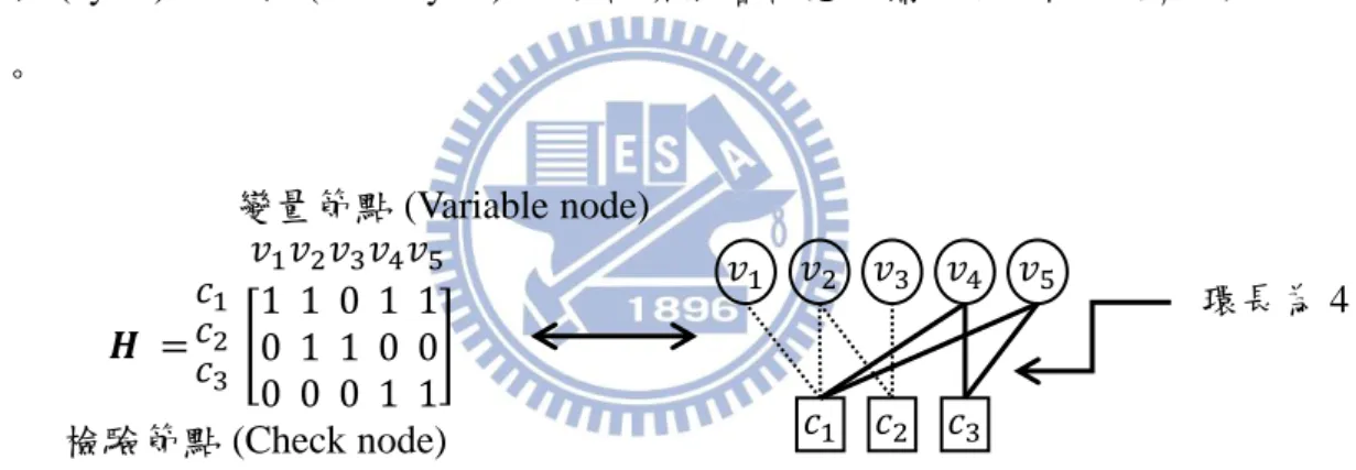
圖 1 檢驗矩陣與 Tanner graph 的關係 ... 1 圖 2 通訊系統架構示意圖... 3 圖 3 ACE 示意圖 ... 4 圖 4 (𝑎, 𝑏) trapping set 示意圖 ... 4 圖 5 LDPC codes process ... 5圖 6 Degree distribution of check nodes... 8
圖 7 不同方法效能圖... 9
圖 8 不同方法效能趨勢示意圖... 9
圖 9 Structurally equivalent and Regularly equivalent ... 10
圖 10 Bipartite graph 與 Unipartite graph 的轉換 ... 11
圖 11 Neighborhood connectivity illustration ... 12
圖 12 Neighborhood connectivity 比較圖 ... 13
圖 13 Random 與 PEG-based 不同 degree 的 Average shortest path length... 14
圖 14 不同方法所有節點的 average shortest path length ... 14
圖 15 Betweeness Centrality illustration ... 15
圖 16 Random 與 PEG-based 不同 degree 的 Betweeness centrality . 16 圖 17 不同方法所有節點的 betweeness centrality ... 16
圖 18 Degree Spectrum illustration ... 18
圖 19 Random, PEG-based average degree spectrum distribution ... 22
圖 20 不同方法的 role model 分類 ... 24
圖 21 Topology by MCL ... 28
圖 22 Average shortest path length of PEG-based cluster ... 30
圖 23 Betweeness centrality of PEG-based cluster ... 31
圖 24 Cluster histogram by MCL ... 31 圖 25 MCL cluster 範例圖 ... 32 圖 26 MCL intra-cluster 範例圖 ... 32 圖 27 MCL intra-cluster 𝑎 = 2 範例圖 ... 32 圖 28 MCL inter-cluster 範例圖 ... 33 圖 29 MCL in-out-cluster 範例圖 ... 34 圖 30 MCL out-cluster 範例圖 ... 34 圖 31 PEG MCL trapping 𝑎 = 2 比較結果 ... 35 圖 32 IPEG MCL trapping 𝑎 = 2 比較結果 ... 35 圖 33 MIPEG MCL trapping 𝑎 = 2 比較結果 ... 35 圖 34 PEG MCL trapping 𝑎 = 3 比較結果 ... 36 圖 35 IPEG MCL trapping 𝑎 = 3 比較結果 ... 36 圖 36 MIPEG MCL trapping 𝑎 = 3 比較結果 ... 37
圖 37 The betweeness centrality in clusters of PEG ... 38
圖 38 The betweeness centrality in clusters of IPEG... 38
圖 39 The betweeness centrality in clusters of MIPEG ... 38
圖 41 Cluster histogram by Modularity ... 41
圖 42 Average shortest path length of each cluster ... 42
圖 43 Betweeness centrality of each cluster ... 43
圖 44 Modularity cluster 範例圖 ... 44
圖 45 Modularity intra-cluster 範例圖 ... 44
圖 46 Modularity inter-cluster 範例圖 ... 44
圖 47 Modularity in-out-cluster 範例圖 ... 45
圖 48 Modularity out-cluster 範例圖 ... 45
圖 49 PEG Modularity trapping set 𝑎 = 2 比較結果 ... 45
圖 50 IPEG Modularity trapping set 𝑎 = 2 比較結果 ... 46
圖 51 MIPEG Modularity trapping set 𝑎 = 2 比較結果 ... 46
圖 52 PEG Modularity trapping set 𝑎 = 3 比較結果 ... 47
圖 53 IPEG Modularity trapping set 𝑎 = 3 比較結果 ... 47
表目錄
表 1 Progress-edge-growth algorithm ... 6
表 2 Modified-Improved PEG (MIPEG) algorithm... 7
表 3 Degree distribution of variable nodes ... 8
表 4 QC-LDPC codes ... 8
表 5 Distance illustration ... 19
表 6 Pattern and distance of PEG-based with check node degree=8 ... 21
表 7 Markov cluster algorithm ... 26
表 8 Markov cluster algorithm example ... 26
表 9 Markov cluster algorithm parameter setting ... 27
表 10 大 cluster 內 node 原始的 degree distribution ... 29
一.
緒論
1.1.
研究背景與動機
低密度奇偶檢查碼 (Low-density parity check code, LDPC code) 是一種用於
更正傳輸過程中發生錯誤的編碼方式,具有好的錯誤校正能力。低密度奇偶檢查
碼可以透過奇偶檢驗矩陣 (parity-check matrix,𝑯) 表示,奇偶檢驗矩陣由變量節
點 (variable node) 與檢驗節點 (check node) 構成,奇偶檢驗矩陣能夠利用
Tanner graph 圖形化表示,讓我們更清楚了解低密度奇偶檢查碼的結構。奇偶檢 驗矩陣與 Tanner graph 的關係如圖 1 所示,而 Tanner graph 中不可避免的存在
著環 (cycle),短環 (short cycle) 已被證實影響訊息傳播的獨立性降低解碼效
能。
圖 1 檢驗矩陣與 Tanner graph 的關係
Progressive edge- growth (PEG) algorithm [1] 是一種簡單且可避免構成短環 用來建構有限長度之低密度奇偶檢查碼的方法,許多其他演算法 [2] [3] 都是基
於 PEG 演算法加以改善來提升解碼效能。然而針對 Tanner graph 中除了短環
降低解碼效能之外,是否還存在其他結構上的因素影響解碼效能目前還是開放性 問題。 𝑯 = 環長為 4 變量節點 (Variable node) 檢驗節點 (Check node)
1.2.
研究方法
建構低密度奇偶檢查碼的方法 [4] [5] 提到了複雜網路理論 (Complex network theory) 在建構低密度竒偶檢查碼時的關聯性,文中利用複雜網路理論所 提到的 scale-free network [6] 網路結構特徵,來建構低密度奇偶檢查碼,讓低密 度奇偶檢查碼的節點符合 scale-free network 的節點特性,來提升解碼效能。 針對低密度奇偶檢查碼的結構,我們使用分群演算法將節點分群,利用馬可夫分群演算法 (Markov Cluster Algorithm) [7] 與模組性分群演算法 (Modularity
cluster algorithm) [8] 將結構性強的節點分在同一群中,找出影響 error floor
region 的結構,並且利用網路參數 (network parameter) 觀察不同群的節點特性, 解釋與解碼效能相關的群的特性與網路參數。
1.3.
論文架構
本文第二章將簡介低密度奇偶檢查碼與影響效能的因素,並且概述本文所觀 察的低密度奇偶檢查碼的結構所使用的建構方法,同時介紹社群模組與低密度奇 偶檢查碼的關聯;第三章將探討並觀察 Tanner graph 結構中節點的特性,本文 稱為 “宏觀” 分析低密度竒偶檢查碼的結構;第四章將透過不同的分類方法找出 子結構,本文稱為 “局部” 分析低密度竒偶檢查碼的結構,並且觀察子結構與效 能的關係;第五章將總結影響低密度竒偶檢查碼結構上的因素,與未來可深入討 論的方向。二.
背景知識
2.1.
簡介低密度奇偶檢查碼
低密度奇偶檢查碼 (Low-density parity check code, LDPC code) [9] [10]是一
種用來更正傳輸過程中發生錯誤的編碼方式。如圖 2 資料傳送先經過編碼器 (encoder),經過編碼器後傳出來的資料除了原始資料還多了一些多餘的資料 (redundant-bits),使得裡面的資料具有數學結構,當經過通道後不論是原始資料 或多餘的資料都有可能發生錯誤,但是因為資料存在著數學結構,所以解碼器 (decoder) 就能夠透過原有的數學結構將錯誤更正,這就是錯誤更正碼的基本概 念 [11]。低密度奇偶檢查碼的解碼演算法主要使用和積演算法 (Sum-Product
Algorithm),透過 Tanner graph 能夠更清楚了解解碼過程。
圖 2 通訊系統架構示意圖
以下為常見的影響低密度奇偶檢查碼效能的因素:
(1) Girth(shortest cycle length) 是表示所有 cycle 裡面 cycle length 最短的
length,cycle 的存在使得某一節點所送出的訊息經過 cycle 又回到自己, 而破壞了訊息的獨立性,使得和積演算法無法計算正確的事後機率,影
響解碼在 waterfall region 的效能。
(2) ACE 定義為 ∑𝑗(𝑑𝑠𝑗− 2),𝑠𝑗 為 variable node,𝑑𝑠𝑗 表示 𝑠𝑗 variable
node 的 degree 數,ACE 值計算 cycle 上 variable node degree 減 2 的
degree 數總和,圖 3 為 ACE 值計算方式示意圖,圖中環上有 3 個
check node,3 個 variable node,而每一個 variable node degree 減掉 2 Encoder data Channel Decoder data redundancy good
data noisy data
後得到的 ACE 值為 7,ACE 值越大表示有更高的機會能夠將迴圈上的
錯誤拯救回來,提高錯誤訊息被更正的機率。
圖 3 ACE 示意圖
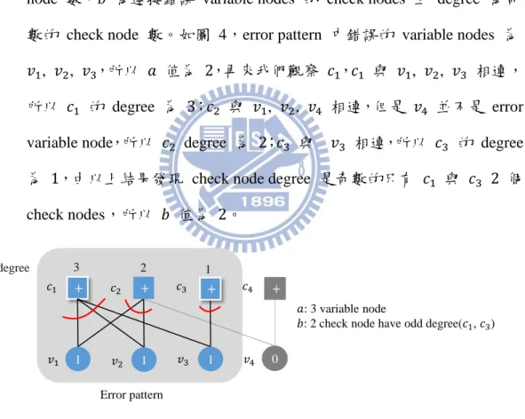
(3) (𝑎, 𝑏) trapping set [12] 影響 error floor region,𝑎 為發生錯誤的 variable
node 數,𝑏 為連接錯誤 variable nodes 的 check nodes 且 degree 為奇
數的 check node 數。如圖 4,error pattern 中錯誤的 variable nodes 為
, , ,所以 𝑎 值為 2,再來我們觀察 , 與 , , 相連,
所以 的 degree 為 3; 與 , , 相連,但是 並不是 error
variable node,所以 degree 為 2; 與 相連,所以 的 degree
為 ,由以上結果發現 check node degree 是奇數的只有 與 2 個
check nodes,所以 𝑏 值為 2。
圖 4 (𝑎, 𝑏) trapping set 示意圖
𝑎 越小表示越少 variable node 發生錯誤,所以發生機率越高,而 𝑏 值表示
能被多少個 check nodes 偵測到錯誤,當 𝑏 值越小表示被偵測的機會越小,所
以 (𝑎, 𝑏) 值越小所形成 trapping set 錯誤率越高,而本文將透過計算 (𝑎, 𝑏)
trapping set 的計算方式,評估挑選 variable node 形成錯誤率高的 trapping set 的機率。
ACE = 7
Variable node Check node
𝑎: 3 variable node
𝑏: 2 check node have odd degree( , )
1
Error pattern
degree 2 1
1 1 0
2.1.1.
建構低密度奇偶檢查碼演算法的分類
建構低密度奇偶檢查碼時從 Tanner graph 的角度來看,是給定 1 組
variable node degree distribution,variable node 依序選擇 check node 相連,如圖
5,假設目前 tanner graph 已經長到左圖,右圖 variable node 選擇 check node
連接,不同的方法選擇不同的 check nodes 連接。
圖 5 LDPC codes process
我們觀察的低密度奇偶檢查碼 variable node 數約 1000,check node 數約
500,利用以下的方法建構,我們將所使用的方法分類,以下依序介紹:
Random
這一類的 LDPC codes 是最原始的選擇方式,沒有加入改善的機制。
Random
在建構低密度奇偶檢查碼時 “任意選擇” check node 連接,導致產生的
check node degree 分布是 normal distribution,並沒有特別集中在某些 值。
Check nodes Variable nodes
Zigzag
建構低密度奇偶檢查碼時,優先選擇沒有連接過的 check node 連接。
PEG-based
建構低密度奇偶檢查碼時不可避免會產生迴圈 (cycle),PEG 演算法主要目
的是拉長迴圈長度 (cycle length) 來提高解碼效能,這一類的 LDPC codes 是基
於 PEG 加以改善建構方法。
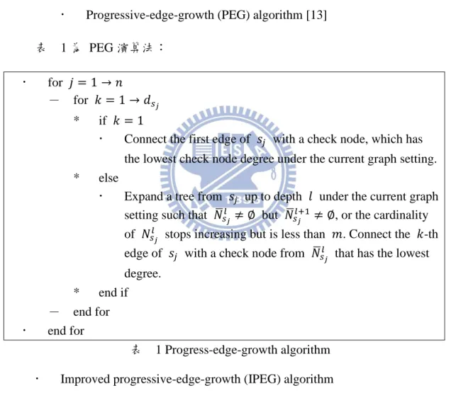
Progressive-edge-growth (PEG) algorithm [13] 表 1 為 PEG 演算法:
for 𝑗 = → 𝑛 - for 𝑘 = → 𝑑𝑠𝑗
* if 𝑘 =
Connect the first edge of 𝑠𝑗 with a check node, which has the lowest check node degree under the current graph setting. * else
Expand a tree from 𝑠𝑗 up to depth 𝑙 under the current graph setting such that 𝑁̅𝑠𝑗𝑙 ≠ ∅ but 𝑁̅𝑠𝑗𝑙+ ≠ ∅, or the cardinality of 𝑁𝑠𝑗𝑙 stops increasing but is less than 𝑚. Connect the 𝑘-th edge of 𝑠𝑗 with a check node from 𝑁̅𝑠𝑗𝑙 that has the lowest degree.
* end if - end for end for
表 1 Progress-edge-growth algorithm
Improved progressive-edge-growth (IPEG) algorithm
基於 PEG 演算法, [2] 提出了 ACE (approximated cycle extrinsic message
degree) 的概念,建構低密度奇偶檢查時不只拉長 cycle length 還加入 ACE 值,
ACE 定義為 ∑𝑗(𝑑𝑠𝑗− 2),計算迴圈 variable node 的 degree 減掉 2, ACE 值
越大表示迴圈上的 variable node 有更多機會透過其他不在迴圈上的邊 (edge)
Modified Improved PEG (MIPEG) algorithm
[13] 結合了 PEG 與 IPEG,在效能上優於 PEG 與 MIPEG,表 2 為
MIPEG [13]演算法:
for 𝑢 = → 𝑤
- for each 𝑠𝑗 ∈ 𝑆𝑢 (First Edge Connection)
* Find the subset of 𝐶 of check nodes, which has the lowest check node degree under the current graph setting. Among the subset 𝐶, the check node candidate of the first edge which can create the largest cycle length on its second edge is chosen.
- end for
- while at least one variable nodes not reaches its degree
* For each 𝑠𝑗 ∈ 𝑆𝑢 whose degree is smaller than 𝑑𝑠𝑗, expand a tree from 𝑠𝑗 up to depth 𝑙 under the current graph setting such that
𝑁𝑠𝑗
̅̅̅̅𝑙 ≠ ∅ but 𝑁̅̅̅̅𝑠𝑗𝑙+ = ∅, or cardinality of 𝑁𝑠 𝑗
𝑙 stops increasing
but is less than 𝑚.
* Let 𝑉 a set of comprising the variable nodes that have the largest depth 𝑙𝑚𝑎𝑥 among all tree expansions.
* Let 𝑅 be a subset of 𝑉, which can form cycles with the largest cycle ACE.
* Let Ω𝑗 be a subset of check nodes that consists of the check
nodes in 𝑁̅̅̅̅𝑠𝑗𝑙𝑚𝑎𝑥 and has the lowest degree.
* Randomly choose a variable node 𝑠𝑖 𝜖 𝑅. The check node in Ω𝑖 that can make the new forming cycles have the largest cycle ACE is selected.
- end end for
表 2 Modified-Improved PEG (MIPEG) algorithm
上述五種演算法在建造碼的時候皆已避免產生環長為 4 (short cycle
length=4) 的情況,都是使用相同長度與相同 variable node degree distribution 如 表 3 所建構,variable node 數為 1008,check node 數為 504,圖 6 為建構後
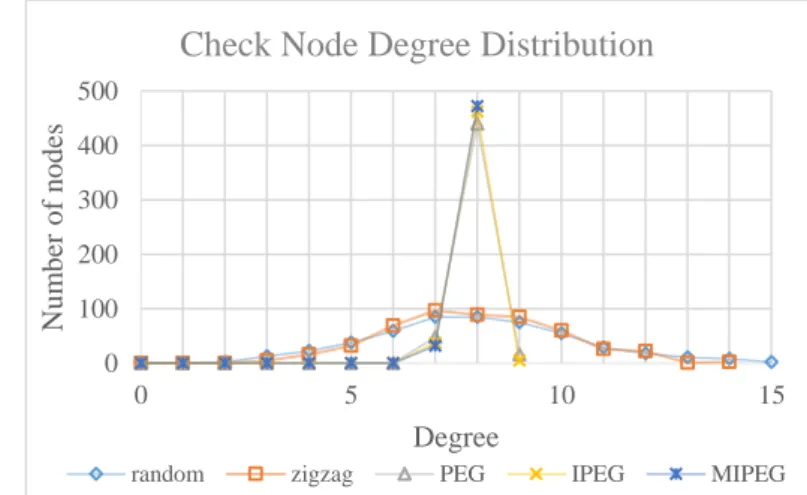
check node degree distribution,可以發現 PEG-based 的 check node degree 只會 集中在 7~9,而 Random 的分布像 normal distribution。
Degree Nodes 2 480 3 282 4 36 5 110 15 100 表 3 Degree distribution of variable nodes
圖 6 Degree distribution of check nodes
QC-LDPC codes
QC-LDPC codes 是 regular LDPC codes,variable node degree 與 check node
degree 都只有一種,表 4 為我們所建構的 QC-LDPC codes 的資訊。
QC-LDPC codes
Number of variable node 1038
Number of check node 519
The degree of variable node 3
The degree of check node 6
表 4 QC-LDPC codes 0 100 200 300 400 500 0 5 10 15 Nu m b er o f n o d es Degree
Check Node Degree Distribution
圖 7 不同方法效能圖
圖 8 不同方法效能趨勢示意圖
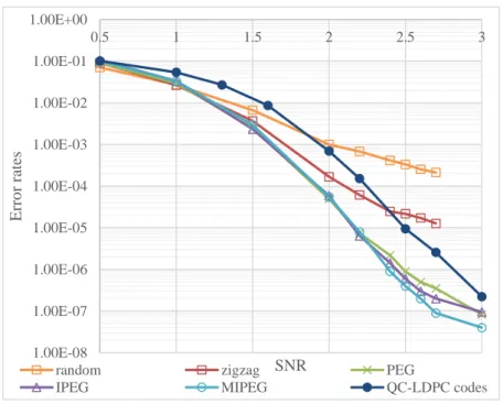
圖 7 為上述建構方法效能模擬的表現,圖 8 為效能趨勢示意圖,由圖 8 可
以發現在 waterfall region 的部分,Error rates 由大到小為 QC-LDPC codes >
Random > PEG-based,Error rates 越大表示錯誤率越高效能越差,PEG-based 效 能最好,再來是 random,表現較差的是 QC-LDPC codes;而在 error floor region
的部分 Error rates 由大到小為 Random > PEG-based > QC-LDPC codes,QC-LDPC
codes 表現最好,再來是 PEG-based,而 Random 在 error floor 表現最差。
1.00E-08 1.00E-07 1.00E-06 1.00E-05 1.00E-04 1.00E-03 1.00E-02 1.00E-01 1.00E+00 0.5 1 1.5 2 2.5 3 E rr o r rates SNR
random zigzag PEG
IPEG MIPEG QC-LDPC codes
QC-LDPC codes
PEG-based
Waterfall region
Error floor region SNR
Erro
r
rates
2.2.
社群模組 (Community/Block models)
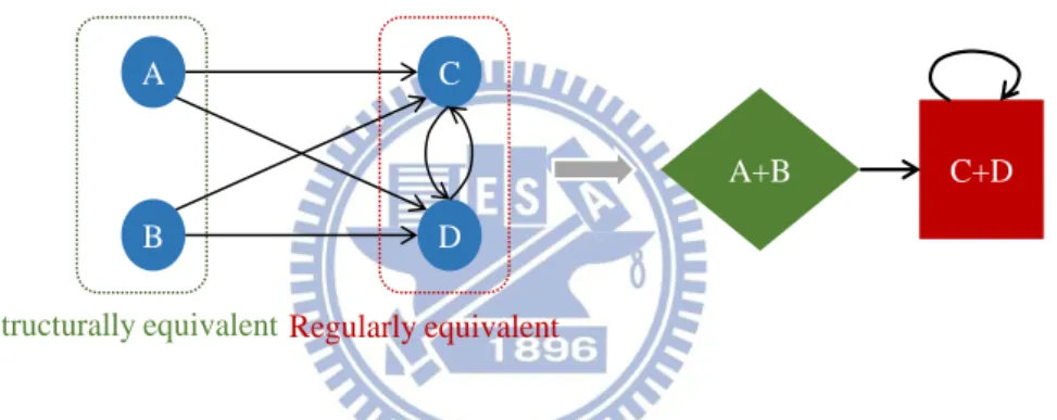
透過分群的方法會將存在 equivalent 關係的節點分在同一個Community/Block 中,而 equivalent 又分為 Structurally equivalent 與 Regularly
equivalent;如果兩個節點的鄰近節點都相同,那就表示這兩個節點是 Structurally
equivalent,如圖 9 中 node A 與 node B 都連接 node C 與 node D,所以
node A 與 node B 是 structurally equivalent 的關係;而 node C 與 node D 被 相同 equivalent 的 node A 與 node B 相連,且 node C 連接到 node D,而 node
D 連接到 node C,節點連接到相同 equivalent 的節點稱為 regularly
equivalent。
圖 9 Structurally equivalent and Regularly equivalent
本文使用 “局部” (Mesoscopic) 觀察來表示利用不同的分類方法分析
LDPC codes,分類方法為:角色模組 (role model)、馬可夫分群演算法 (Markov
Cluster algorithm)、模組性 (Modularity),其中 role model 為 regularly equivalent 的分類方法,Markov Cluster algorithm 與 Modularity cluster algorithm 為
structurally equivalent 的分類方法,本文第四章將詳細說明其演算法與分析結 果。 C+D A+B A B D C Regularly equivalent Structurally equivalent
三.
宏觀 (Macroscopic) 分析低密度奇偶
檢查碼結構
我們使用 2.1.1 所提到的各種演算法 (Random, zigzag, PEG, IPEG, MIPEG,
QC-LDPC codes) 建構出來的 Tanner graph 進行以下的分析,找出不同類型的演
算法影響效能的結構差異。
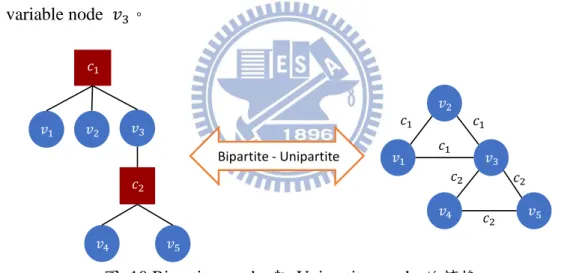
Tanner graph 是二分圖 (bipartite graph),variable node 只會與 check node 連接,透過簡單的轉換能夠將 bipartite graph 轉換成 unipartite graph,如圖 10
將 bipartite graph 轉換成 variable node 的 unipartite graph,unipartite graph 上的
每一條 edge 表示 check node,例如 variable node 透過 check node 可走
到 variable node 。
圖 10 Bipartite graph 與 Unipartite graph 的轉換
LDPC codes 解碼過程中 variable node 的訊息傳遞影響解碼效能,所以我們 觀察 variable node 的 unipartite graph,將 Tanner graph 轉換成只有 variable
node 與 variable node 連接的 unipartite graph,找出 variable node 到 variable
node 的 unipartite graph 中,是不是存在著影響 variable node 訊息傳遞的因 素。
3.1.
網路參數 (Network Parameters)
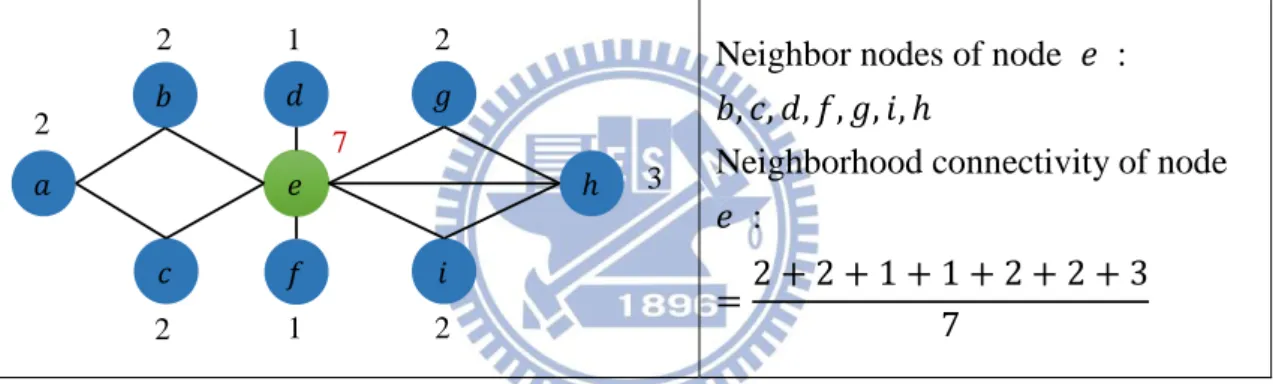
網路理論中存在許多參數來表現網路結構特徵,我們先將網路參數進行分類 與說明參數的表現意義,再來將網路參數與低密度奇偶檢查碼的關聯性加以描述, 最後針對低密度奇偶檢查碼不同方法的參數分析結果進行討論。 與鄰近節點 (neighborhood) 相關的參數 1. Neighborhood connectivityConnectivity 代表節點的度 (degree),Neighborhood connectivity 計算鄰近節 點 degree 的平均值,圖 11 計算 node 𝑒 的 Neighborhood connectivity。
Neighbor nodes of node 𝑒 : 𝑏, , 𝑑, 𝑓, 𝑔, 𝑖, ℎ
Neighborhood connectivity of node 𝑒 :
=2 2 2 2 3 7
圖 11 Neighborhood connectivity illustration
我們是計算 variable node 的 neighborhood connectivity,而 variable node 只
與 check node 連接,所以觀察 variable nodes 的 neighborhood connectivity 與
check node degree distribution 有關,圖 12 為不同方法的 neighborhood
connectivity,由圖可以發現效能差的碼,例如 random, zigzag,Neighborhood
connectivity 值較不一致,效能好的碼,例如 PEG, IPEG, MIPEG,Neighborhood
connectivity 值較一致,QC-LDPC codes 的 variable node 與 check node 的
degree 都只有一個值,並不適合使用 neighborhood connectivity 觀察。
𝑑 𝑏 𝑎 ℎ 𝑓 𝑒 𝑖 𝑔 2 2 2 2 2 1 1 3 7
圖 12 Neighborhood connectivity 比較圖
與最短路徑 (shortest path) 相關的參數
LDPC codes 解碼效能與 variable node 的訊息傳遞距離有關,所以接下來有 關最短路徑參數本文使用 variable node 的 unipartite graph 分析,並統計不同
degree 下的分布情形,找出不同 degree 中的差異。
1. Average shortest path length 是計算節點到其他節點的最短路徑。
The average shortest path length of node 𝑛: ∑ 𝐿(𝑛, 𝑖) 𝑁− 𝑁
𝑖= , 𝑖≠𝑛 (1)
𝐿(𝑛, 𝑚): The length of shortest path between node 𝑛 and 𝑚. 𝑁 : all nodes in graph.
7.5 8 8.5 9 9.5 2 3 4 5 15 Av er ag e Neig h b o rh o o d C o n n ec tiv ity
variable node degree
Neighborhood connectivity
圖 13 Random 與 PEG-based 不同 degree 的 Average shortest path length
由圖 13 可以發現,high degree variable node 的 shortest path length 較短,
high degree 在傳遞訊息比較容易將訊息傳遞給其他 node,所以 high degree 的
variable node 容易將自己的訊息傳送給其他 nodes。接下來觀察所有 node 的
average shortest path length,由圖 14 可以發現,不同方法所有 node 的 average
shortest path length 沒有差異,透過觀察所有節點的 shortest path 無法區分不同 建構方法。
圖 14 不同方法所有節點的 average shortest path length
1.80 2.00 2.20 2.40 2.60 2 3 4 5 15 Av er ag e Sh o rtest P ath L en g th
Variable node degree
Average Shortest Path Length Distribution
random zigzag PEG IPEG MIPEG
0.00 0.50 1.00 1.50 2.00 2.50 3.00
Average shortest path length
2. Betweeness centrality 是計算節點在最短路徑上的機率。 𝐶𝑏(𝑛) = ∑ (𝜎𝑠𝑡𝜎(𝑛) 𝑠𝑡 ) 𝑠≠𝑛≠𝑡 (𝑁 − 2 ) (2) 𝑠 : 𝑛𝑜𝑑𝑒 𝑠, 𝑡: 𝑛𝑜𝑑𝑒 𝑡
𝜎𝑠𝑡: node 𝑠 到 node 𝑡 的總 shortest path 數
𝜎𝑠𝑡(𝑛) : node 𝑠 到 node 𝑡 的 shortest path 且經過 𝑛 的 path 數 𝑁 : the number of nodes
圖 15 計算 node 𝑏 的 Betweeness centrality:
𝐶𝑏(𝑏) = ( (𝜎𝑎𝑐(𝑏) 𝜎𝑎𝑐 ) ( 𝜎𝑎𝑑(𝑏) 𝜎𝑎𝑑 ) (𝜎𝑎𝑒𝜎(𝑏) 𝑎𝑒 ) ( 𝜎𝑐𝑑(𝑏) 𝜎𝑐𝑑 ) (𝜎𝑐𝑒𝜎(𝑏) 𝑐𝑒 ) ( 𝜎𝑑𝑒(𝑏) 𝜎𝑑𝑒 ) ) 6 = ( ) ( ) ( 2 2) (2) ( ) ( ) 6 = 3.5 6 ≈ .583 All Shortest Path
𝑎 − 𝑎 − 𝑏 − / 𝑎 − 𝑑 𝑎 − 𝑏 − 𝑑 / 𝑎 − 𝑒 𝑎 − 𝑏 − − 𝑒 𝑎 − 𝑏 − 𝑑 − 𝑒 2/2 − 𝑑 − 𝑏 − 𝑑 − 𝑒 − 𝑑 /2 − 𝑒 − 𝑒 / 𝑑 − 𝑒 𝑑 − 𝑒 /
圖 15 Betweeness Centrality illustration
節點的 Betweeness centrality 值越大表示節點位在最短路徑上的機率越高, 也就表示圖中傳送訊息時容易經過 betweeness centrality 高的節點,那也就表示 這個節點自己的訊息容易被更改,不易形成 trapping set。 𝑒 𝑑 𝑏 𝑎
圖 16 Random 與 PEG-based 不同 degree 的 Betweeness centrality
由圖 16 可以發現 high degree variable node 的 betweeness centrality 值較
大,而我們知道 high degree variable node 不容易形成 trapping set,low degree
variable node 容易形成 trapping set,透過 betweeness centrality 的觀察發現相對 應的趨勢;接下來計算所有節點的 betweeness centrality,可以由圖 17 發現,不 同方法差異不大,無法透過所有節點的 betweeness centrality 區分不同建構方 法。 圖 17 不同方法所有節點的 betweeness centrality 1.00E-05 1.00E-04 1.00E-03 1.00E-02 1.00E-01 2 3 4 5 15 Av er ag e B etw ee n ess C en tr ality
Variable node's degree
Betweeness Centrality Distribution
random zigzag PEG IPEG MIPEG
0.00E+00 2.00E-04 4.00E-04 6.00E-04 8.00E-04 1.00E-03 1.20E-03 1.40E-03 1.60E-03 BetweennessCentrality Betweeness centrality
本節所使用的網路參數與 neighborhood 有關的 neighborhood connectivity
可以用來觀察 node degree distribution,不同方法建構的 check node degree
distribution 不同,透過 neighborhood connectivity 可以觀察 degree distribution
的差異。與 shortest path length 有關的參數可以用來觀察節點傳遞訊息的距離,
低密度奇偶檢查碼的解碼過程與 variable node 傳遞訊息的路徑有關,可以透
過計算 variable 到 variable node 的 shortest path length 來觀察傳遞的情形;
3.2.
度譜 (Degree Spectrum)
[14] 提出度譜 (Degree Spectrum) 的概念,定義一個節點的鄰近節點
(neighbor node) 的 degree 稱為 degree spectrum,如圖 18 所示,check node
的 degree = 7,則 的 degree spectrum 為 2, 2, 3, 3, 4, 5, 15。文中觀察 check
node 的 degree spectrum,文中提到透過 PEG 演算法所建構出來的低密度奇偶
檢查碼 check node 的 degree spectrum 會集中在特定的 degree spectrum,且
degree spectrum 間相似,如果增加 degree spectrum 相異的程度就能夠提升解碼 效能。
圖 18 Degree Spectrum illustration
本文定義了樣式 (pattern) 與距離 (distance) 兩種參數,pattern 用來觀察
degree spectrum 的相異性,distance 用來觀察 degree spectrum 的相似程度。
QC-LDPC codes 的 variable node 與 check node 的 degree 只有一種,不適合用
degree spectrum 來觀察。
表 3 為我們所分析的低密度奇偶檢查碼演算法的 variable node degree
distribution,pattern 的定義為 (Check node’s degree; N(15) N(5) N(4) N(3) N(2)),
N(𝑛) 表示 degree=𝑛 的 variable node 個數。圖 18 check node 的 degree = 7,
degree spectrum 為 2, 2, 3, 3, 4, 5, 15,則我們用 pattern (7; 1 1 1 2 2) 來表示。
我們統計所有 check node 的 pattern 出現的頻率,以最高頻率出現的
pattern 為基準,計算其他 pattern 與最高頻率出現 pattern 的差值,定義為
distance,計算方式如表 5。
2 2 3 3 4 5 15
變量節點 (Variable node)
檢驗節點 (Check node) 變量節點的度 (degree)
Pattern 頻率 Distance (7; 2 1 1 1 2) 2 (𝟕; 𝟐 𝟏 𝟏 𝟐 𝟏) − (7; 2 2) = |7 − 7| |2 − 2| | − | | − | |2 − | | − 2| = 2 (7; 2 1 1 2 1) 10 最高頻率 pattern (7; 2 1 0 2 2) 7 (𝟕; 𝟐 𝟏 𝟏 𝟐 𝟏) − (7; 2 2 2) = |7 − 7| |2 − 2| | − | | − | |2 − 2| | − 2| = 2 (7; 1 0 2 2 2) 1 (𝟕; 𝟐 𝟏 𝟏 𝟐 𝟏) − (7; 2 2 2) = |7 − 7| |2 − | | − | | − 2| |2 − 2| | − 2| = 4 表 5 Distance illustration
利用不同演算法所建構出來的 check node degree 不同,圖 6 為不同方法產
生的 check node degree distribution,由圖中可以觀察到 Random 所產生出來的
check node degree distribution 較分散,類似 normal distribution,而 PEG-based 所 產生出來的 check node degree distribution 較集中,這是因為 PEG 演算法每次
選擇連接的 check node 時,優先選擇不造成短環的情況下 degree 最小的 check
node,所以選擇的過程幾乎都是 degree 最小的 check node 優先被選到,這就使 不同的 check node 最後的 degree 集中在特定的值;而 IPEG 與 MIPEG 都是
基於 PEG 改善,產生後的 check node degree 也都集中在特定的值。
由圖 6 可以發現 PEG-based 在 check node degree=8 的數量最多,我們選
擇 check node 來觀察每一個 check node 的 degree spectrum,利用 pattern 與
PEG Number Of Check Node: 440
n(15) n(5) n(4) n(3) n(2) Frequency Probability Distance
4 1 0 2 1 10 2.3% 2 4 1 0 1 2 2 0.5% 2 4 0 1 2 1 1 0.2% 4 4 0 1 1 2 3 0.7% 4 3 2 0 2 1 7 1.6% 2 3 2 0 1 2 9 2.0% 2 3 1 1 1 2 131 29.8% 2 3 1 0 2 2 260 59.1% 0 3 0 1 2 2 1 0.2% 2 2 2 0 2 2 16 3.6% 2
IPEG Number Of Check Node: 462
n(15) n(5) n(4) n(3) n(2) Frequency Probability Distance
4 0 1 1 2 5 1.1% 4 4 0 0 2 2 11 2.4% 2 3 2 0 2 1 8 1.7% 2 3 2 0 1 2 41 8.9% 2 3 1 1 2 1 8 1.7% 2 3 1 1 1 2 116 25.1% 2 3 1 0 3 1 1 0.2% 2 3 1 0 2 2 265 57.4% 0 3 0 0 3 2 1 0.2% 2 2 2 0 2 2 6 1.3% 2
MIPEG Number Of Check Node: 472
n(15) n(5) n(4) n(3) n(2) Frequency Probability Distance
4 1 0 2 1 2 0.4% 2 4 1 0 1 2 2 0.4% 2 4 0 1 2 1 3 0.6% 4 4 0 1 1 2 14 3.0% 4 4 0 0 3 1 3 0.6% 4 4 0 0 2 2 12 2.5% 2 3 2 0 2 1 11 2.3% 2 3 2 0 1 2 52 11.0% 2 3 1 1 2 1 14 3.0% 2
3 1 1 1 2 97 20.6% 2 3 1 0 3 1 9 1.9% 2 3 1 0 2 2 227 48.1% 0 3 0 2 1 2 1 0.2% 4 3 0 0 3 2 7 1.5% 2 2 3 0 2 1 1 0.2% 4 2 3 0 1 2 2 0.4% 4 2 2 1 1 2 4 0.8% 4 2 2 0 2 2 11 2.3% 2
表 6 Pattern and distance of PEG-based with check node degree=8
表 6 列出 PEG, IPEG, MIPEG 的 check node degree 為 8 的 pattern 與
distance,PEG 的 pattern 數是 10 組,distance 差異為 2 的有 7 組,差異為 4
的有 2 組,表示 pattern 間與最高頻率發生的 pattern 相似,PEG 的 degree
spectrum 相似;IPEG 的 pattern 數是 10 組,distance 差異為 2 的有 8 組,
差異為 4 的有 1 組,表示 pattern 間與最高頻率發生的 pattern 相似,IPEG 的
degree spectrum 相似;而 MIPEG 的 pattern 數是 18 組,distance 差異為 2 的
有 10 組,差異為 4 的有 7 組,相較於 PEG 與 IPEG,MIPEG 的 pattern 間
與最高頻率發生的 pattern 不相似,MIPEG 的 degree spectrum 不相似,驗證了
[14] 所提出的觀察。
透過 degree spectrum 的觀察,Random 沒有集中的 pattern,pattern 種類多;
PEG-based pattern 種類不多,與建構後的 check node degree 有關,degree
spectrum 集中在特定的 pattern,且 distance 差異大,pattern 間相似程度小。
當沒有集中在特定 pattern 時,我們使用以下將介紹的平均度譜 (Average
Degree spectrum) 來觀察。
平均度譜 (Average Degree Spectrum) 為 degree spectrum 的平均值,如圖
用 average degree spectrum 來觀察不同演算法所建構的低密度竒偶檢查碼的
average degree spectrum 分布,觀察不同建構方法的分布情形。
圖 19 Random, PEG-based average degree spectrum distribution
Random 分布是常態分布 (normal distribution),PEG-based 的 average
degree spectrum 值集中在 7 到 8.5 之間,表示 PEG-based 產生的 average
degree spectrum 相似度高,皆集中在某些值。
由以上的結果發現 degree spectrum 與建構後的 check node degree
distribution 有關,效能好的碼 check node degree 集中在某些值,degree spectrum 也集中,degree spectrum 間與高頻率發生的 degree spectrum 越不相似效能更好;
效能差的碼 check node degree 分散,沒有高頻率發生的 degree spectrum,我們
也驗證了 [14] 所提出的結論,透過本文提供 pattern 與 distance 的表示方式, 能更方便的觀察 degree spectrum。 0 50 100 150 200 250 300 3 3.5 4 4.5 5 5.5 6 6.5 7 7.5 8 8.5 9 9.5 10 10.5 11 11.5 12 12.5 13 13.5 14 14.5 15 n u m b er o f p att ern
Average Degree Spectrum
Average Degree Spectrum Distribution
四.
局部 (Mesoscopic) 分析低密度奇偶檢
查碼結構
此章節我們將利用不同的分類方式將低密度奇偶檢查碼的節點分類,同一類 的節點具有一些相似的特性,透過分類的結果我們觀察每一類中的節點特性,找 出不同類中節點的差異,並觀察是否存在影響解碼效能的因素。 以下介紹我們所使用的分類方法,以及將低密度奇偶檢查碼的節點分類後的 結果與討論。4.1.
角色模組 (Role model)
角色模組 (Role model ) 是一種 Regularly equivalent 的分類方法,我們使用
Jörg Reichardt [15] [16] 提供的 Role model for complex network [17] 分析方法將 低密度奇偶檢查碼分類,設定分成 5 種 role,圖 20 中每一個單位是 1 個 role,
左側藍色圓圈 role 中都是 variable nodes,右側紅色方框 role 中都是 check
nodes。 random zigzag 356 257 337 315 247 1026 985 40 965 947 37 372 253 320 316 251 1029 945 40 998 955 33
PEG IPEG
MIPEG
圖 20 不同方法的 role model 分類
由圖 20,不同方法分類後藍色 role 中 variable nodes 數量分布平均,紅色
role 中 check nodes 數量分布平均,role 間的連線每一個方法差不多,無法觀察 到不同建構方法的差異。
透過實驗的結果發現 role model 這種 regularly equivalent 分類方法將低密
度機偶檢查碼區分為 variable node 與 check node 兩類,而 variable node 本來
就只會跟 check node 連線,透過 regularly equivalent 並無法區分不同建構方法
的連線方式,所以 regularly equivalent 這種分類方式並不適合將低密度奇偶檢查 碼的節點進行分類。 390 253 377 241 251 67 1366 560 1389 544 74 353 265 330 325 239 1193 846 48 62 1057 794 396 257 313 299 247 1023 984 37 1004 907 45
4.2.
馬可夫分群演算法 (Markov Cluster
Algorithm)
Markov Cluster Algorithm (MCL) 是屬於 structurally equivalent 的分類方法, 由 Stijn van Dongen [7] 提出,是一種能夠將大量節點分群 (cluster) 的方法,
MCL 已應用在分析複雜生物網路,例如蛋白質交互作用的網路拓撲
(Topological Similarity of Protein Interaction Network),透過 MCL 進行 protein
family detection;還有人類的疾病基因研究 (Disease-Gene network),人類的疾病 基因網路 (Disease-Gene network) 是一種二分圖 (bipartite graph),利用 MCL 可
以預測疾病基因網路,分群後的結果表示同 cluster 內的基因容易透過生物反映
程序作用影響同 cluster 內的疾病,相較於任意選擇的基因,同 cluster 內的基
因有比較大的機率影響同 cluster 內的疾病。
MCL 是一種基於隨機漫步 (random walk) 的方法來不斷模擬節點在圖中行 走的路徑,經過一段時間後,節點在某個區域內行走的機率較高,這些區域稱為
群 (cluster)。MCL 主要的兩種運算是 expansion 和 inflation,expansion 的目的
主要是讓節點能夠在不同節點間行走,inflation 的目的主要是放大每一條線
(edge) 行走的機率,透過初始的 stochastic matrix 不斷的執行 expansion 和
inflation 將節點分群 (cluster)。表 7 為 MCL 的演算法。
Step 1. Input a Graph, expansion parameter 𝑒, inflation parameter 𝑟; Step 2. Create the adjacency matrix from the graph;
Step 3. Add self-loops;
Step 4. Normalize the matrix 𝑀;
Step 5. Expand the matrix with 𝑒𝑡ℎ power, i.e. (𝑀)𝑒;
Step 6. Inflate by taking inflation of the resulting matrix with parameter 𝑟; Step 7. Repeat step 5 and step 6 until a steady state is achieved;
Definition: [18]
Given a matrix 𝑀 ∈ ℛ𝑘×𝑙, 𝑀 ≥ , and a real nonnegative number 𝑟,
the matrix resulting from rescaling each of the columns of 𝑀 with power coefficient 𝑟 i
s called 𝛤𝑟𝑀, and 𝛤𝑟 is called the inflation operator with power coefficient 𝑟. Formall
y, the action of 𝛤𝑟: ℛ𝑘×𝑙 → ℛ𝑘×𝑙 is defined by
(𝛤𝑟𝑀)𝑝𝑞 = (𝑀𝑝𝑞) 𝑟 / ∑(𝑀𝑖𝑞) 𝑟 𝑘 𝑖=
表 7 Markov cluster algorithm
expansion parameter = 2, inflation parameter = 2 Step 1 ( ) ( ) 𝑀 = ( /3 /3 /3 /3 /3 /3 /4 /4 /4 /4 /4 /4 /4 /4 /3 /3 /3 /3 /3 /3)
Step 2 Step 3 Step 4
𝑀 = ( .3 .3 .3 . 8 .3 .3 .3 . 8 .23 .23 .29 . 3 . 6 . 6 . 6 . 6 . 3 .29 .23 .23 . 8 .3 .3 .3 . 8 .3 .3 .3 ) 𝛤𝑀 = ( .33 .33 .33 . 2 .33 .33 .33 . 2 .25 .25 .4 . 7 . 2 . 2 . 2 . 2 . 7 .3 .25 .25 . 2 .33 .33 .33 . 2 .33 .33 .33) Step 5 Step 6 Step 8
表 8 Markov cluster algorithm example
表 8 為 Markov cluster algorithm 範例圖,經過 MCL 運算後節點 1, 2, 3
分在同一個 cluster,節點 4, 5, 6 分在同一個 cluster。 1 2 3 4 5 6 1 2 3 4 5 6
我們所分析的低密度奇偶檢查碼的 Tanner graph 就是 bipartite graph,且節
點數多,適合利用 MCL 將低密度奇偶檢查碼進行分群。本文使用 Cytoscapse
[19] 一種用於分析複雜網路分析的平台來分析,其中提供許多插件用於分析複
雜網路,例如 clusterMaker [20],clusterMaker 提供了 MCL 這種分群演算法,
表 9 為 MCL 參數設定,藉由 MCL 的分析後,不同方法的群結構分布如圖
21,MCL 會將 bipartite graph 切割出許多不同大小的 cluster,圖 24 統計不同 大小的 cluster 數量。
MCL Parameter Value Expansion parameter 2 Inflation parameter 2 Number of iteration 16 表 9 Markov cluster algorithm parameter setting
PEG topology IPEG topology
QC-LDPC codes topology
Check node Red color
Variable node Blue color
Largest cluster MIPEG topology
圖 21 Topology by MCL
由圖 21 發現 PEG-based 的碼透過 MCL 的分群後,都存在著 1 個大的
度分布 (Degree distribution)
由馬可夫分群演算法 (Markov Cluster Algorithm) 的分析我們發現 high
degree 的 variable node 不屬於任何 cluster,cluster 內的 variable node 都是
low degree variable node,表 10 為 PEG-based 最大群內 variable node 與 check
node 原本的 degree distribution。
number of variable nodes
Degree PEG IPEG MIPEG
2 307 331 306
3 201 210 172
5 54 65 55
total nodes 562 606 533
number of check nodes
Degree PEG IPEG MIPEG
7 4
8 260 264 223
total nodes 264 264 223
表 10 大 cluster 內 node 原始的 degree distribution
MCL 將 high degree variable node 作為 isolated node 不屬於任何 cluster,
這是因為 MCL inflation 的步驟,high degree 的分母較大,透過不斷的疊代後,
high degree node 上的 edge 走的機率就趨近於 0。
網路參數 (Network Parameter)
我們利用網路參數觀察每一個 cluster 內有關 variable node 到 variable
node 與最短路徑相關的參數,比較 PEG-based 中不同的方法 PEG, IPEG,
MIPEG 的差異,由圖 7 知道 PEG > IPEG > MIPEG,MIPEG 表現最好,透過
以下的分析本文找到了反映效能趨勢的網路參數。
1. Average shortest path length
圖 22 為 PEG-based cluster 在不同 degree 下 average shortest path length
的表現,由結果可以發現,不同 degree 下 MIPEG 的 average shortest path length
皆比 IPEG 和 PEG 長,由 Tanner graph 的觀點,希望 cycle length 越長越好,
如果在設計低密度奇偶檢查碼時考量 variable node 到 variable 的 shortest path
length,增加 shortest path length 或許也能增加 cycle length 的長度。MCL 切出 的大 cluster,所有節點的 average shortest path length 影響 waterfall region 的效
能。
圖 22 Average shortest path length of PEG-based cluster
2. Betweeness centrality
由圖 23 的結果可以發現,MIPEG 的 betweeness centrality 都比其他方法
值較大,也就表示 MIPEG 不同 degree 下的 variable node 成為 trapping set 的
機率比其他方法低。在設計低密度奇偶檢查碼時考慮節點的 betweeness centrality
或許能夠避免節點成為 trapping set,提升 error floor region 的效能。 y = 0.0352x2- 0.3043x + 4.4196 R² = 1 y = 0.0389x2- 0.3148x + 4.4856 R² = 1 y = 0.0107x2- 0.2666x + 5.2311 R² = 1 3.8 4 4.2 4.4 4.6 4.8 5 2 3 5 av er ag e sh o rtest p ath len g th degree
Average Shortest Path Length Distribution
PEG IPEG MIPEG
圖 23 Betweeness centrality of PEG-based cluster
圖 24 Cluster histogram by MCL
由圖 21 與圖 24 發現 QC-LDPC codes 本身是一個大的 cluster,而
PEG-based 的部分擁有一個比較大的 cluster,cluster size 約 1000,但也有一些 小的 cluster,而 Random 的部分都是由小的 clusters 組成,表現了 Random,
PEG-based 與 QC-LDPC codes 的 error floor region 的效能趨勢如圖 7,小
clusters 數量越多,錯誤率越高,我們猜測是不是這些小的 clusters 造成 trapping set 導致 error floor region 的表現不佳,所以我們討論小 clusters 中 (𝑎, 𝑏)
trapping set 的分布情形。 y = 0.002x2- 0.002x + 0.0027 R² = 1 y = 0.0003x2+ 0.0032x - 0.0007 R² = 1 y = 0.0007x2+ 0.0053x - 0.0029 R² = 1 0.002 0.02 2 3 5 av er ag e b etw ee n ess ce n tr ality degree
Betweeness Centrality Distribution
PEG IPEG MIPEG
多項式(PEG) 多項式(IPEG) 多項式(MIPEG)
1024, 1 1024, 1 1024, 1 2048, 1 0 20 40 60 80 100 120 140 160 2 4 8 16 32 64 128 256 512 1024 2048 Nu m b er o f clu ster s Cluster Size Cluster Histogram
random zigzag PEG IPEG MIPEG QC-LDPC codes
QC-LDPC codes
PEG-based Largest cluster
由 2.1.1 我們知道 𝑎 值越小發生機率越高,𝑏 值越小錯誤機率越大,本文
比較以下 4 種情況下比較 (𝑎, 𝑏) trapping set 發生機率:
假設透過 MCL 分析後,cluster 分布如圖 25。
圖 25 MCL cluster 範例圖
1. intra-cluster : 同一個小 cluster 內選 (𝑎, 𝑏) trapping set 如圖 26。
圖 26 MCL intra-cluster 範例圖
假設在每一個小 cluster 內選 2 個 variable node,如圖 27,選到的 𝑏 值 分布如表 11:
圖 27 MCL intra-cluster 𝑎 = 2 範例圖
小 cluster
Number of variable nodes : 14
Red nodes : check nodes Blue nodes : variable nodes
out_cluster 小 cluster 5 𝑎 5 𝑎 2 𝑎 2 𝑎 小 cluster 5 2 5 2 2 2 2 2 = 22
b Cluster1 Cluster 2 Cluster 3 Cluster 4 Ratio 2 4 5 1 1 22= .5 3 3 3 6 22= .27 4 3 2 5 22= .23 表 11 MCL intra-cluster 𝑎 = 2, 𝑏 分布表
綠底的部分表示在 Cluster1 選 2 個 variable node,(𝑎, 𝑏) = (2, 2) 的組合
數有 4 個;而在 intra-cluster 內任選 2 個 variable node (𝑎, 𝑏) = (2, 2) 的組合
數就是把 𝑏 = 2 那一列相加,總共有 11 個;接下來 normalize 所有小 cluster
內任選 2 個 variable nodes 的組合數,總共是 22 個,所以
就表示在 intra-cluster 內任選 2 個 variable node (𝑎, 𝑏) = (2, 2) 比例 (Ratio) 為 .5 ,利
用這種計算方式表示 intra-cluster 內任選 𝑎 個 variable node 的比例分布。
2. inter-cluster : 屬於小 cluster 的 node 選 (𝑎, 𝑏) trapping set 如圖 28,
normalize 的分母為 ( 4 𝑎)。
圖 28 MCL inter-cluster 範例圖
小 cluster
Number of variable nodes : 14
4 𝑎
3. in-out-cluster : 小 cluster 內選 個 node,out-cluster 內任選 𝑎 −
個 nodes,如圖 29,normalize 的分母為 ( 4) × ( 𝑁 𝑎 − )。
圖 29 MCL in-out-cluster 範例圖
4. out-cluster : out-cluster 內選 (𝑎, 𝑏) trapping set 如圖 30,normalize 的
分母為 (𝑁
𝑎)。
圖 30 MCL out-cluster 範例圖
本文以下比較 PEG, IPEG, MIPEG 上述的 4 種情況挑選 (𝑎, 𝑏) trapping set
的 ratio。
小 cluster
Number of variable nodes : 14
Red nodes : check nodes Blue nodes : variable nodes
out_cluster
4
𝑁 𝑎 −
Number of variable nodes: 𝑁
𝑁
𝑎 out_cluster
圖 31 PEG MCL trapping (𝑎 = 2) 比較結果
圖 32 IPEG MCL trapping (𝑎 = 2) 比較結果
由圖 31、圖 32、圖 33 可以發現,𝑎 = 2 intra-cluster 挑選到 (𝑎, 𝑏) trapping set 的機率最大。 圖 34 PEG MCL trapping (𝑎 = 3) 比較結果 圖 35 IPEG MCL trapping (𝑎 = 3) 比較結果
圖 36 MIPEG MCL trapping (𝑎 = 3) 比較結果
由圖 34、圖 35、圖 36 可以發現 𝑎 = 3 時 intra-cluster 挑選到 (𝑎, 𝑏)
trapping set 的機率也是最大。
透過以上的結果發現在小 cluster 內確實容易挑到 (𝑎, 𝑏) trapping set。我們
一開始提到 trapping set 與 betweeness centrality 的關係,接下來我們統計小
clusters 內 nodes 的 betweeness centrality 如圖 39 發現小 clusters 內 nodes 的 betweeness centrality 都比較小,而 high degree node 的 betweeness centrality
比其他節點高出許多,圖最右邊紅色表示 high degree node 的 betweeness
圖 37 The betweeness centrality in clusters of PEG
圖 38 The betweeness centrality in clusters of IPEG
圖 39 The betweeness centrality in clusters of MIPEG
0.00E+00 2.00E-03 4.00E-03 6.00E-03 8.00E-03 1.00E-02 1.20E-02 0.00E+00 1.00E-04 2.00E-04 3.00E-04 4.00E-04 5.00E-04 6.00E-04 12 9 8 6 5 4 3 2 high b etwe en es s ce n tra lity cluster size
PEG
0.00E+00 2.00E-03 4.00E-03 6.00E-03 8.00E-03 1.00E-02 1.20E-02 0.00E+00 1.00E-04 2.00E-04 3.00E-04 4.00E-04 5.00E-04 6.00E-04 18 10 7 6 5 4 3 2 high b etwe en es s ce n tra lity cluster sizeIPEG
0.00E+00 2.00E-03 4.00E-03 6.00E-03 8.00E-03 1.00E-02 1.20E-02 0.00E+00 1.00E-04 2.00E-04 3.00E-04 4.00E-04 5.00E-04 6.00E-04 20 13 12 10 9 7 6 5 4 3 2 high b etwe en es s ce n tra lity cluster sizeMIPEG
由本節的實驗結果可以發現 LDPC codes 的 Tanner graph 透過 MCL 的分
群後,QC-LDPC codes 只有一個 cluster,表示不容易受到其他節點突發狀況而
影響,也反映了 QC-LDPC codes 在 error floor region 表現較好的趨勢;而
Random 則是有許多小 clusters,表示 Random 的 LDPC codes 容易受到突發狀 況影響,也反映了 Random 表現都比其他方法差的趨勢;而 PEG-based 透過
MCL 的分群後,具有 1 個較大的 cluster 和少許的小 clusters,表示 PEG-based 中的大 cluster 內部救回錯誤節點的機會較高,透過 network parameter 的分析
也反映了 MIPEG 參數值 (average shortest path length, betweeness centrality) 都
大於其他方法;另外在小 cluster 的部分,透過比較 intra-cluster, inter-cluster,
in-out-cluster 與 out-cluster,我們發現 intra-cluster 最容易選到 (𝑎, 𝑏) trapping
4.3.
模組性 (Modularity)
Modularity 是一種網路結構性質,由 M.E.J Newman 提出 [8] [21],用來衡 量網路在分割後的結構品質,表示分割後每一個子結構中連線較緊密,但子結構 間只有少數的連線。Modularity 的定義如下: 𝑀𝑜𝑑𝑢𝑙𝑎𝑟𝑖𝑡𝑦 𝑄 = 2𝑚∑ [𝐴𝑣𝑤− 𝑘𝑣𝑘𝑤 2𝑚 ] 𝛿( 𝑣, 𝑤) 𝑣𝑤 (3)
𝑚: ∑𝑣𝑤𝐴𝑣𝑤 is the number of edges in graph
𝐴𝑣𝑤= { if vertices and 𝑤 are connected otherwise 𝑘𝑣: the degree of vertex
Vertex belong to community 𝑣 𝛿(𝑖, 𝑗) is if 𝑖 = 𝑗 and otherwise
先假設每一個 node 屬於不同的 cluster,挑選能夠增加 Modularity 值的
node 加入同一個 cluster,直到無法增加 Modularity 值後完成此次 cluster 的挑 選;接下來選擇其他 node 依序再次選擇能夠增加 Modularity 值的 node 加入
同一個 cluster,依序不斷挑選。
由 (3) 可以發現 Modularity 是與隨機網路的連線情況比較,連線比隨機網
路的連線越緊密則表示分割的結果越好,每一個子結構內的連線緊密,表示 node
彼此間傳遞訊息需要經過的 path 較短,在 LDPC codes decoding 的情況下,越
近的越容易將錯誤更正,所以發生錯誤時 cluster 內的 node 能夠互相幫忙更正,
cluster 越大,有越多 nodes 能夠幫忙,cluster 越小則表示幫忙更正的 nodes 數 少,所以我們利用 Modularity 分割 variable node 的 unipartite graph。
本文使用 Cytoscapse [19] 的插件 clusterMaker [20] 提供的 Modularity 分
Random topology Zigzag topology
PEG topology IPEG topology
MIPEG topology
圖 40 Topology by Modularity
圖 41 Cluster histogram by Modularity
0 1 2 3 4 2 4 8 16 32 64 128 256 512 fre q u en cy cluster size
cluster histogram
由圖 40、圖 41 無法從 topology 與 cluster histogram 的觀點觀察出不同方
法的差異,接下來我們觀察每一個 cluster 內 network parameter (average shortest
path length, betweeness centrality) 的特性。
圖 42 Average shortest path length of each cluster
0 0.5 1 1.5 2 2.5 3 347 300 264 76 21 av era ge s h o rtes t p at h le n gth cluster size random 0 0.5 1 1.5 2 2.5 3 333 327 252 48 39 6 3 av era ge s h o rtes t p at h le n gth cluster size zigzag 0 0.5 1 1.5 2 2.5 3 448 420 128 8 4 av era ge s h o rtes t p at h le n gth cluster size PEG 0 0.5 1 1.5 2 2.5 3 393 373 169 55 18 av era ge s h o rtes t p at h le n gth cluster size IPEG 0 0.5 1 1.5 2 2.5 3 324 287 255 109 22 8 3 av era ge s h o rtes t p at h le n gth cluster size MIPEG
圖 43 Betweeness centrality of each cluster
如圖 42 所示由 average shortest path length 無法看出不同 cluster size 的
差異,但是透過圖 43 可以發現 cluster size 越小的 betweeness centrality 越小,
我們假設這些小 cluster 的 node 容易形成 trapping set,本文比較以下 4 種情
況下比較 (𝑎, 𝑏) trapping set 發生機率: 0.00E+00 5.00E-04 1.00E-03 1.50E-03 2.00E-03 347 300 264 76 21 b etwe en es s ce n tra lity cluster size Random 0.00E+00 5.00E-04 1.00E-03 1.50E-03 2.00E-03 333 327 252 48 39 6 3 b etwe en es s ce n tra lity cluster size Zigzag 0.00E+00 2.00E-04 4.00E-04 6.00E-04 8.00E-04 1.00E-03 1.20E-03 1.40E-03 1.60E-03 448 420 128 8 4 b etwe en es s ce n tra lity cluster size PEG 0.00E+00 5.00E-04 1.00E-03 1.50E-03 2.00E-03 393 373 169 55 18 b etwe en es s ce n tra lity cluster size IPEG 0.00E+00 2.00E-04 4.00E-04 6.00E-04 8.00E-04 1.00E-03 1.20E-03 1.40E-03 1.60E-03 324 287 255 109 22 8 3 b etwe en es s ce n tra lity cluster size MIPEG
假設透過 Modularity 分析後,cluster 分布如圖 44。
圖 44 Modularity cluster 範例圖
1. intra-cluster : 同一個小 cluster 內選 (𝑎, 𝑏) trapping set 如圖 45,
normalize 的分母為 (4 𝑎) × (
3 𝑎)。
圖 45 Modularity intra-cluster 範例圖
2. inter-cluster : 小 cluster 選 (𝑎, 𝑏) trapping set 如圖 46,normalize 的分
母為 (7 𝑎)。
圖 46 Modularity inter-cluster 範例圖
小 cluster
Number of variable nodes : 7
out_cluster
Number of variable nodes : 𝑁
小 cluster
Number of variable nodes : 7
4 𝑎
3 𝑎
小 cluster
Number of variable nodes : 7
7 𝑎
3. in-out-cluster : 小 cluster 內選 1 個 node,out-cluster 內任選 𝑎 − 個 nodes,如圖 47,normalize 的分母為 (7 𝑎) × ( 𝑁 𝑎 − )。 圖 47 Modularity in-out-cluster 範例圖
4. out-cluster : out-cluster 內選 (𝑎, 𝑏) trapping set 如圖 48,normalize 的
分母為 (𝑁
𝑎)。
圖 48 Modularity out-cluster 範例圖
以下比較 PEG, IPEG, MIPEG 上述的 4 種情況選 (𝑎, 𝑏) trapping set 的
ratio。
圖 49 PEG Modularity trapping set (𝑎 = 2) 比較結果
小 cluster
Number of variable nodes : 7
out_cluster
Number of variable nodes : 𝑁
7 𝑁
𝑎 −
out_cluster
Number of variable nodes : 𝑁
𝑁 𝑎
圖 50 IPEG Modularity trapping set (𝑎 = 2) 比較結果
圖 51 MIPEG Modularity trapping set (𝑎 = 2) 比較結果
由圖 49、圖 50、圖 51 可以發現 𝑎 = 2 時 intra-cluster 挑選到 (𝑎, 𝑏)
圖 52 PEG Modularity trapping set (𝑎 = 3) 比較結果
圖 53 IPEG Modularity trapping set (𝑎 = 3) 比較結果
圖 54 MIPEG Modularity trapping set (𝑎 = 3) 比較結果
由圖 52、圖 53、圖 54 可以發現 𝑎 = 3 時 intra-cluster 挑選到 (𝑎, 𝑏)
trapping set 的機率最大。
由本節 Modularity 觀察 variable node unipartite graph 的結果可以發現,透
過 Modularity 的分群後,小 cluster 內的 variable node 的 betweeness centrality
較小,且透過比較 intra-cluster, inter-cluster, in-out cluster 與 out-cluster 可以發
現 intra-cluster 選到 (𝑎, 𝑏) trapping set 的機率最高,也證實了小 cluster 內確實
五.
結論
5.1.
研究成果
本文的研究問題是找出與效能有關的結構因素,透過實驗結果本文以下歸納
與效能相關的結構特性:
Markov cluster algorithm 與 Modularity 分群後小 clusters 數量越多,error
floor region 的錯誤率越大,所以小 cluster 容易形成 (𝑎, 𝑏) trapping set,而且小
cluster 內的 betweeness centrality 都比其他 node 小,所以 betweeness centrality 越小 error floor region 的效能越差。
在 waterfall region 表現好的碼,透過 Markov cluster algorithm 分群後具有
1 個大 cluster,大 cluster 結構中的 average shortest path length 較大。
5.2.
未來展望
不同的分類方式能夠聚集的節點特性不同,本文嘗試了 Markov Chain
Cluster Algorithm 與 Modularity 這兩種分群演算法後,發現了 clustering
algorithm 與 LDPC codes 間的關聯性。
還有許多其他 clustering algorithm 用於不同領域與不同網路結構的分析,哪
參考文獻
[1] X. Y. Hu, E. Eleftheriou, and D. M. Arnold, "Regular and irregular progressive edge-growth Tanner graphs," IEEE Trans. Inf. Theory, pp. 386-398, Jan 2005. [2] H. Xiao and A. H. Banihashemi, "Improved progressive-edge-growth (PEG)
construction of irregular LDPC codes," IEEE Comm. Letts., pp. 715-717, Dec 2004.
[3] S. M. v. Dongen, "Network analysis," [Online]. Available: http://micans.org/mcl/index.html?sec_mcledge.
[4] Francis C.M. LAU, Chi K. TSE and Zhiliang ZHU, "Future Design of Channel Codes: A Complex Network Perspective," Fourth International Workshop on
Chaos-Fractals Theories and Applications, pp. 156-160, 2011.
[5] X. Zhen, F.C.M Lau, C.K. Tse, Y. He, S. Hau, "Application of complex-network theories to the design of short-length low-density-parity check codes," IET
Communication, pp. 1569-1577, 2009.
[6] ALBERT-U\SZLOBARABASIANDERICBONABEAU, “Scale-Free Networks,” SCIENTIFIC AMERICAN, pp. 50-59, May 2003.
[7] S. v. Dongen, "Graph clustering by flow simulation," University of Utrecht, May 2000. [Online]. Available:
http://www.library.uu.nl/digiarchief/dip/diss/1895620/inhoud.htm.
[8] Aaron Clauset, M. E. J. Newman, and Cristopher Moore, "Finding community structure in very large networks," pp. 1-6, 30 Aug 2004.
[9] R. G. Gallager, in Low-Density Parity-Check Codes, 1963. [10] "Low-density parity-check code," [Online].
[11] 趙啟超, "錯誤更正碼簡介," [Online]. Available:
http://w3.math.sinica.edu.tw/math_media/d184/18404.pdf. [12] "Publications," [Online]. Available:
http://www2.engr.arizona.edu/~vasiclab/Projects/CodingTheory/ErrorFloorPubl ications.html.
[13] J.-D. Du, "Performance Improvement of PEG-based Construction for Finite-Length LDPC Codes," 2012.
[14] F.C.M. Lau W.M. Tam C.K. Tse, "Increasing the local girth of irregular low-density parity-check codes based on degree-spectrum analysis," IET
Communications, p. 1506–1511, May 2011.
[15] J. Reichardt. [Online]. Available:
http://intersci.ss.uci.edu/wiki/pub/JR/clustertoolmanual.pdf. [16] J. Reichardt, "Jörg Reichardt," [Online]. Available:
http://theorie.physik.uni-wuerzburg.de/~reichardt/index.html.
[17] J. Reichardt, and D.R. White, "Role models for complex network," THE
EUROPEAN PHYSICAL JOURNAL B, pp. 217-224.
[18] K. Macropol, "Clustering on Graphs: The Markov Cluster Algorithm (MCL)," 2009. [Online]. Available:
2.pdf.
[19] "Cytoscape," [Online]. Available: http://www.cytoscape.org/.
[20] "clusterMaker: Creating and Visualizing Cytoscape Clusters," [Online]. Available: http://www.cgl.ucsf.edu/cytoscape/cluster/clusterMaker.html.
[21] M. E. J. Newman and M. Girvan, "Finding and evaluating community structure in networks," Phys. Rev. E 69, pp. 1-16, August 2003.
[22] F. R. Kschischang, B. J. Frey and H. A. Loeliger, "Factor Graphs and the Sum-Product Algorithm," IEEE TRANSACTIONS ON INFORMATION
THEORY, VOL. 47, NO. 2, p. 498–519, FEBRUARY 2001.
[23] Rodolfo Baggio, Noel Scott, Chris Cooper, Network Science – A review focused
on tourism.
[24] J. D. a. S. Horvath, "Understanding network concepts in modules," BMC
Systems Biology 2007, 1:24 doi:10.1186/1752-0509-1-24, pp. 1-2, 4 June 2007.
[25] Yassen Assenov (Max Planck Institute for Informatics), Mario Albrecht (Max Planck Institute for Informatics), Mike Smoot (University of California, San Diego), "NetworkAnalyzer Online Help," Dec 2010. [Online]. Available: http://med.bioinf.mpi-inf.mpg.de/netanalyzer/help/2.7/.