國 立 交 通 大 學
電信工程研究所
碩 士 論 文
應用於多重拜占庭開放線段缺陷上以整數線性
規劃為基礎的錯誤診斷方法設計
Integer-Linear-Programming (ILP) Based
Diagnosis of Multiple Byzantine
Open-Segment Defects
研究生:高振源
指導教授:溫宏斌 教授
應用於多重拜占庭開放線段缺陷上以整數線性規劃為基礎的
錯誤診斷方法設計
Integer-Linear-Programming (ILP) Based Diagnosis of
Multiple Byzantine Open-Segment Defects
研 究 生:高振源 Student:Chen-Yuan Kao
指導教授:溫宏斌 Advisor:Hung-Ping Wen
國 立 交 通 大 學
電 信 工 程 研 究 所
碩 士 論 文
A ThesisSubmitted to Institute of Communication Engineering College of Electrical Engineering and Computer Science
National Chiao Tung University in partial Fulfillment of the Requirements
for the Degree of Master
in
Communication Engineering
July 2010
Hsinchu, Taiwan, Republic of China
i
應
用
於
多
重
拜
占
庭
開
放
線
段
缺
陷
上
以
整 數 線 性 規 劃 為 基 礎 的 錯 誤 診 斷 方 法 設 計
學生:高振源
指導教授
:溫宏斌 教授
國立交通大學電信工程研究所碩士班
摘
要
開放線段缺陷所表現的錯誤決定於拜占庭效應和實體電路的繞線情形。
拜占庭效應使得錯誤表現會依據模組和實體電路的資訊而變化,所以傳統
的自動模組產生器在確保缺陷錯誤的啟動與傳遞上顯得相當困難。這篇論
文提供了三階段的診斷方法設計用於自動尋找開放線段的組合。路徑回溯
技巧幫助我們從錯誤模組中擷取所有可能存在開放線段的位置。整數線性
規劃工具則根據可能的錯誤點和模擬結果列舉所有線路錯誤組合。最後,
錯誤模擬則刪除不符合的組合幫助我們找到實際符合錯誤效應的線段組
合。對 ISCAS85 電路注入多重開放線段缺陷的實驗結果顯示出此方法的分
辨率相當有效,且可以產生小於 9 組的診斷率高的錯誤組合。
ii
Integer-Linear-Programming (ILP) Based Diagnosis of Multiple Byzantine
Open-Segment Defects
student:Chen-Yuan Kao
Advisors:Dr. Hung-Ping Wen
Institute of Communication Engineering
National Chiao Tung University
ABSTRACT
The faulty responses of an open defect are determined by the Byzantine
effect and the physical routing. The Byzantine effect makes such faulty
behaviors non-deterministic and depends upon both the pattern and physical
information. Therefore, traditional ATPG has difficulty on its fault activation
and propagation. This paper proposes a three-stage diagnosis approach of
finding combinations of open-segment defects automatically. Path tracing
technique helps extract all candidate fault sites from error outputs of failing
patterns. An ILP solver enumerates all net fault by considering fault candidates
and simulation responses. Last, fault simulation identifies true open-segment
faults by pruning false cases. Experimental results shows the resolution of the
proposed approach is high and only generates <9 faults with good diagnosability
on all ISCAS 85 circuits under multiple injected open-segment defects.
iii
誌
謝
本論文得已完成,首先要先感謝這幾年來溫宏斌老師的細心教導,從老
師身上學到許許多多的事情,他也和我們分享知識上以及生活上的一切。
在我對研究方向迷失方向的時候,引領我的方向,指正我的錯誤。一路走
來即使艱辛,卻也因為有老師,才會如此甘之如飴。能成為老師的學生覺
得相當地慶幸,他所做的一切,對我的影響,良師益友正是相當貼切的形
容詞。未來在職場和研究的領域上,我會更加努力,不辜負老師的期望。
另外,還要感謝 CIA 實驗室的佳伶、韋廷、彥后、千慧、雨欣、家慶、
欣恬,這實驗室因為有你們變得熱鬧了起來,更加有活力。可以和你們在
學習和研究上互相切磋學習,相信我們都藉此成長了不少。同時還要感謝
VSLI 實驗室的焯基、懷中、宗祐,還有信龍,陪伴了我一開始的研究生涯,
在我最無依無靠的時候給予我支持和協助。最後要感謝一直鼓勵我,幫我
祈禱的翠芬姐、佩佩和其他朋友,由於你們的陪伴,我才能充實地完成這
碩士學業。
最後,將此論文謹獻給我的父母與家人。
Contents
List of Figures v
List of Tables vi
1 Introduction 1
2 Previous Researches 6
3 Fault Model of Open Segments 10
4 Three-Stage Integet-Linear-Programming (ILP) Based Diagnosis 14
4.1 Net Fault Identification . . . 16
4.2 N -net Fault Generation . . . 17
4.3 N -segment Fault Composition . . . 22
4.4 Performance Comparison of Applied Constraints . . . 23
5 Experimental Results 25 5.1 Results under Random Pattern . . . 27
5.2 Results under 5-detect Pattern . . . 27
5.3 Diagnosability and Resolution Comparison . . . 33
6 Conclusion 43
List of Figures
1.1 Two types of inter-gate open defects . . . 3
1.2 A net with three-fanout gate . . . 4
3.1 Fault model for an open defect . . . 11
3.2 Byzantine effect . . . 12
4.1 Three-stage ILP-based diagnosis flow . . . 15
4.2 An illustrative example for path tracing and weight assignment . . . 17
4.3 Path tracing of fault-propagation trees . . . 21
4.4 Two examples for X-inject-and-evaluate . . . 22
5.1 Net resolution . . . 39
5.2 Segment resolution . . . 40
5.3 Diagnosability . . . 41
5.4 Fault Detection According to Simulation Result . . . 42
List of Tables
4.1 Comparison of Applied Constraints for BIP Solving . . . 24
5.1 Circuit Information . . . 26
5.2 N =1 under 1000 random patterns . . . 28
5.3 N =2 under 1000 random patterns . . . 29
5.4 N =3 under 1000 random patterns . . . 30
5.5 N =4 under 1000 random patterns . . . 31
5.6 N =5 under 1000 random patterns . . . 32
5.7 5-Detect Stuck-at Pattern . . . 33
5.8 N =1 under 5-detect stuck-at patterns . . . 34
5.9 N =2 under 5-detect stuck-at patterns . . . 35
5.10 N =3 under 5-detect stuck-at patterns . . . 36
5.11 N =4 under 5-detect stuck-at patterns . . . 37
Chapter 1
Introduction
Failure analysis is critical for the yield improvement of manufacturing integrated cir-cuits (ICs) and collects and analyzes data to determine the cause of failures. In a typical failure analysis flow, diagnosis is the process of locating the possible faults as defects and these locations can be inspected on the silicon for further physical repair. However, along with the process technology advances, failure mechanisms such as electromigration and stress voiding result in intricate and dynamic faulty phenomena on ICs and jointly make deterministic fault models such as stuck-at faults no longer effective. Therefore, many advanced fault models arise to properly describe the underlying behaviors. Open defects, the unintended breaks or electrical discontinuities in interconnects, are one category of the most important production defects and become more vulnerable to the failure mechanisms for the deep submicron regime. Hence, the impact of failure mechanisms needs to be con-sidered during the diagnosis of open defects.
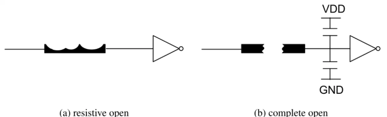
Open defects can be further classified into intra-gate opens and inter-gate opens. Intra-gate opens can be regarded as an open with an infinite resistance that disconnects the charge path or discharge path to the gate output whereas intra-gate opens are often re-garded as stuck-open faults. Inter-gate opens have significant influences on signal propa-gation through interconnects and can be further classified into two types: (1) resistive open and (2) complete open. Fig. 1.1 illustrates the two types of inter-gate open defects. Resis-tive opensare also known as weak opens under which the current still passes through the narrow open defects due to the tunneling effect. Complete opens, on the other hand, are often termed strong opens which make the driven gates of the net float. Hence, the voltage at the floating net is hard to predict. According to [6] [16], the majority of open defects are of the inter-gate type and a high percentage of the known open defects in metal lines belong to strong opens. Therefore, complete opens are the target defects studied in this paper.
Due to the lower power supply and closer wires in the deep submicron regime, parasitic capacitances have greater impact to circuits and induce more complicated circuit behav-iors. One of them is open segment where the faulty values on its downstream gates need to consider the impact of Byzantine effect [1] [2]. The Byzantine effect manifests Byzan-tine failures, in which components of a system fail in arbitrary ways. It denotes that the coupling of the neighboring nodes for a floating node determines its voltage value. and the logic values of its downstream gates are decided by comparing the current voltage with
VDD
GND
(a) resistive open (b) complete open
Figure 1.1: Two types of inter-gate open defects
respective threshold values. As result, the open-segment faults in the presence of Byzantine effect become dynamic failures and diagnosis of Byzantine open-segment faults requires the assistance of layout information and the cell library.
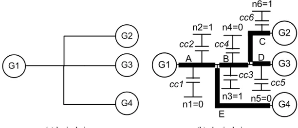
From a logical view, when a net that drives multiple gates is open, all of its downstream gates have faulty values. However, from a physical view, such a logical net can be further divided into multiple segments on the circuit layout where each segment can drive one or multiple gates. For example, gate G1 driving gate G2, G3 and G4 through a logical net is illustrated in Fig. 1.2(a). If an open occurs on the net and then a fault is generated, all downstream gates, G2, G3 and G4, receive faulty values. However, considering the physical routing as shown in Fig. 1.2(b), the net can be divided into five segments with six aggressors and their respective coupling capacitances. Segment A drives G2, G3 and G4. Segment B drives G2 and G3. Segment C drives G2. Segment D drives G3. Segment E drives G4. An open that occurs on different segments under different coupling conditions can result in different faulty behaviors. If the corresponding floating-node voltage is larger than the threshold value of the downstream gate, the input to the downstream gate receives logic 1. Otherwise, it receives logic 0. Last, the logic value on the driving gate decides if a faulty value is generated on the respective driven gate. To take Fig. 1.2(b) for example, if an open occurs on segment A and the coupling condition results in a floating-node voltage larger than the threshold voltages of G2 and G4 but smaller than that of G3, then G2, G3 and G4 will receive logic 1, logic 0 and logic 1, respectively. If G1 has logic 0, then the open on segment A generates two faults on G2 and G4.
G1 G2 G3 G4
n1=0
n2=1
n4=0
n3=1
n6=1
n5=0
cc1
cc2
cc4
cc3
cc5
cc6
G1
G2
G3
G4
A
B
E
D
C
(a) logical view (b) physical view
Figure 1.2: A net with three-fanout gate
Since different combinations of values on coupling nets result in different floating-node voltages, open-segment defects depend on physical information such as the layout and cell library and traditional physically-independent diagnosis cannot work well on this problem. Moreover, when multiple open defects occur physically, single-location-at-a-time (SLAT) patterns cannot differentiate the output responses under the single defect assumption from the ones under the multiple, simultaneously-active defect assumption. Therefore, our diag-nosis intends to fully utilize patterns and their output responses. The failing pattern set is first used to identify the possible segements that can cause the faulty output responses with open defects. Later, the passing pattern set takes a role of eliminating false candidates. On the basis of the idea, an integer-linear-programming(ILP) based approach is developed to formulate the relationship between patterns and responses and to further explore the seg-ment combinations as defects. Our objective of the proposed ILP based approach is to find segment combinations that have the fewest defects to precisely explain responses for all passing and failing patterns.
The rest of the paper is organized as follows. In Chapter 2, we will review the diagnosis and discuss different approaches of previous researches. The open-segment fault model will be elaborated in Chapter 3. Chapter 4 outlines the proposed three-stage ILP-based diagnosis flow and details the stage of fault-site identification, fault-combination
genera-tion and fault-simulagenera-tion validagenera-tion. Experimental results of applying the proposed flow are presented and cross compare the results of using the random and 5-detect patterns in Chapter 5. Conclusions and future work are discussed in Chapter 6.
Chapter 2
For interconnect open defects, many researches have been done about diagnosis and ATPG approach. To deal with the voltage prediction on the floating node, physical infor-mation and Byzantine effect estiinfor-mation are considered. To diagnose multiple open defects, several approaches are reviewed. Tranditional diagnosis approaches for multiple stuck-at faults cannot work well when undeterministic faulty behaviors by Byzantine effect appear. Different patterns may induce different faulty behaviors. Therefore, several approaches for diagnosing multiple defects without assuming a fault model are proposed. Finally, we will also discuss some diagnomsis approaches focus on multiple open defects.
Shi-Yu Huang proposes a single open-segment fault diagnosis approach [1] [20]. Can-didates are collected from sturctural analysis. Wei Zou et al. also propose a diagnosis approach for interconnect open defect considering routing topology and coupling capaci-tance to estimate Byzantine effect [2]. Both works use the inject-and-evaluate paradigm for open defects since their faulty behavior are not consistent. S. M. Reddy et al. proposes a gate-level fault model for interconnect opens whose number grows exponentially in terms of the fanout size [27]. They consider primary output information, and apply implicit enu-meration of faults and explicit fault simulation to decrease the number of fault that need to be considered.
Several other researches are denoted to test generation for interconnect open defects. S. Spinner et al. propose an algorithm to generate test patterns for an open defect consid-ering physical information and Byzantine effect [14]. They apply an aggressor selection to force the signals on aggressors for fault activation and verify the existence of a pattern for fault propagation. X. Lin et al. discuss all test generation strategy for all types of open defects [10]. S. Hillbert et al. use segment stuck-at faults to generate test patterns for inter-connect open defects [26]. In addition, untestability analysis is applied to identify which faults are not testable.
Multiple-defect diagnosis of failing ICs is more important along with the ever increas-ing number of gates and density of the circuits. Multiple open-segment fault diagnosis is more complex since two faults may have crosstalk with each other. When the faulty be-havior due to a open defect is determined by its neighboring nodes, its neighboring node may also affected by another open defect. Single open-segment fault diagnosis sometimes has a problem to describe a circuit under such circumstance. It is required to design a new
approach to diagnose multiple open segment defects.
T. Bartenstein et al. propose an approach to diagnose multiple stuck-at faults. SLAT patterns assumes that only one defect occurs on one single location at one time. By observ-ing simulation of SLAT patterns, multiplets are collected as the potential faults. In [5] [19] SLAT patterns are also used to facilitate diagnose multiple faults. However, SLAT patterns needs to perform equivalent fault evaluation that is also hard for open-segment defects. SLAT patterns can no longer guarantee the activation of the faulty behavior and the propa-gation for each defect. Furthermore, faulty behaviors of open-segment defects vary under different patterns. Z. Wang et al. explore the relationships between patterns and diag-nosability [25]. They use a ATPG tool to generate patterns for stuck-at fault. Their results reveals that the diagnosability is improved by providing patterns of better quality. However, n-detect patterns has not yet been explored on open-segment defects. We will conduct the experiments to observe the diagnosability of oepn-segment defect between random pattern and n-detect pattern.
X. Wen et al. [9] propose a diagnosis approach for physical defects with unnown behav-iors on logic level. They use a X-fault model for diagnosis via X-injection and simulation. Yu and Blanton propose a multiple defect diagnosis without a fault model by only observing failing pattern characteristics [3]. Path-based site elimination helps to reduce the number of candidate sites. J. Brandon Liu et al. propose an incremental diagnosis of multiple open interconnects [8]. A list of fault tuples is found to explain all EPOs after X’s are injected on candidate sites and implication is performed. However, for open-segment faults, the implication is inaccurate on nets whose some fanouts have faulty value while others have correct value due to Byzantine effect. R. Rodriguez-Montanes et al. used a logic-based diagnosis tool (Faloc) to diagnose open defect [24]. Then they presented a ranking based on the quiescent current consumption of the circuit under test.
Open segments are often modeled as interconnect open defects [2] [8] [12] [14] be-cause interconnects are the most convenient locations to be open. However, those diagno-sis approaches focus on either single defect assumption [1] [2] [20] or work at only logic level [8] [9] [12] [18]. Therefore, in this work, we propose a new approach which con-siders the Byzantine effect for diagnosing multiple open-segment defects.Since the faulty behavior due to multiple open-segment defects depends on both the input pattern and the
physical information, it is necessary to incorporate the circuit layout and the cell library in our approach.
Chapter 3
Several fault models of open defects has already been proposed in previous researches [2] [14] [22]. In this paper, we target the fault model that describes an open on one segment of the net considering the impact of physical information. When a segment of one net is open, the node f on the floating side is regarded as an open-segment fault. The logic value of the floating node f is determined by the floating node voltage and the threshold voltage of the driven gates. If the floating node voltage is larger than the threshold voltage of a driven gate, the logic value for the driven gate is logic 1; otherwise, it is logic 0. Therefore, not all driven gates of a floating node have faulty values.
Cn1 Cn0 Neighboring nodes (1) Neighboring nodes (0) open defect Cgnd Cvdd Vdd Gnd Ci1 Ci0 f
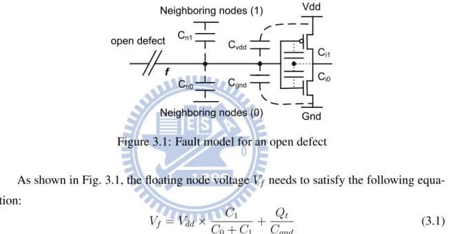
Figure 3.1: Fault model for an open defect
As shown in Fig. 3.1, the floating node voltage Vf needs to satisfy the following
equa-tion: Vf = Vdd× C1 C0 + C1 + Qt Cgnd (3.1)
where Qt is the initial trapped charge of the floating node and Cgnd is the capacitance
between floating node and ground. C0 and C1are the sum of the capacitances with logic 1
and logic 0, respectively. Furthermore, the values of C0 and C1can be decomposed into:
C0 = Cgnd+ Cn0+ Ci0 (3.2)
C1 = Cvdd+ Cn1+ Ci1 (3.3)
where Cvdd and Cgnd are the capacitances between the floating node and the power, and
between the floating and the ground, respectively. Cn0 and Cn1 are the capacitances
be-tween floating node and its neighboring node with logic 0 and logic 1, respectively. Ci0
Cn1 dominate the major part of fault behavior, we only observe the coupling effect from
Cn0and Cn1.
However, trapped charge Qtand internal capacitances, Ci0 and Ci1are typically hard
to predict. Process variation also makes parasitic capacitances extracted from physical layout unpredictable. Therefore, this paper adopts a simplified model similar to [10] [14] by assuming that the parasitic capacitances between the open net and its neighboring nets dominate the decision of the logic value on the floating node.
#1 open
G1
G2
G3
G4
#2 open
G1
G2
G3
G4
(a) (b)Figure 3.2: Byzantine effect
Given a floating node and its down-stream gates, if Vf > Vthreshold, the floating node f is
regarded as with logic 1. Otherwise, it is with logic 0. For example, in Fig. 3.2(a), suppose that Vt2, Vt3 and Vt4 are the threshold voltages for G2, G3 and G4, respectively. Assume
that Vt4 < Vt3 < Vf < Vt2, if segment #1 is open and, then G3 and G4 are logic-0 where
G2 is logic-1. If the segment #2 is open in Fig. 3.1(b) with the same voltage condition, G2 and G3 are logic-1 and logic-0, respectively, where G4 maintains the original correct value. For segment #1, the possible fault behavior is (G2, G3, G4), (G3, G4), and (G4) while for segment #2 is (G2, G3) and (G3). Therefore, different segments result in different fault behaviors. For an open-segment fault, the exact faulty behavior needs to consider the logic values of coupling wires.
Under the assumption of multiple faults in a circuit, if one open-segment fault is acti-vated under a pattern, the fault may become masked due to the logic value of its
neighbor-ing node is replaced by a faulty value. It is also possible that an inactive fault is activated by another fault. Fault masking effect is complicated and will be discussed in Section 5. Because the activation of an open defect requires specific assignments of signals on neigh-boring nets, fault equivalence needs a robust and rigorous definition in order to perform fault collapsing. Therefore, for simplicity, each open-segment fault is treated as an inde-pendent fault and has no equivalent fault. As result, the total number of open-segment faults is the number of segments of each net in the circuit.
Chapter 4
Three-Stage
Integet-Linear-Programming (ILP)
Based Diagnosis
Failing Pattern Pick Pattern i Path tracing from
EPO j More EPO?
More failing pattern?
BIP transformation under N defects
BIP solving Find solution?
Pick N-net fault k Update fault candidate weight
Net faults
Prune false open segments
Fault simulation with physical information Match output response? N-net faults True N-segment faults N e t fa u lt i d e n ti fi c a ti o n Yes No Yes No i++ j++ N -n e t fa u lt g e n e ra ti o n N -s e g m e n t fa u lt c o m p o s it io n Yes No N++ Yes k++ No Delete redundant constraints X inject and evaluate Match EPO response? No Yes Compose N-segment faults N-segment faults Pick N-segment fault m m++
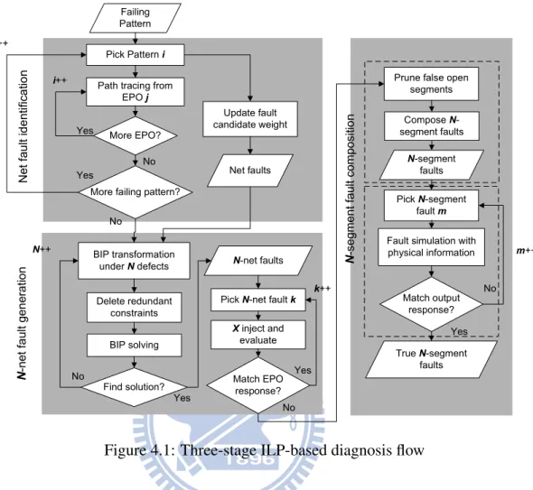
Figure 4.1: Three-stage ILP-based diagnosis flow
Having the open segment fault model, the next step is to find the set of faults that match the simulation results with respect to the given patterns. Therefore, a three-stage diagnosis approach is proposed to determine the number of faults and the corresponding segment combinations. Figure 4.1 shows the overall flow of the proposed approach that consists of three stages: the first one is net fault identification; the second one is N -net fault generation; the third one is N -segment fault composition. Net fault identification is developed based on typical logical filtering of candidate sites [1] [8] [18]. Then, by encoding the candidate nets as a binary-integer-programming (BIP) problem, a ILP solver incrementally finds net combinations as N -net faults where N starts from 1. If no net combination can be found to correctly explain the patterns expressed by the ILP constraints, N increments by 1 until a feasible solution is found. In the third stage, logical pruning by symbolic X simulation first reduces the size of N -segment faults. Later, the injection of
opens on segments with the support of physical information ensures that the remaining N -segment faults can result in the correct behaviors on the circuit under all patterns and thus requires further inspection on silicon.
4.1
Net Fault Identification
The first stage of the proposed diagnosis flow generates a list of candidate nets as faults. Each candidate in the list is called a net fault. The initial net-fault list is done by the path-tracing technique. Path path-tracing starts from an erroneous primary output (EPO) of one failing pattern. Nets are identified as defect locations and stored into a list of candidates during this stage. This process iterates to update the net-fault list for each EPO until failing patterns are fully explored.
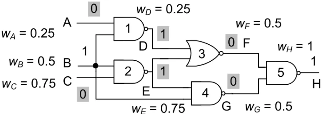
Backtracking algorithm runs for all failing patterns for path tracing. For each EPO, it traces the circuit backward to find the net on which an open can account for the output mismatch. If multiple fanins of a gate have controlling values, only those controlling fanin nets are considered and collected as net faults. If all fanins are non-controlling, all fanin nets are collected and the backtracking continues to run on each fanin net. Fig. 4.2 shows an example where the path tracing starts from net H. Considering the controlling values on both fanins of gate 5, net F and net G are net-fault candidates and stored in the list. For net G, both fanins are also collected because net B and net E have non-controlling values. For a net i, wi = 1 is labeled if an open occurring on net i can fully explain one EPO.
But if 0 < wi < 1 is labeled, an open on net i can partially explain one EPO. When path
tracing starts from one EPO, it is assigned the full weight 1. Given a specific weight w for the net connecting the output of a gate, if all inputs of the gate have non-controlling values (cv’s), all nets connecting its inputs are assigned weight w. When the gate has k simultaneous controlling-value inputs, the weight is split and each net connecting one input receives w/k. In summary, when a net receives multiple weight assignments from different branches, the total sum of all weights will be its final weight.
To give an example, a circuit under test is shown in Fig. 4.2 with the logic-value as-signments on all gates. Path tracing starts from net H with weight wH=1. Because both
1
D
2
E
3
F
1
w
D= 0.25
1
w
E= 0.75
4
G
5
H
0
0
1
A
w
F= 0.5
w
G= 0.5
w
H= 1
B
C
w
A= 0.25
w
B= 0.5
w
C= 0.75
0
0
1
Figure 4.2: An illustrative example for path tracing and weight assignment
net F and net G have controlling values to the gate connecting net H, wF = wG = 1/2 =
0.5. Similarly for net F , considering that both net D and net E have controlling values, wD = wE1 = wF/2 = 0.25. However, wE2 = wB = wG = 0.5 since both net E and net B
have non-controlling values to the gate connecting net G. Therefore, wE = wE1 + wE2 =
0.5+0.25 = 0.75. As a result, wA=0.25, wB=0.5, wC=0.75, wD=0.25, wE=0.75, wF=0.5,
wG=0.5 and wH=1.
4.2
N -net Fault Generation
The candidate list extracted from the first stage only collects the net-fault candidates la-beled with weights as the capability of correctly explaining EPOs under one failing pattern. In the second stage, we further explore the multiplets of net faults that can fully explain all EPOs under all failing patterns simultaneously. Note that a multiplet of k net faults is termed a N -net fault hereafter.
The weight assignment for each candidate now takes into play and transforms the search of combinations of net faults into a BIP problem. For example, given three EPOs under one failing pattern with the candidate list L1, L2 and L3 extracted from the first stage:
L1 = {A, B, C, E} for EP O1
L2 = {B, E} for EP O2
L3 = {A, D} for EP O3
To further decide the size N and the set of N -net faults that can fully explain all EPOs, the corresponding BIP problem can be expressed into:
nA+ nB+ nC+ nE ≥ 1
nB+ nE ≥ 1
nA+ nD ≥ 1
where all net variables, nA, nB, nC, nD and nE, are binary and represent if an open occurs
on net A, B, C, D and E, respectively. Besides, another constraint equation denoting the assumption for the size of N is also added as follows.
nA+ nB+ nC+ nD + nE = N
The above equation enforces that exact N opens can occur on net A to net E simultane-ously.
The BIP problem is solvable and has ate least one N -net fault if some of net variables are 1. These variables jointly form the multiplet of a fault that can correctly explain EPOs under all failing patterns. The ILP solver starts to find solutions from N = 1. If no feasible solution can be found, N increments by 1 until one solution is found. For the example in Fig. 4.2, no multiplet of N = 1 can be found and hence the ILP solver steps to N = 2. As result, four 2-net faults, (A, B), (A, E), (B, D) and (D, E) are found.
To further eliminate the faults that cannot perfectly explain all failing patterns, the weights of the candidates are added as the additional constraint equations during the BIP solving. Therefore, given the set S of N -net faults for all EPOs, the BIP problem can be updated as follows: X ni∈S wi× ni ≥ 1 (4.1) X ni∈S ni = N (4.2)
where each EPO under one failing pattern corresponds to one constraint equation repre-sented by (4.1). After applying the ILP solver, all N -net faults that can correctly explaining all failing patterns are reported. Note that repeated constraints are first removed from the constraint equations to reduce the runtime of the solution generation.
For example, according to the result of path tracing in Fig. 4.2, the boundary inequality equation for such pattern can be expressed into:
wAnA+ wBnB+ wCnC + wDnD+
wEnE + wFnF + wGnG+ wHnH ≥ 1
where nA, nB, nC, nD, nE, nF, nG, nH are all binary and and wA = 0.25, wB = 0.5,
wC = 0.75, wD = 0.25, wE = 0.75, wF = 0.5, wG = 0.5 and wH = 1. More inequality
equations can be added if other failing patterns are provided. At last, the equation denoting the size N of fault multiplets is also added:
nA+ nB+ nC+ nD+ nE + nF + nG+ nH = N
where exact N opens can occur among net A, B, C, D, E, F , G and H under all failing patterns.
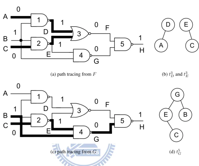
These equations and weight assignments effectively limit the total number of solutions reported by the ILP solver. However, when reconvergences of multiple faults occurs in the circuit with respect to one failing pattern, the N -net fault found by the ILP solver may no longer correctly explain the reconvergent scenario. To take Fig. 4.2 for example, based on the previous constraint, (B, E) has the weighted sum 1.75 and can be reported as one 2-net faults by the ILP solver. However, under the failing pattern, an EPO occurring on net H depends on the propagation of multiple faulty values through the nets connecting inputs of gate 3 and gate 5. opens on (B, E) fails to create a faulty value on net D connecting the input of gate 3 and thus no fault can be propagated to net F and net H will not be one EPO. To avoid generating such redundant faults, constraints called fault-propagation trees (f.p.t.) are further added for better guiding the BIP solving.
Definition: A fault-propagation tree tij is a tree for traces of signal propagataions and tra-verses backwards in the circuit topology under one failing pattern. Its root locates the net j connecting the input of a controlling-reconvergent gate i and each of its leaves lo-cates a PI or a net connecting the output of another controlling-reconvergent gate. Here a controlling-reconvergentgate denotes the gate with multiple inputs of simultaneously con-trolling values under the pattern.
Fault-propagation trees are described as individual constraints and each can be formulated into:
X
nk∈tij
nk ≤ N − 1 (4.3)
where net k is one net of the fault-propagation tree ti
j. Note that if tij consists of only one
net, the constraint is of no use and need not to be added in the BIP problem.
Each of the above constraints means that at most (N − 1) defects can occur in tij and leaves one defect in another fault-propagation tree of gate i. To take Fig. 4.2 for exam-ple again, gate 5 is one controlling-reconvergent gate and faulty values need to propagate through both net F and net G to result in an EPO on net H. Therefore, path tracing ends up with finding constraints for t5F and t5G. In Fig. 4.3(a), since gate 3 is also one controlling-reconvergent gate, the constraint for t5
F with only net F need not to be generated but two
following constraints for t3D and t3E are added accordingly. In Fig. 4.3(c), path tracing finds net B, C, E and G, for t5G in a backward manner. As result, the equations for all f.p.t. constraints are formulated as:
nA+ nD ≤ N − 1
nC + nE ≤ N − 1
nB+ nC + nE + nG ≤ N − 1
After adding these b.f.t. constraints, redundant faults such as {B, E} will not be reported by the ILP solver.
Considering the physical layout, each net in one N -net fault may consist of multiple segments and thus the size of N -segment faults can grow exponentially. For example, if a 3-net fault {A, B, C} that can be physically divided into segment set {A1, A2, A3}, {B1,
B2} and {C1, C2, C3}, respectively, the total number of 3-segment faults corresponding to
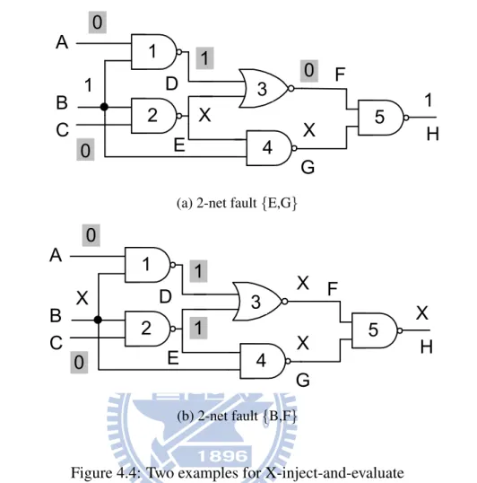
this fault is 3 × 2 × 3 = 18. To avoid the exponential growth on the size of N -segment faults, a X-inject-and-evaluate approach is first applied in step 1 and logically prune the false cases of N -net faults.
Symbolic X simulation is a common technique used in fault diagnosis and our X-inject-and-evaluate approach can be viewed as an extension of this technique. X’s are assigned on each net in one N -net fault and propagate towards the outputs simultaneously.
1
D
2
E
3
F
1
1
4
G
5
H
0
0
1
A
B
C
0
0
1
D
A
E
C
(a) path tracing from F (b) t3D and t3E
1
D
2
E
3
F
1
1
4
G
5
H
0
0
1
A
B
C
0
0
1
E
C
G
B
(c) path tracing from G (d) t5G Figure 4.3: Path tracing of fault-propagation trees
If X’s cannot be observed at all EPOs under one failing pattern, then this N -net fault is a false case and should be removed. Fig. 4.4 illustrates two examples for the X-inject-and-evaluate approach. In Fig. 4.4(a), suppose that 2-net fault (E,G) is the target. After X’s are injected on E and G, one X is blocked at gate 3 due to the controlling-value side-input connecting D. Therefore, X cannot be observed on the only EPO (net H) and thus (E,G) is removed. In Figure 4.4(b), X’s are injected on B and F and can successfully result in one X on net H. Therefore, 2-net fault (B,F ) is kept.
1
D
2
E
3
F
1
X
4
G
5
H
0
X
1
A
B
C
0
0
1
(a) 2-net fault {E,G}
1
D
2
E
3
F
1
1
4
G
5
H
X
X
X
A
B
C
0
0
X
(b) 2-net fault {B,F}Figure 4.4: Two examples for X-inject-and-evaluate
4.3
N -segment Fault Composition
During this stage, N -net faults are further verified and expanded into N -segment faults via three steps. In step 1, false net faults can be removed accordingly. Considering the lay-out of the circuit, the remaining nets of N -net faults are broken into individual segment lists that are used to compose the corresponding N -segment faults. In step 2, a physical pruning proceeds in step 1 and eliminates N -segment faults that cannot perfectly explain output responses of all patterns through fault simulation with the support of physical information. After applying X-inject-and-evaluate, step 1 starts to enumerate a list of segments for each net in the N -net faults and composes the N -segment faults from the segment lists. Before enumerating all N -segment faults from all segments of N -net faults, physical prun-ing helps to eliminate the false open segments. To further illustrate the physical prunprun-ing in
step 1, let’s use the circuit layout shown in Fig. 1.2(b) again. Suppose two faulty values appear on G3 and G4 under one failing pattern. Since an open on segment B, C or D can never result in a faulty value on G4 and an open on segment E can never result in a faulty value on G3, segment A is the only candidate on which an open can result in faulty values on G3 and G4 simultaneously. Therefore, the segment list for this net only contains {A}.
Finally, step 2 verifies if each N -segment fault can result in correct output responses under both failing and passing patterns. Such verification is done by the fault simulation with the support of physical information such as the circuit layout and the cell library. One N -segment fault will be removed if injecting opens on all segments in this fault cannot result in the matching trace of signal propagation under one either failing or passing pattern. Finally, the remaining segments in N -segment faults are treated as the true defect locations for silicon inspection.
When a segment fault are injected into the circuit, the fault on the site will take routing topology of the net, coupling capacitance, and threshold voltage of its driven gate into concern. After a pattern assigned, floating voltage is estimated by equation3.1. Then, the floating voltage is compared with the threshold voltage of driven gates to check if the fault is propagated through the driven gates. For example, as shown in Figure 1.2, assume that a fault injected on segment A. The coupling nets with logic 1 are n2, n3, and n6 while n1, n4, and n5 are logic 0. Therefore, C1 = cc2 + cc3 + cc6 and C0 = cc1 + cc4 + cc5. If the
output response mismatches, the N -segment fault will be eliminated.
4.4
Performance Comparison of Applied Constraints
During this section, the performance of applying the different constraint combinations for BIP solving is studied and Table 4.1 shows preliminary results on three small ISCAS benchmark circuits with the injection of two open defects.
The first column shows the circuit name and the second column shows the combinations of applied constraints where or, wa and fp denotes the original, weight-assignment and fault-propagation-tree constraints, respectively. The third, forth and fifth column show the total number of N -net faults that a ILP solver CPLEX generates, the total number of N -net
Table 4.1: Comparison of Applied Constraints for BIP Solving ckt const. #N nf1 #N nf2 #N sf time (s) c432 or 272.65 140.14 591.64 1.27 or+wa 139.07 77.43 424.39 0.69 or+wa+fp 92.10 62.01 310.99 0.74 c499 or 2528.41 292.59 2726.64 11.17 or+wa 487.54 256.65 2157.73 2.45 or+wa+fp 436.66 182.13 1504.51 1.94 c880 or 418.57 136.60 1353.36 2.00 or+wa 221.20 130.47 1303.53 1.62 or+wa+fp 198.90 108.94 821.64 1.53
faults after applying X-inject-and-evaluate, and the total number of N -segment faults at the end, respectively. The last column shows the runtime for N -net fault generation. As we can see, both weight-assignment and fault-propagation-tree constraints effectively reduce the total number of N -net faults as well as that of N -segment faults. Moreover, they also help reduce the runtime for N -net fault generation.
Chapter 5
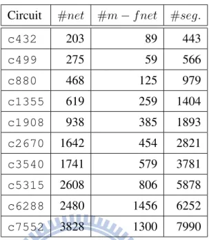
Table 5.1: Circuit Information
Circuit #net #m − f net #seg.
c432 203 89 443 c499 275 59 566 c880 468 125 979 c1355 619 259 1404 c1908 938 385 1893 c2670 1642 454 2821 c3540 1741 579 3781 c5315 2608 806 5878 c6288 2480 1456 6252 c7552 3828 1300 7990
The experiments are conducted on the ISCAS 85 benchmark circuits. The ISCAS 85 benchmark circuits, layouts and coupling capacitance information can be downloaded from TAMU website [23]. The ISCAS 85 benchmark circuits are manufactured with a 5-metal-layer TSMC 180 nm CMOS technology. Threshold voltage of each type of gate is deter-mined from SPICE simulation. To solve BIP, we use an ILP solver CPLEX. CPLEX is one of the commercial tool of LP solvers that can allow to populate all possible solutions. Each experiment includes 100 sample circuits generated with the injection of different defect sizes under 1000 patterns. Here, we inject two types of patterns to observe the influence of pattern quality.
Table 5.1 shows the gate-level and physical information of ISCAS 85 circuit. The sec-ond row shows the total number of nets. The third row shows the number of net with multiple fanouts. The forth shows the total number of segments enumerated from the cir-cuits.
5.1
Results under Random Pattern
At first, experiments on the 100 sample circuits under 1000 random patterns is ob-served. Table 5.2, 5.3, 5.4, 5.5 and 5.6 shows the result with injected random defect number N = 1, 2, 3, 4 and 5. The number of failing patterns is represented in the second row. The third row represents the number of constraints transformed from equation 4.1. The forth row represents the number of fault propagation tree constraints. The fifth row shows the number of net fault collected from net fault identification. The sixth row shows the number of N -net fault generated from N -net fault generation. The seventh row shows the number of N -segment fault composed from N -segment fault composistion.
Although hundreds of random patterns are failing patterns, there are only few con-straints generated from equation 4.1. The random patterns didn’t offer enough information of segment defects that may cause low diagnosability. Diagnosability means the ratio the number of detected fault to the number of injected fault. We will check the diagnosability of random patterns later by comparing it with the diagnosability of 5-detect patterns. During N -net fault generation, it also shows the problem that large number of fault propagation tree constraints are generated. It will cause an overhead on time if reduction of redun-dant f.p.t constraints is performed while the large number of the constraints might also cause an overhead on BIP solving time. However, compared with overhead on BIP solving time, overhead on constraint reduction time is more critical. The results shows <16 of N -segment fault are reported in average. In general, the reported number of N --segment fault is not large.
5.2
Results under 5-detect Pattern
To expect a higher diagnosability, we try to use 5-detect patterns generated from a com-mercial tool. The experiments under 1000 patterns with 5-detect patterns are conducted. Table 5.7 shows the number of 5-detect patterns generated from the commercial tool. Ta-ble 5.8, 5.9, 5.10, 5.11, and 5.12 shows the experimental result with injected random defect number = 1, 2, 3, 4, and 5 with 5-detect patterns.
T able 5.2: N =1 under 1000 random patterns ckt # f pttn # eq (4) const # f pt const # nf # N nf # N sf C P U time c432 314.3 23.1 695107.5 137.7 13.5 2.2 0.7 c499 151.5 6.7 41609.8 140.0 49.2 2.9 2.1 c880 325.0 11.3 184720.8 97.6 17.4 2.1 1.5 c1355 218.2 8.7 62897.9 334.8 96.9 8.3 2.5 c1908 285.0 13.4 91843.9 522.4 61.6 4.3 6.9 c2670 247.8 9.7 253430.2 174.6 57.8 3.4 5.8 c3540 161.8 14.9 1122794.0 729.5 78.8 3.0 13.8 c5315 163.0 9.2 122795.9 211.5 62.4 4.0 20.2 c6288 236.2 14.7 1054766.8 1269.4 573.7 1.8 45.3 c7552 204.6 11.9 312881.7 398.3 84.4 2.4 13.2 a vg 230.7 12.4 394284.8 405.9 109.6 3.4 11.2
T able 5.3: N =2 under 1000 random patterns ckt # f pttn # eq (4) const # f pt const # nf # N nf # N sf C P U time c432 323.7 25.9 15025.2 137.8 186.7 2.6 2.9 c499 218.4 10.4 74704.2 151.2 307.2 3.6 12.6 c880 394.6 14.8 233257.8 128.6 133.4 3.2 3.8 c1355 436.8 8.6 33911.2 288.8 476.1 7.7 53.5 c1908 385.8 10.2 75374.6 538.5 1431.2 6.4 263.9 c2670 255.1 6.5 23609.8 227.6 181.5 4.5 57.5 c3540 205.8 12.1 103454.8 726.6 301.1 3.0 68.2 c5315 115.7 35.1 88578.8 387.9 768.6 2.2 158.2 c6288 270.5 33.3 949998.1 1743.7 1850.3 1.4 350.4 c7552 440.2 9.4 48506.1 586.3 1497.7 8.2 238.2 a vg 304.7 16.4 791420.5 491.7 713.4 4.3 89.4
T able 5.4: N =3 under 1000 random patterns ckt # f pttn # eq (4) const # f pt const # nf # N nf # N sf C P U time c432 408.1 27.9 16187.8 148.6 89.8 2.2 2.8 c499 381.4 16.1 3137.6 140.7 81.6 3.3 28.7 c880 698.2 35.2 13337.3 202.3 155.8 7.0 24.2 c1355 308.3 13.1 2021.4 391.4 1014.8 5.2 159.5 c1908 381.3 15.2 14505.7 516.3 260.4 1.3 362.9 c2670 254.3 5.5 6839.5 284.8 779.9 1.5 369.7 c3540 199.5 13.2 18544.3 895.8 818.3 2.0 408.7 c5315 324.7 42.7 6921.6 310.8 4363.3 8.5 723.4 c6288 187.0 30.1 63512.0 1153.1 1178.5 1.6 1232.0 c7552 259.6 10.1 7843.2 421.0 8430.3 5.5 743.6 a vg 340.3 20.9 15285.0 446.5 1717.3 3.8 405.5
T able 5.5: N =4 under 1000 random patterns ckt # f pttn # eq (4) const # f pt const # nf # N nf # N sf C P U time c432 414.4 360.5 29856.5 195.1 37386.5 3.6 253.9 c499 372.4 255.1 5282.3 172.2 41977.6 5.7 572.2 c880 634.3 448.3 4062.0 189.2 4852.4 4.2 443.4 c1355 322.1 96.3 3194.7 429.9 4293.2 4.7 588.0 c1908 390.0 24.1 30151.1 533.4 11360.0 3.2 1523.9 c2670 281.3 117.7 7218.3 305.3 2139.5 4.1 977.2 c3540 124.0 24.7 16383.6 1051.7 13303.4 3.0 1055.5 c5315 391.7 159.4 5120.3 492.5 37237.8 6.0 2271.4 c6288 403.5 26.1 43103.5 1612.4 56130.3 2.8 4769.3 c7552 312.3 89.1 11357.0 566.3 30246.9 5.5 2691.6 a vg 364.6 160.1 11573.0 464.8 23892.7 4.3 1514.6
T able 5.6: N =5 under 1000 random patterns ckt # f pttn # eq (4) const # f pt const # nf # N nf # N sf C P U time c432 422.1 388.2 17327.6 188.3 2303.0 5.3 523.4 c499 382.7 213.6 6248.6 192.4 51296.6 13.7 1135.3 c880 658.3 401.1 8732.0 200.7 7892.3 6.2 622.2 c1355 331.6 133.6 2937.4 473.0 3376.4 6.5 733.6 c1908 362.5 37.5 22171.2 557.4 112374.1 10.3 11790.0 c2670 240.1 155.3 6293.8 352.2 8237.5 7.4 1531.6 c3540 239.2 52.3 10936.1 1167.9 32562.2 6.0 1922.1 c5315 417.2 157.0 4092.3 479.0 76237.2 7.3 3901.3 c6288 385.5 23.2 24967.8 1663.6 213968.3 15.3 15609.9 c7552 339.0 105.2 3825.6 592.2 137274.7 6.3 8832.6 a vg 377.8 166.7 10753.2 586.7 64552.2 8.4 3860.2
Table 5.7: 5-Detect Stuck-at Pattern Circuit #5 − dpttn. Circuit #5 − dpttn. c432 225 c2670 286 c499 267 c3540 528 c880 182 c5315 297 c1355 432 c6288 81 c1908 591 c7552 460
offers more information of open defects than under random patterns. The results also shows that the number of N -segment faults are < 9 which is less than the results under random patterns. In most cases, the reported N -segment faults under 5-detect patterns are also less than under random patterns.
5.3
Diagnosability and Resolution Comparison
Results comparison between 5-detect pattern and random pattern of four circuits are being discussed. Resolusion means the ratio the number of fault reported to the number of fault detected. Here, we define net resolusion and segment resolusion to discriminate the results of reported net and reported segment, respectively. Figure 5.1 and Figure 5.2 shows the comparison of net resolusion and segment resolusion. Resolution under random patterns is generally higher than under 5-detect patterns. The results shows that we don’t need the inspect many signal lines to find the open segment defects. The approach gives an accurate result to find segment defects.
Figure 5.3 shows the diagnosability comparison. Diagnosability under random patterns decreases quickly when open defect size N increases. With less constraints, random pat-terns offers less information of open defects. Therefore, pattern quality determines the diagnosability. The reason that the decreasing of diagnosability results from the activation and propagation of open segment faults. If the given patterns fails to expose the charac-teristics of all faults, only the subset of faults can be identified with limited information.
T able 5.8: N =1 under 5-detect stuck-at patterns ckt # f pttn # eq (4) const # f pt const # nf # N nf # N sf C P U time c432 104.4 177.5 5030.2 170.0 11.0 1.7 0.27 c499 206.4 137.1 615.4 196.5 49.5 1.8 0.41 c880 252.0 129.8 2619.3 143.8 12.8 1.6 0.19 c1355 494.5 431.9 1922.1 508.0 33.3 1.5 2.77 c1908 555.2 844.0 27135.3 679.7 42.0 1.4 9.72 c2670 121.6 112.6 2678.1 538.2 50.4 2.6 1.07 c3540 187.8 299.3 23871.9 1245.1 27.4 1.7 7.52 c5315 149.2 217.1 3003.3 631.9 27.8 1.4 1.75 c6288 186.3 83.0 16566.0 1629.1 355.8 1.4 23.34 c7552 347.0 473.7 10632.4 869.1 42.4 1.4 7.06 a vg 260.4 290.6 9407.4 661.1 65.2 1.6 5.41
T able 5.9: N =2 under 5-detect stuck-at patterns ckt # f pttn # eq (4) const # f pt const # nf # N nf # N sf C P U time c432 187.0 343.5 10751.0 180.4 186.5 2.4 7.0 c499 263.4 174.9 877.5 196.7 1817.4 2.3 70.2 c880 336.1 181.9 4391.5 167.6 98.9 2.1 3.8 c1355 742.0 672.8 3302.2 532.7 2817.5 1.9 212.4 c1908 864.0 1345.2 49030.6 767.9 3678.7 3.0 113.4 c2670 212.2 193.4 4911.4 707.8 1374.6 3.3 399.5 c3540 349.3 530.2 40906.3 1388.6 1309.4 1.7 370.0 c5315 227.1 265.9 3532.9 791.9 1093.6 1.8 178.1 c6288 71.6 52.3 7080.9 2216.6 428.2 1.3 1754.2 c7552 723.1 534.9 15016.3 732.5 8243.4 5.5 1753.6 a vg 397.6 429.5 13980.0 768.3 2104.8 2.5 486.2
T able 5.10: N =3 under 5-detect stuck-at patterns ckt # f pttn # eq (4) const # f pt const # nf # N nf # N sf C P U time c432 396.5 847.5 26064.0 195.0 5237.2 4.5 97.7 c499 398.7 336.1 2188.0 199.1 37501.7 3.3 182.8 c880 457.9 271.9 6887.6 219.6 1303.3 3.0 157.2 c1355 792.8 589.7 5698.9 570.8 9132.4 5.5 1052.7 c1908 235.5 313.5 11383.3 706.7 1770.4 2.9 477.2 c2670 253.5 196.4 6839.6 1096.4 799.5 2.6 377.0 c3540 97.5 56.4 7994.2 1399.3 54.2 1.6 819.9 c5315 342.7 649.7 6921.0 1080.1 5131.5 2.2 1074.3 c6288 133.8 32.6 14618.4 1687.9 1707.4 1.4 1302.4 c7552 259.6 109.2 3921.6 420.1 5226.1 5.4 1140.2 a vg 336.8 340.3 9251.7 757.5 6786.3 3.2 694.8
T able 5.11: N =4 under 5-detect stuck-at patterns ckt # f pttn # eq (4) const # f pt const # nf # N nf # N sf C P U time c432 413.3 249.1 16230.4 201.6 3910.0 2.1 202.7 c499 421.5 383.6 5135.5 221.7 13060.6 2.8 561.1 c880 523.5 632.1 23413.1 306.4 11342.8 7.3 875.1 c1355 801.1 611.7 9922.0 562.5 10982.3 5.2 2031.8 c1908 351.4 492.3 6732.9 746.1 6089.1 3.2 1131.4 c2670 302.9 518.2 7671.7 1503.0 5266.2 4.0 953.3 c3540 114.7 203.1 62329.5 1529.3 4865.1 6.2 1722.6 c5315 486.2 492.0 18721.3 1277.1 6844.5 6.6 2218.0 c6288 522.1 63.7 187831.6 1913.2 29131.3 5.9 3862.9 c7552 430.1 183.5 37288.2 593.2 37079.4 8.5 2993.1 a vg 436.7 382.9 37527.6 885.4 12857.1 5.2 1655.2
T able 5.12: N =5 under 5-detect stuck-at patterns ckt # f pttn # eq (4) const # f pt const # nf # N nf # N sf C P U time c432 462.3 230.1 9235.3 187.1 1205.5 3.2 852.3 c499 452.2 329.3 6266.3 237.1 7264.1 3.7 1336.6 c880 544.3 583.2 22398.5 293.5 8883.2 4.4 927.3 c1355 793.2 620.2 10344.8 525.3 13532.6 5.2 4592.8 c1908 334.5 408.8 7295.5 662.6 3021.0 5.8 17032.6 c2670 329.0 493.3 7327.6 1341.3 1793.2 3.1 4319.3 c3540 122.2 221.6 43106.0 1472.4 2395.1 4.6 5192.2 c5315 493.2 526.4 13681.1 1362.3 5927.0 6.6 5036.3 c6288 502.3 48.0 73266.4 1966.3 39138.2 8.1 23152.5 c7552 428.9 200.3 36207.3 475.6 23962.2 6.9 20207.4 a vg 436.7 366.1 22912.8 848.6 10712.2 5.2 8264.9
0 1 2 3 4 1 2 3 4 5 N e t R e s o lu tio n Defect Number c3540 random 5-detect 0 1 2 3 4 1 2 3 4 5 N e t R e s o lu tio n Defect Number c5315 random 5-detect (a) (b) 0 1 2 3 4 1 2 3 4 5 N e t R e s o lu tio n Defect Number c6288 random 5-detect 0 1 2 3 4 1 2 3 4 5 N e t R e s o lu tio n Defect Number c7552 random 5-detect (c) (d)
Figure 5.1: Net resolution
For example, as shown in Figure 5.4, suppose that four open-segment defects are injected. Segment f 1 solely explain EPOs for pattern p1 and f 1, f 2 and f 4 jointly explain EPOs for p2. f 2 solely explains p3 and p4, and f 3 cannot explain any patterns. Because the defect on segment f 3 and f 4 cannot be observed through the entire simulation, only f 1 and f 2 are detectable. Therefore, if the given patterns can provide more constraints, the proposed approach can report the N -segment fault more precisely.
An open segment fault may not be obsered from fault masking and fault covering Fault masking means the fault is masked during propagation as shown in Figure 5.5(a). The fault cannot be oberseved from outputs in this case. Fault covering means the faults propagate to
0 1 2 3 4 1 2 3 4 5 S e g m e n t R e s o lu tio n Defect Number c3540 random 5-detect 0 1 2 3 4 1 2 3 4 5 S e g m e n t R e s o lu tio n Defect Number c5315 random 5-detect (a) (b) 0 1 2 3 4 1 2 3 4 5 S e g m e n t R e s o lu tio n Defect Number c6288 random 5-detect 0 1 2 3 4 1 2 3 4 5 S e g m e n t R e s o lu tio n Defect Number c7552 random 5-detect (a) (b)
Figure 5.2: Segment resolution
EPOs through the same subpaths as shown in Figure 5.5(b). Assuming that a fault FAcan
cause EPOs EOA, and fault FBcan cause EPOs EOB. If EOA⊂EOB, FBis prompt to be
considered as the real fault but not FA. Although FA is covered by FB, we can diagnose
FB. Fault masking often results from logic masking during fault propagation for multiple
stuck-at faults. For multiple open segment faults, fault masking may also results from fault activation. An open segment fault can inactivate another fault by affecting logic value of its coupling nets. This case represents more complex fault correlation for open segment fault. However, as long as the open segment faults can be traced from net fault generation, our approach can generate N -net faults correspondingly explain the output response.
0 20 40 60 80 100 1 2 3 4 5 D ia g n o s a b il it y ( % ) Defect Number c3540 5-detect random 0 20 40 60 80 100 1 2 3 4 5 D ia g n o s a b il it y ( % ) Defect Number c5315 5-detect random (a) (b) 0 20 40 60 80 100 1 2 3 4 5 D ia g n o s a b il it y ( % ) Defect Number c6288 5-detect random 0 20 40 60 80 100 1 2 3 4 5 D ia g n o s a b ilit y ( % ) Defect Number c7552 5-detect random (c) (d) Figure 5.3: Diagnosability
Pattern
p1
p2
p3
p4
f1
f2
f3
f4
Never activated
Figure 5.4: Fault Detection According to Simulation Result
F
AF
BF
BF
A(a) fault masking (b) fault covering
Chapter 6
Conclusion
The Byzantine effect makes faulty behavior due to an open segment nondeterminis-tic and thus diagnosing multiple open-segment defects is more difficult than diagnosing a single one. Fault activation and propagation depends on both patterns and the physical in-formation. In this paper, a three-stage diagnosis approach is proposed to generate rational N -segment fault as faults and consists of net fault identification, N -net fault generation and N -segment fault composition. We also discussed the technique we use to reduce the number of N -net fault generated from ILP solver. For each ISCAS85 circuits, experiments are conducted on 100 different samples with the random injection of 1 to 5 open segments under random patterns and 5-detect patterns. Final results show that the proposed approach can effectively generate a small number (<16) of N -segment fault under random patterns and a smaller number (<9) under 5-detect patterns for all ISCAS85 benchmark circuits. Results under 5-detect patterns also has higher diagnosability than under random patterns. It shows that higher pattern quality generates higher diagnosability. Therefore, diagnostic pattern generation for open segment fault helps to deal with the patter quality issue.
Bibliography
[1] S. Y. Huang, ”Diagnosis of Byzantine Open-Segment Faults”, Proc. Asian Test Symp. (ATS), pp. 248-253, Nov. 2002.
[2] W. Zou, W. T. Cheng and S. M. Reddy, ”Interconnect open defect diagnosis with phys-ical information”, Proc. Asian Test Symp. (ATS), pp. 203-209, Nov. 2006.
[3] X. Yu and R. D. Blanton, ”Multiple defect diagnosis using no assumption on fail-ing pattern characteristics”, Proc. Design Automation Conf. (DAC), pp. 361-366, Jun. 2008.
[4] W. C. Tam, O. Poku and R. D. Blanton, ”Automated failure population creation for val-idating integrated circuit diagnosis methods”, Proc. Design Automation Conf. (DAC), pp. 708-713, Jul. 2009.
[5] Y. C. Lin and K. T. Cheng, ”Multiple-fault diagnosis based on single-fault activation and single-output observation”, Proc. Design, Automation and Test in Europe Conf. (DATE), pp. 1-6, Mar. 2006.
[6] C. F. Hawkins, J. M. Soden, A. W. Righter and F. J. Ferguson, ”Defect classes - An overdue paradigm for CMOS IC testing”, Proc. Int’l Test Conf. (ITC), pp. 413-425, Oct. 1994.
[7] T. Bartenstein, D. Heaberlin, L. Huisman and D. Sliwinski, ”Diagnosing combinational logic designs using single location at-a-time (SLAT) paradigm”, Proc. Int’l Test Conf. (ITC), pp. 287-296, Oct. 2001.
[8] J. B. Liu, A. Veneris and H. Takahashi, ”Incremental diagnosis of multiple open-interconnects”, Proc. Int’l Test Conf. (ITC), pp. 1085-1092, Oct. 2002.
[9] Y. Sato, I. Yamazaki, H. Yamanaka, T. Ikeda and M. Takakura, ”A persistent diagnostic technique for unstable defects”, Proc. Int’l Test Conf. (ITC), pp. 242-249, Oct. 2002.
[10] X. Lin and J. Rajski, ”Test generation for interconnect opens”, Proc. Int’l Testing Conf. (ITC), pp. 1-7, Oct. 2008.
[11] J. B. Liu, A. Veneris and M. S. Abadir, ”Efficient and exact diagnosis of multiple stuck-at faults”, Proc. Latin-American Test Workshop (LATW), Feb. 2002.
[12] S. Venkataraman and S. B. Drummonds, ”A technique for logic fault diagnosis of interconnect open defects”, Proc. VLSI Test Symp. (VTS), pp. 313-318, Apr. 2000.
[13] X. Fan, W. Moore, C. Hora, M. Konijnenburg and G. Gronthoud, ”A gate-level method for transistor-level bridging fault diagnosis”, Proc. VLSI Test Symp. (VTS), pp. 266-271, Apr. 2006.
[14] S. Spinner, I. Polian, P. Engelke, B. Becker, ”Automatic test pattern generation for interconnect open defects”, Proc. of VLSI Test Symp. (VTS), pp. 181-186, Apr. 2008.
[15] Z. Wang, M. M. Sadowska, K. H. Tsai and J. Rajski, ”Multiple fault diagnosis using n-defection tests”, Proc. Int’l Conf. Computer Design (ICCD), pp. 198-201, Oct. 2003.
[16] H. Sue, C. Di and J. A. G. Jess, ”Probability analysis for CMOS floating gate faults,” Proc. Europe Design Test Conf. (EDTC), pp. 443-448, Feb. 1994.
[17] C. Y. Kao, C. H. Liao, and H. P. Wen, ”An ILP-based diagnosis framework for multiple open defects”, Proc. Int’l Microprocessor Testing and Verification Workshop (MTV), pp. 69-72 Dec. 2009.
[18] X. Wen, H. Tamamoto, K. K. Saluja and K. Kinoshita, ”Fault diagnosis for physical defects of unknown behaviors”, IEEE Asian Test Symp. (ATS), pp. 236-241, Nov. 2003.
[19] Y. C. Lin, F. Lu, and K. T. Cheng, ”Multiple-fault diagnosis based on adaptive di-agnostic test pattern generation”, IEEE Tran. CAD of Integrated Circuits and Systems (TCAD), vol. 26, pp. 932-942, May 2007.
[20] S. Y. Huang, ”A symbolic inject-and-evaluate paradigm for byzantine fault diagno-sis”, Jour. Electronic Testing: Theory and Application (JETTA), vol. 19, pp. 161-172, Oct. 2003.
[21] Y. Takamatsu,T. Seiyama, H. Takahashi,Y. Higami, and K. Yamazaki, ”On the fault diagnosis in the presence of unknown fault models using pass/fail information”, Int’l Symp. Circuits and Systems (ISCAS) pp. 2987-2990, Vol. 3, May. 2005.
[22] M. Renovell and G. Cambon, ”Electrical analysis and modeling of floating-gate fault”, IEEE Tran. CAD of Integrated Circuits and Systems (TCAD), pp. 1450-1458, vol. 11, Nov. 1992.
[23] The TAMU Website, http://dropzone.tamu.edu/ xiang/iscas.html
[24] R. Rodriguez-Montanes, D. Arumi, S. Einchenberger, C. Hora, B. Kruseman and M. Lousberg, ”Diagnosis of Full Open Defects in Interconeecting Lines”, Proc. VLSI Test Symp. (VTS), pp. 158-166, May. 2007.
[25] Z. Wang, M. Marek-Sadowska, K.-H. Tsai and J. Rajski, ”Analysis and Methodology for Multiple-Fault Diagnosis”, IEEE Tran. CAD of Integrated Circuits and Systems (TCAD), pp. 559-575, vol.25, Mar. 2006.
[26] S. Hillebrecht, I. Polian, P. Engelke, B. Becker, M. Keim and W.-T. Cheng, ”Ex-traction, Simulation adn Test Generation for Interconnect Open Defects Based on En-hanced Aggressor-Victim Model”, Proc. Int’l Testing Conf. (ITC), pp. 1-10, Oct. 2008.
[27] S. M. Reddy, I. Pomeranz, H. Tang, S. Kajihara and K. Kinoshita, ”On Testing of Interconnect Open Defects in Combinational Logic Circuits with Stems of Large Fanout”, Proc. Int’l Testing Conf. (ITC), pp. 83-89, Oct. 2002.