上鏈LTE單載波頻分多址技術之研究

國 立 交 通 大 學

電信工程研究所

碩 士 論 文

上鏈 LTE 單載波頻分多址技術之研究

A Study of Single-Carrier Frequency-Division Multiple

Access in Long-term Evolution Uplink

研 究 生：余日翔

指導教授：黃家齊 博士

上鏈 LTE 單載波頻分多址技術之研究

A Study of Single-Carrier Frequency-Division Multiple Access in

Long-term Evolution Uplink

研 究 生：余日翔 Student：Rih-Hsiang Yu

指導教授：黃家齊 博士 Advisor：Dr. Chia-Chi Huang

國 立 交 通 大 學

電信工程研究所

碩 士 論 文

A Thesis

Submitted to Institute of Communication Engineering College of Electrical and Computer Engineering

National Chiao Tung University in partial Fulfillment of the Requirements

for the Degree of Master in

Communication Engineering November 2013

Hsinchu, Taiwan, Republic of China

i

上鏈 LTE 單載波頻分多址技術之研究

研究生: 余日翔 指導教授: 黃家齊博士

國立交通大學電信工程研究所 碩士班

摘 要

現行第三代合作夥伴計劃(3GPP)長期演進技術(LTE)中，使用正交頻分多址 (OFDMA)於下行鏈路以及使用單載波頻分多址(SC-FDMA)於上行鏈路。單載波頻分多 址是正交頻分多址的一種改進形式，它是一種在高數據速率傳輸下很有效率的技術。在 我們的研究中，我們分析了長期演進技術上行鏈路的數據調變、子載波分配的方法、降 低峰均功率比(PAPR)的技術和系統層面的資源塊(resource block)分配。我們觀察到，在 集中式單載波頻分多址(Localized SC-FDMA, LFDMA)的峰均功率比性能比正交頻分多 址稍微好一點，但遠不如交錯的分布式單載波頻分多址(Interleaved SC-FDMA, IFDMA)， 所以我們設計了一個反饋搜索選擇性映射擾碼(Feedback-searching selective mapping)和 符號替代方法(Symbol-replaced method)來降低集中式單載波頻分多址的峰均功率比。模 擬結果比較了這兩種方法和基本的選擇性映射擾碼再降低峰均功率比上的表現。最後， 我們提出了一個誤碼率增強貪婪式演算法(BER-enhanced greedy method)，在某些假設條 件下資源塊可以被分配更有效率。模擬結果表示，此方法誤碼率(BER)的性能有很好的 提升。

ii

A Study of Single-Carrier Frequency Division Multiple Access in

Long-term Evolution Uplink

Student: Jih-Hsiang Yu Advisor: Dr. Chia-Chi Huang

Institute of Communication Engineering

National Chiao Tung University

ABSTRACT

The current standard in 3rd Generation partnership project (3GPP) Long-Term Evolution (LTE) uses orthogonal FDMA (OFDMA) for downlink and single carrier FDMA (SC-FDMA) for uplink. SC-FDMA is a modified form of OFDMA, and it is a promising technique for high data rate transmission. In our research, we analyze the LTE uplink in the data modulations, subcarrier mapping schemes, techniques for PAPR reduction and resource allocations. We observe that the PAPR performance in localized SC-FDMA (LFDMA) is slightly better than OFDMA, but much worse than interleaved SC-FDMA (IFDMA), so we design feedback searching selective mapping and symbol-replaced methods that reduce the PAPR of LFDMA signals. The numerical results reveal their performance in reducing PAPR compared with basic SLM. Finally we propose a BER-enhanced greedy method, which assigns the resource blocks more efficiently under certain assumptions. The simulation results show that the proposed method has a great performance improvement in bit error rate (BER).

iii

誌 謝

首先感謝黃家齊老師這兩年來，對於我的研究、課業與生活上的指導與勉勵，以及 對於論文內容的建議，使我得以完成碩士學位。同時感謝口試委員陳紹基教授與余誌民 教授給予的寶貴意見與指教，使得本論文更加完整。 特別感謝馬峻楹與蕭煒翰學長在我研究過程中給予的巨大幫助，讓我的觀念更加清 楚、紮實。感謝我實驗時的同學冠銘、健瑋以及雅涵以及學弟妹的砥礪與照顧，並帶給 實驗室很多的歡樂。 謝我的家人給予我的關心與經濟上的支持，你們是我最大的支柱，讓我能無後顧之 憂地完成學業，最後再次感謝所有人，讓我有個非常精彩的碩士生活。

iv

TABLE OF CONTENTS

中文摘要 i ABSTRACT ii 誌謝 iii LIST OF FIGURES vi

LIST OF TABLES viii

CHAPTER 1 INTRODUCTION 1

CHAPTER 2 BASIC CONCEPT IN SC-FDMA FOR LTE UPLINK

2.1 Overview of the SC-FDMA Structure ……… 2.2 Data Modulations………. 2.3 Subcarrier Mapping………. 2.4 Cyclic Prefix Insertion………. 2.5 Characteristic of Wireless Mobile Communication Channel………….. 2.6 Simulation……… 2.6.1 Simulation parameters……….. 2.6.2 Simulation block diagram………. 2.6.3 Simulation channel model……… 2.6.4 Simulation added noise at receiver………... 2.6.5 Simulation MMSE frequency domain equalization………. 2.6.6 Simulation result………... 2.7 Conclusion of Chapter 2……….. 3 3 6 10 11 12 14 14 14 15 16 17 17 20

CHAPTER 3 PAPR REDUCTION FOR LOCALIZED SC-FDMA

3.1 Time domain symbol analysis of SC-FDMA……….. 3.1.1 Time domain symbols of IFDMA……… 3.1.2 Time domain symbols of LFDMA……… 3.1.3 Comparison of 99.9-percentile PAPR……….. 3.2 Basic SLM for PAPR Reduction………. 3.2.1 Block diagram of basic SLM……… 3.2.2 Formulation of Basic SLM transmitter………. 3.2.3 Side Information………... 3.3 Proposed Feedback-searching SLM for PAPR Reduction……….. 3.3.1 Block diagram of the proposed feedback-searching SLM………… 3.3.2 Algorithm for the proposed feedback-searching SLM………. 3.3.3 Comparison of computation complexity with basic SLM………… 3.4 Symbol-replaced Methods for PAPR Reduction……….

22 22 22 25 27 28 28 29 30 31 31 31 32 32

v

3.4.1 Block diagram of the symbol-replaced method……… 3.4.2 Algorithm for the symbol-replaced method………. 3.4.3 Improved Feedback-searching symbol-replaced method…………. 3.5 Simulation ……….. 3.5.1 Simulation parameters….……… 3.5.1 Simulation results………. 3.6 Conclusion of Chapter 3……….. 32 33 34 35 35 36 39

CHAPTER 4 RECOURCE ALLOCATION IN LTE UPLINK

4.1 System Model and Transmission Schemes………. 4.2 Problem Formulation………... 4.3 Greedy Method……… 4.4 Maximum Greedy Method……….. 4.5 Proposed BER-Enhanced Greedy Method……….. 4.6 Comparison of Computation among these three methods………... 4.7 Simulation……… 4.7.1 Simulation parameters……….………. 4.7.2 Simulation results………. 4.8 Conclusion of Chapter 4……….. 40 40 41 42 43 44 45 46 46 46 47 REFERENCES 48

vi

LIST OF FIGURES

Figure page

2.1 Transmitter and receiver structure of the SC-FDMA system 3 2.2 Transmitter and receiver structure of the OFDMA system 3

2.3 Raised-cosine filter 5

2.4 Generation of SC-FDMA transmitter symbols 6

2.5 BPSK mapping 7

2.6 QPSK mapping 7

2.7 16-QAM and 64-QAM mapping 8 2.8 Time domain symbols transform to frequency domain by applying FFT 9 2.9 Subcarrier mapping mode 10 2.10 Subcarrier allocation methods for multiple users (3 users, 12 subcarriers,

and 4 subcarriers allocated per user)

11 2.11 Cyclic prefix insertion 11 2.12 Frequency response of PedA. channel and 6-tap typical urban (TU6)

channel over 512 subcarriers.

13 2.13 Block diagram of SC-FDMA simulator 14 2.14 BER performance of LFDMA for ideal channe 17 2.15 BER performance of IFDMA for ideal channel 18 2.16 BER performance of LFDMA for PedA. channel 18 2.17 BER performance ofIFDMA for PedA. channel 19 2.18 BER performance of LFDMA for TU6 channel 19 2.19 BER performance of IFDMA for TU6 channel 20 3.1 Illustration of IFDMA subcarrier mapping for N=4, Q=3 M=12 23 3.2 Illustration of LFDMA subcarrier mapping for N=4, Q=3 M=12 25 3.3 An example of IFDMA transmitting signals (M=16, N=4) 26 3.4 An example of LFDMA transmitting signals (M=16, N=4) 26 3.5 Time domain symbols of IFDMA and LFDMA 27 3.6 Block diagram of basic SLM for SC-FDMA system-transmitter 28 3.7 Block diagram of basic SLM for SC-FDMA system-receiver 28 3.8 An example of C position combination that N=5, K=2 30

vii

3.9 Block diagram of the proposed SLM for SC-FDMA system-transmitter 31 3.10 Block diagram of symbol-replaced method for SC-FDMA

system-transmitter

32 3.11 An example of the symbol-replaced method. (B=5) 33 3.12 Block diagram of Feedback-searching symbol-replaced method for

SC-FDMA system-transmitter

34 3.13 The BER performance of two different symbol-replaced methods 36 3.14 The BER performance of three different methods under similar complexity. 36 3.15 BER performance of basic SLM over different C values. 37 3.16 The BER performance of FS-SLM over different C values. 37 3.17 The BER performance of different PAPR reduction methods over different

SNR values in ideal channel.

38 3.18 The BER performance of different PAPR reduction methods over different

SNR values in PedA. channel.

38 4.1 Block diagram of the whole SC-FDMA system 40 4.2 The subcarrier occupations between different users. 40 4.3 A simple example of greedy method 42 4.4 A simple example of maximum greedy method 43 4.5 A simple example of BER-enhanced greedy method 44 4.6 The effect on BER performance for different SNR 44 4.7 The effect on BER performance for different number of users 47

viii

LIST OF TABLES

Table page

2.1 Power delay profiles of PedA. channel and TU6 channel. 13 2.2 Simulation parameters of Chapter 2. 14 3.1 Comparison of 99.9-percentile PAPR 27 3.2 Comparison of computation complexity with two SLMs 32 3.3 Simulation parameters of Chapter 3. 35 4.1 Comparison of computation complexity among these three methods. 45 4.2 Simulation parameters of Chapter 4. 46

1

CHAPTER 1

INTRODUCTION

The cellular technologies specified by 3rd Generation Partnership Project (3GPP) are widely deployed in the world. 3GPP Long Term Evolution (LTE) holds a project to improve the mobile phone standard to cope with future requirement. In this thesis, we investigate the uplink technologies of 3GPP LTE, which is a transmission technique that utilize the Single-Carrier Frequency-Division Multiple Access (SC-FDMA), a modified form of orthogonal FDMA (OFDMA). SC-FDMA is a promising technique for high data rate uplink communications in cellular systems. It has similar throughput performance and essentially the same overall complexity as OFDMA. The principal advantages of SC-FDMA are that it utilizes frequency domain equalizations and its transmitter structure leads to a low PAPR (Peak-to-average Power Ratio), which is related to the energy consumptions.

First in this thesis, we analyze the LTE uplink in the basic structures, which contain the data modulations, subcarrier mappings, and cyclic prefix (CP) insertion, and compare the bit error rate in different data modulations and different subcarrier mapping schemes over different channels. Furthermore, we analyze the time domain signals of two subcarrier mapping schemes and find that PAPR in localized SC-FDMA (LFDMA) is not as good as interleaved SC-FDMA (IFDMA). So we investigate the techniques for PAPR reduction and propose a feedback searching selective mapping and symbol-replaced method. Finally, we investigate the uplink LTE resource allocations under certain assumptions and propose a BER-enhanced greedy method to assign the resource blocks to the users with bad channel gains in high priorities to enhance the BER performance for the whole system

2

The rest of this thesis is organized as follows. In Chapter 2, we analyze the BER performance over different data modulations, subcarrier mapping schemes and three multipath fading channel. In Chapter 3, we start with the time domain symbols of LFDMA and IFDMA, and it shows that the PAPR performance of LFDMA is not as good as IFDMA. So we analyze a common method used in reducing PAPR, selective mapping (SLM). Then we propose a feedback searching SLM and symbol-replaced methods to reduce the PAPR for LFDMA. In Chapter 4, assuming that all users can be allocated by only one resource block, we investigate 3 common algorithms, direct approach, greedy method and maximum greedy method. Then we design a BER-enhanced greedy method to assign the resource block prior to the user with lowest total channel gain. Finally, each chapters give their own conclusions because it is not so related to each other. It should be noted that chapter 2, 3 and 4 have their own system models.

Throughout this thesis, we adopt some notations: Matrix and vectors are denoted by uppercase and lower case boldface letters; 𝐈_𝑁 is the 𝑁 × 𝑁 identity matrix; 𝐅_𝑀 is the M-point FFT transform matrix. A [i,j] indicates the element in the row i and column j of the matrix A. (∙)∗, (∙)𝑇 and (∙)𝐻 represent the conjugate, transpose and Hermitian transpose operators. ⊗ represents the point-wised multiplication of two vectors.

3

CHAPTER 2

Basic Concept in SC-FDMA for LTE Uplink

Figure 2.1: Transmitter and receiver structure of the SC-FDMA system.

Figure 2.2: Transmitter and receiver structure of the OFDMA system.

2.1 Overview of the SC-FDMA Structure

Figure 2.1 shows a block diagram of a SC-FDMA system. SC-FDMA can be regard as DFT-spread OFDMA, where time domain data symbols are transformed into frequency domain by DFT (Discrete Fourier Transform) before going through OFDMA modulation. The

4

orthogonality of users stems from the fact that different users occupies different subcarriers in the frequency domain, similar to the case of OFDMA. Because the overall transmit signal is a single carrier signal, PAPR inherently low compared to the case of OFDMA which produces a multicarrier signal.

At the input to the transmitter, a baseband modulator transforms the binary input to a multilevel sequence of complex numbers x in one of several possible modulation formats. The transmitter next groups the modulated symbols {x} into blocks each containing N symbols. The first step in modulating the SC-FDMA subcarrier is to perform an N-point FFT to produce a frequency domain representation {X} of the input symbols. Then it maps N FFT outputs to one of the M (>N) orthogonal subcarriers that will be transmitted. If N = M/Q and all terminals transmit N symbols per block, the system can handle Q simultaneous transmission without co-channel interference. Q is the bandwidth expansion factor of the SC-FDMA system. The result of the subcarrier mapping is the set {𝑋̃} with N non-zero complex amplitudes. As in OFDMA, an M-point IFFT transforms the subcarrier amplitudes to a complex time domain signal {𝑥̃}.

The transmitter perform two other signal processing prior to transmission. It insert a set of symbols referred to as a cyclic prefix in order to provide a guard time interval to prevent inter-symbol interference (ISI) caused by multipath propagation. The transmitter also performs a linear filtering operation referred to as pulse shaping in order to reduce the out-of-band signal energy.

Cyclic prefix (CP) is a copy of the last part of the block. It acts as a guard time interval between successive blocks, and since CP is a copy of the last part of the block, it converts a discrete time linear convolution into a discrete time circular convolution. Thus the received symbol can be modeled as a circular convolution between the channel impulse response and transmitted data block.

5

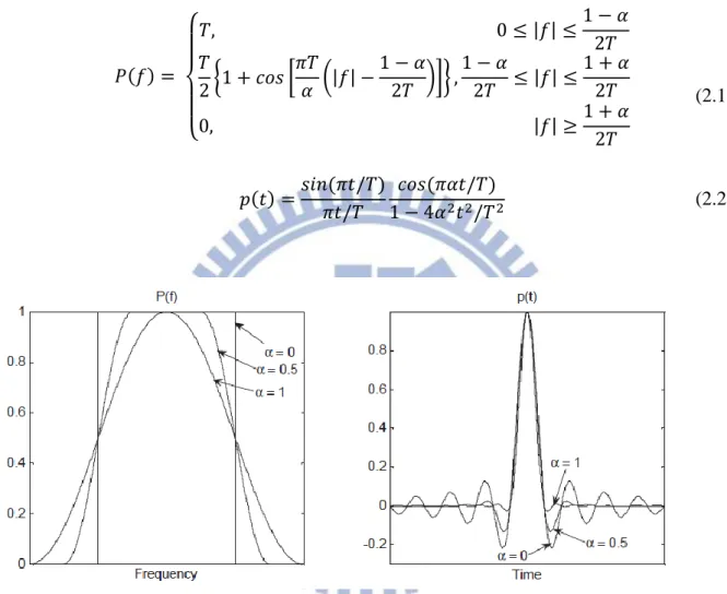
One of the commonly used pulse shaping filter is raised-cosine filter. The frequency domain and time domain representations of the filter are as follows, where T is the symbol period and α is the roll-off factor.

𝑃(𝑓) = { 𝑇, 0 ≤ |𝑓| ≤1 − 𝛼 2𝑇 𝑇 2{1 + 𝑐𝑜𝑠 [ 𝜋𝑇 𝛼 (|𝑓| − 1 − 𝛼 2𝑇 )]} , 1 − 𝛼 2𝑇 ≤ |𝑓| ≤ 1 + 𝛼 2𝑇 0, |𝑓| ≥1 + 𝛼 2𝑇 (2.1) 𝑝(𝑡) =𝑠𝑖𝑛 (𝜋𝑡/𝑇) 𝜋𝑡/𝑇 𝑐𝑜𝑠 (𝜋𝛼𝑡/𝑇) 1 − 4𝛼2_𝑡2_/𝑇2 (2.2)

Figure 2.3: Raised-cosine filter

Figure 2.3 shows the raised-cosine filter graphically in time domain and frequency domain. Roll-off factor α changes from 0 to 1 and it controls the amount of out-of-band radiation; α = 0 generates no out-of-band radiation and as α increases, the out-of-band radiation increases. In the time domain, the pulse has higher side lobes when α is close to 0 and this increases the PAPR for the transmitted signal after pulse shaping.

6

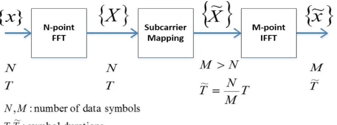
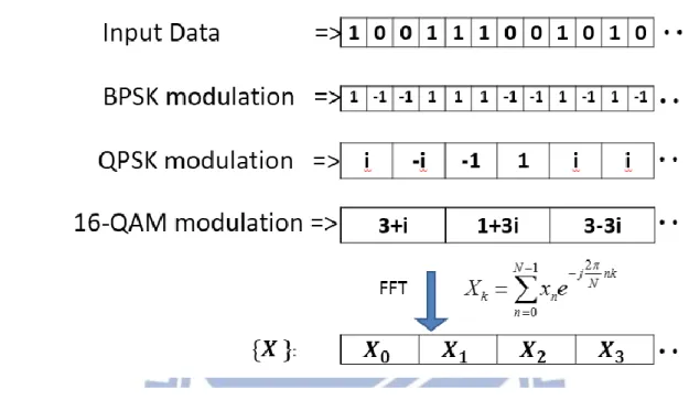
Figure 2.4: Generation of SC-FDMA transmitter symbols

Figure 2.4 details the generation of SC-FDMA transmit symbols. There are M subcarriers, among which N (<M) subcarriers are occupied by the input data. In the time domain, the input data symbol duration of T seconds and the symbol duration is compressed to 𝑇̃ = (𝑁/𝑀)𝑇 seconds after going through the SC-FDMA modulation.

The receiver retransforms the received signal into the frequency domain by FFT, de-maps the subcarriers, and then performs the frequency domain equalization. The equalized symbols are transformed back to the time domain symbols by IFFT, and data demodulations and detections are applied to get the original data.

2.2 Data modulations

There are four major classes of digital modulation techniques used for transmission, amplitude-shift keying (ASK), frequency-shift keying (FSK), phase-shift keying (PSK) and quadrature amplitude modulation. All convey data by changing some aspect of a base signal in response to a data signal. In the case of PSK, the phase is changed to represent the data signal. Two common example are “binary phase-shift keying” (BPSK) which uses two phases and “quadrature phase-shift keying” (QPSK) which uses four phases, although any number of phase may be used.

7

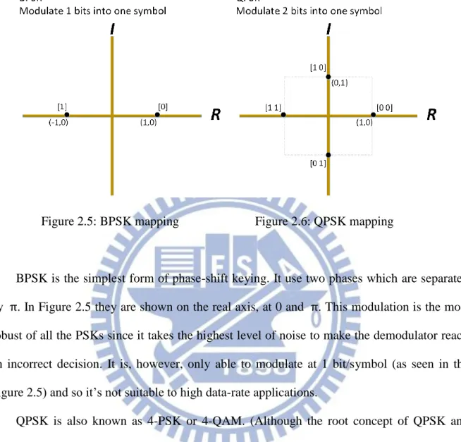
Figure 2.5: BPSK mapping Figure 2.6: QPSK mapping

BPSK is the simplest form of phase-shift keying. It use two phases which are separated by π. In Figure 2.5 they are shown on the real axis, at 0 and π. This modulation is the most robust of all the PSKs since it takes the highest level of noise to make the demodulator reach an incorrect decision. It is, however, only able to modulate at 1 bit/symbol (as seen in the Figure 2.5) and so it’s not suitable to high data-rate applications.

QPSK is also known as 4-PSK or 4-QAM. (Although the root concept of QPSK and 4-QAM are different, the resulting modulated radio wave are exactly the same.) QPSK uses four points on the constellation diagram, equispaced around the circle. With four phases, it can encode two bits per symbol, shown in Figure 2.6 with Gray coding, which encodes the data with one different bit to adjacent symbols, to minimize the bit error rate (BER). The advantage of QPSK over BPSK is that QPSK transmits the twice data rate at the same BER compared to BPSK.

8

Figure 2.7: 16-QAM and 64-QAM mapping

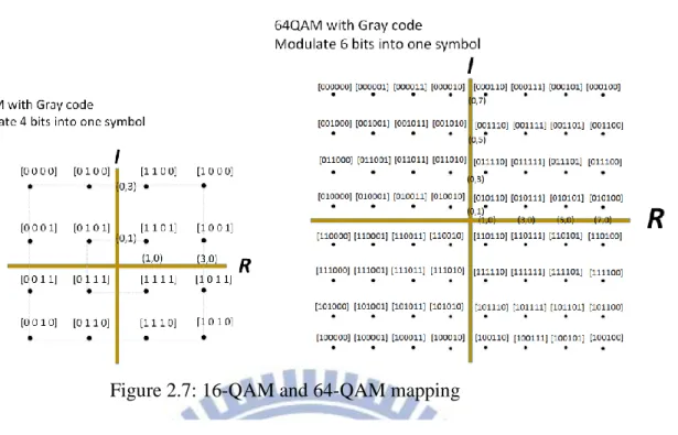
Like PSK schemes, QAM conveys data by changing some aspect of carrier signal in response to the data. In QAM, the constellation points are usually arranged in the square grid with equal vertical and horizontal spacing, although other configurations are possible (e.g. Cross-QAM). Since in digital telecommunications the data are usually binary, the number of points in the grid is usually a power of two. (e.g. 2, 4, 8, …)

The most common forms are 16-QAM, 64QAM and 256-QAM. By moving to a higher-order constellation, it is possible to transmit more bits per symbol. However, if the mean energy of the constellation is to remain the same (by way of making a fair comparison), the points must be closer together and are thus more susceptible to noise and other corruption; this results in a higher bit error rate and so higher-order QAM can deliver more data but less reliably than lower-order QAM, for constant mean constellation energy. Using higher-order QAM without increasing the bit error rate requires a higher SNR (increasing signal energy, reducing noise, or both.) If data-rates beyond those offered by 8-PSK are required, it is more usual to move to QAM since it achieves a greater distance between adjacent points in the I-Q plane by distributing the points more evenly. The complicating factor is that the points are no longer all the same amplitude and so the demodulator must now correctly detect

9

both phase and amplitude, rather than just phase. Figure 2.7 shows the 16-QAM and 64-QAM mapping with Gray coding, which can transmit 4 bits and 6 bits respectively.

Figure 2.8: Time domain symbols transform to frequency domain symbols by applying FFT.

After the data are modulated (as shown in Figure 2.8), the transmitter next groups the modulated symbols {x} into blocks each containing N symbols. Perform an N-point FFT to produce a frequency domain representation X of the input symbols. Then it maps N FFT outputs to one of the M (>N) orthogonal subcarriers.

10

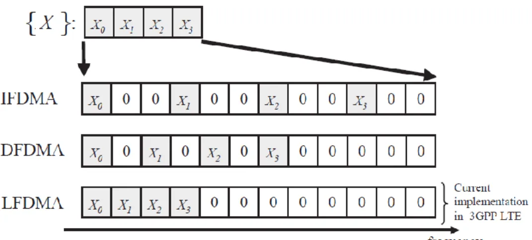
Figure 2.9: Subcarrier mapping modes

2.3 Subcarrier mapping

There are three main methods to choose the subcarriers for transmission as shown in Figure 2.9; the interleaved, distributed and localized mapping. In the interleaved subcarrier mapping mode, FFT outputs of the input data are allocated over the entire bandwidth with zeros occupying the unused subcarriers, the distributed subcarrier mapping mode is similar to the interleaved mode but it doesn’t occupy the entire bandwidth (depends on how many users at the same time), whereas consecutive subcarriers are allocated by the FFT outputs in the localized subcarrier mapping mode. We will refer to the localized subcarrier mapping SC-FDMA as LFDMA, distributed subcarrier mapping SC-FDMA as DFDMA and interleaved subcarrier mapping SC-FDMA as IFDMA.

From a resource allocation point of view, subcarrier mapping methods are further divided into static and channel-dependent scheduling (CDS) methods. CDS assigns subcarriers to the users according to the channel frequency response of each user. For both scheduling methods, distributed subcarrier mapping provides frequency diversity because the transmitted signal is spread over the entire bandwidth. By contract, the localized subcarrier mapping provides better throughput because of the significant multi-user diversity (which

11

means in a large system with independent fading of users, there is likely to be a user with a very good channel at any time.)

Figure 2.10: Subcarrier allocation methods for multiple users (3 users, 12 subcarriers, and 4 subcarriers allocated per user)

Figure 2.10 shows IFDMA and LFDMA demonstrating that the signals of three different terminals arriving at a base station occupying mutually exclusive sets of subcarriers.

2.4 Cyclic prefix insertion

Utilizing a cyclic prefix is an efficient method to prevent ISI between two successive symbols. In general, CP is a copy of the last part of the block, which is added at the start of each block for a couple of reasons.

Figure 2.11: Cyclic prefix insertion

T

M

x

x

x

M

x

M

x

L

M

x

x

[

~

[

1

],...,

~

[

2

],

~

[

1

],

~

[

0

],

~

[

1

],...,

~

[

1

]]

~

_

_

_

_

_

_

_

_(2.3)

12

1. CP acts as a guard time interval between successive blocks. If the length of CP is longer than the maximum delay spread of the channel, or roughly the length of channel impulse response, then there is no ISI.

2. Since CP is a copy of the last part of the block, it converts a discrete time linear convolution into a discrete time circular convolution. Thus transmitted data propagating through the channel can be modeled as a circular convolution between the channel impulse response and transmitted data block, which in frequency domain is a point-wise multiplication of the FFT frequency symbols. Then, to remove the channel distortion, the received signal can be simply divided by the FFT of channel frequency response point-wise or a more sophisticated frequency domain equalization technique can be implemented.

2.5 Characteristics of Wireless Mobile Communication Channel

A transmitted signal propagating through the wireless channel often encounters multiple reflective paths. We refer to this phenomenon as multi-path propagation and it causes fluctuation of amplitude and phase of the received signal. Large-scale fading represents the average signal power attenuation or path loss due to the motions over large areas. Small-scale fading is often statistically characterized with Rayleigh probability density function. Rayleigh fading in the propagation channel, which generates ISI in the time domain.

When characterizing the Rayleigh fading channel, we can categorize it into either flat fading channel or frequency-selective fading channel. Flat fading occurs when the coherence bandwidth, which is the inversely proportional to the channel delay spread, is much larger than the transmission bandwidth whereas frequency-selective fading happens when the

13

coherence bandwidth is much less than the transmission bandwidth. Two examples of the frequency response of multipath fading channel is shown in Figure 2.12.

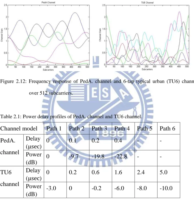
Figure 2.12: Frequency response of PedA. channel and 6-tap typical urban (TU6) channel over 512 subcarriers.

Table 2.1: Power delay profiles of PedA. channel and TU6 channel.

Channel model

Path 1

Path 2

Path 3

Path 4

Path 5

Path 6

PedA.

channel

Delay

(μsec)

0

0.1

0.2

0.4

-

-

Power

(dB)

0

-9.7

-19.8

-22.8

-

-

TU6

channel

Delay

(μsec)

0

0.2

0.6

1.6

2.4

5.0

Power

(dB)

-3.0

0

-0.2

-6.0

-8.0

-10.0

Table 2.1 illustrates the power delay profiles (PDP) of two multipath fading channel. We can create the impulse response of these channels with the PDP. The detail will be demonstrated in the simulation section.

14

2.6 Simulation

2.6.1. Simulation parameters

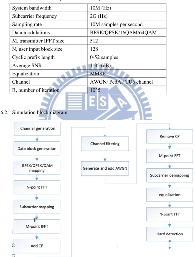
Table 2.2: Simulation parameters of Chapter 2. System bandwidth 10M (Hz) Subcarrier frequency 2G (Hz)

Sampling rate 10M samples per second Data modulations BPSK/QPSK/16QAM/64QAM M, transmitter IFFT size 512

N, user input block size 128

Cyclic prefix length 0-52 samples Average SNR 1-35 (dB) Equalization MMSE

Channel AWGN/ PedA./ TU6 channel R, number of iteration 10^5

2.6.2. Simulation block diagram

F i

g F

15

As shown in Figure 2.13, we first create R channel impulse responses and normalize the channel power. Second, produce the data symbol randomly and apply the data modulation. Collect N modulated symbols to apply N-point FFT to transform the symbol to frequency domain and map these symbol to the corresponding subcarriers. Then we apply M-point IFFT on all the subcarriers to get M transmitting symbols and add CP to cancel the effect from multipath channel.

After the transmitting symbols are produced, operate the convolution on the symbols and the channel impulse response created before and add noise.

At the receiver, it is just the reverse of the transmitter. First remove the CP from the received symbols and keep M symbols. Second, apply M-point FFT to transmit the symbols to frequency domain and demap the subcarrier. After each user achieves the corresponding frequency domain symbols, take the MMSE equalization to verify the symbols. Finally, apply N-point IFFT to transform the symbols back to frequency domain and demodulate the symbols to detect to original data

2.6.3. Simulation channel model

The impulse response of multipath fading channel is created as below, (take PedA. channel as an example)

 Create an equal strength multipath fading (Rayleigh) channel

. 0 ) 1 , 0 ( ~ , , ] ,..., , [ , ] ,..., , [ ) ( 2 1 2 1 2 1 , L i,j Ν y x y y y x x x i j i T L T L r        y x y x h_R (2.4)

16

 Multiple the square root of PDP of the PedA. channel and the h_R symbol by symbol )] ( ),..., 2 ( ), 1 ( [ _{1 , 2 , ,} ,r P Ri P Ri PL Ri L peda h h h h     (2.5)

 Finally, normalize the channel power.

Total power,







     R r r r r T L P 1 2 , 2 , 2 , (1) peda (2) ... peda ( ) peda h h h (2.6) T r r, , / P , normalized peda peda h h  (2.7)

2.6.4. Simulation added noise at receiver

 First we calculate the average power of received signal C as follow,







    R i M m m m

total real y imag y

C 1 1 2 2 ) ( ) ( (2.8) R M C C total   (2.9)

 Then we know that the CNR (carrier to noise ratio) is defined by

B R SNR B N R E N C  b b   b 0 (2.10)

Where

R

bis the channel bit rate and B is the channel bandwidth.

 So for a given SNR, we can calculate the added noise power at the receiver.

b c b c b N Q SNR C Nf N Mf SNR C R B SNR C N      (2.11)

Where

N

bis the number of bit per symbol,

Q

is the bandwidth expansion factor

17

2.6.5. Simulation MMSE frequency domain equalization The MMSE equalization matrix

W

uis given by





1 0    N H u u H u u h h h N I W (2.12)

Where H is the Hermitian transpose operation,

I

Nis the NN identity matrix

and

h

uis the NN demapped channel matrix for uth user.

2.6.6. Simulation result

18

Fiqure 2.15: BER performance of IFDMA for ideal channel

19

Fiqure 2.17: BER performance ofIFDMA for PedA. channel

20

Fiqure 2.19: BER performance of IFDMA for TU6 channel

From Figure 2.14 to Figure 2.19, the BER perfornance for four different data modulations in ideal channel, PedA. channel and TU6 channel are plotted, LFDMA and IFDMA respectively.

2.7 Conclusion of Chapter 2

In ideal channel, the BER performance in LFDMA and IFDMA are the same (as shown in Figure 2.14 and Figure 2.15) because there are no multipath fading. The frequency response of the ideal channel is a constant for all subcarriers, so the data has been transmitted over the equivalent channel frequency response for the two subcarrier mapping schemes.

As we can observe from Figure 2.14 to Figure 2.19, BPSK and QPSK have the best BER performance because they are optimal data modulations in BER performance (take the highest level of noise to make the demodulator reach an incorrect decision.) When the order of QAM

21

increases, the BER performance will degrade because of the area of decision region for each symbol become smaller.

In multipath channels (as shown in Figure 2.16 to Figure 2.19), the BER performances of IFDMA is better than LFDMA due to frequency divesity (subcarrier are not all under under bad gain). But LFDMA can provide high multiuser diversity (at least one user is under very good channel gain).

22

CHAPTER 3

PAPR REDUCTION FOR LOCALIZED SC-FDMA

3.1 Time Domain Symbol Analysis of SC-FDMA

For IFDMA, LFDMA and DFDMA, the three operations can be viewed as one linear operation on the sequence of modulation symbols {𝑋_𝑛: 𝑛 = 0,1, … , 𝑁 − 1}. Therefore each element of output sequence {𝑥̃_𝑚: 𝑚 = 0,1, … , 𝑀 − 1} is a weighted sum of the element of the input sequence, where the weights are complex numbers.

Section 3.1.1 derives the time symbols of IFDMA and also shows graphically the spectrum and time sequence of the transmitting IFDMA signal block. The formulas for the time sequences of LFDMA are more complicated than IFDMA. Section 3.1.2 shows the spectrum and time sequence of the transmitting LFDMA signals along with the formula derived.

3.1.1 Time domain symbols of IFDMA

For IFDMA, the combination of the FFT and IFFT in the transmitter is reduced to the simple signal processing operations of multiplying each input symbol by a complex number with unit magnitude repeating the input sequence with proper phase rotation Q times, where Q is the bandwidth expansion factor. The multiplication is equivalent to a rotation of each complex modulation symbol in the transmission block. To verify that this is true, we observe two properties of the FFT and its inverse: (a) equally spaced nonzero samples in one domain correspond to a periodic sequence in the other domain; and (b) a shift of r in the frequency domain corresponds to a phase rotation of each time sample. The phase rotation is accomplished by multiplying each sample by 𝑒𝑥𝑝 (𝑗2𝜋𝑟𝑚/𝑀) , where M is the number of IFFT size, r is the amount of the frequency shift, and m is the output sample index in the time

23

domain. The following paragraph is a detailed mathematical demonstration of this property. Figure 3.1 is an illustration for 𝑁 = 4 symbols per block, 𝑄 = 3 terminals and 𝑀 = 𝑄 × 𝑁 = 12 subcarriers.

For one input signal, {𝑋̃_𝑖: 𝑖 = 0,1,2, … , 𝑀 − 1} is the spectrum of the transmitted SC-FDMA sequence representing the block of data {𝑥_𝑛: 𝑛 = 0,1,2, … , 𝑁 − 1}. In IFDMA, the spectrum has M-uniformly-spaced nonzero components, with adjacent samples separated by 𝑄 − 1 samples in the frequency domain. The corresponding time domain signal {𝑥̃𝑖: 𝑖 = 0,1,2, … , 𝑀 − 1} is periodic with Q replicas distributed over time 𝑛 = 0,1,2, … , 𝑁 −

1(= 𝑀/𝑄 − 1) and with phase rotation of 𝑒𝑥𝑝 (𝑗2𝜋𝑟𝑚/𝑀). Consider the input signal {𝑥𝑛: 𝑛 = 0,1,2, … , 𝑁 − 1} that occupies subcarrier 𝑖 = 0, 𝑄, 2𝑄, … , (𝑁 − 1)𝑄. The periodic

transmitted time signal corresponding to the spread spectrum of this signal has the sequence { 𝑥₀/𝑄, 𝑥₁/𝑄, … , 𝑥_𝑁−1/𝑄}, repeated Q times. The transmitted time sequence of the signal from other terminals is similar but multiplied by phase rotation 𝑒𝑥𝑝 (𝑗2𝜋𝑟𝑚/𝑀) (due to the subcarrier mapping shift m).

24

The mathematical formulas corresponding to this description begin with the frequency domain symbols 𝑋̃_𝑖

𝑋̃𝑖 = {𝑋𝑖/𝑄_{0, otherwise} , 𝑖 = 𝑄 × 𝑘 (0 ≤ 𝑘 ≤ 𝑁 − 1) (3.1)

Where 0 ≤ 𝑖 ≤ 𝑀 − 1 and 𝑀 = 𝑄 × 𝑁

Let 𝑚 = 𝑁 × 𝑞 + 𝑛, where 0 ≤ 𝑞 ≤ 𝑄 − 1 and 0 ≤ 𝑛 ≤ 𝑁 − 1, then 𝑥̃_𝑚 = 𝑥̃_{𝑁𝑞+𝑛} = 1 𝑀 ∑ 𝑋̃𝑖 𝑀−1 𝑖=0 × 𝑒𝑗2𝜋𝑚𝑀𝑖= 1 𝑄∙ 1 𝑁∑ 𝑋𝑘 𝑁−1 𝑘=0 × 𝑒𝑗2𝜋𝑚𝑁𝑘 = 1 𝑄∙ 1 𝑁∑ 𝑋𝑘 𝑁−1 𝑘=0 × 𝑒𝑗2𝜋𝑁𝑞+𝑛𝑁 𝑘 = 1 𝑄∙ ( 1 𝑁∑ 𝑋𝑘 𝑁−1 𝑘=0 × 𝑒𝑗2𝜋𝑛𝑁𝑘) = 1 𝑄𝑥𝑛 (3.2)

The resulting time symbols {𝑥̃_𝑚} are simply a repetition of the original input symbols {𝑥𝑛} with a scaling factor in the time domain just as we derived.

When the subcarrier allocation starts from the rth subcarrier (0 < 𝑟 ≤ 𝑄 − 1), then, 𝑋̃_𝑖 = {𝑋𝑄−𝑟𝑖 , 𝑖 = 𝑄 × 𝑘 + 𝑟 (0 ≤ 𝑘 ≤ 𝑁 − 1)

0, otherwise (3.3) Corresponding to Equation (2.2), the time symbols {𝑥̃_𝑚} can be derived as

𝑥̃𝑚 =

1

𝑄𝑥𝑛∙ 𝑒𝑥𝑝 (𝑗2𝜋𝑟𝑚/𝑀) (3.4) As we can see from Equation (3.4), there is an additional phase rotation of 𝑒𝑥𝑝 (𝑗2𝜋𝑟𝑚/ 𝑀) as noted earlier when the subcarrier allocation starts from rth subcarrier instead of the first subcarrier.

25 3.1.2 Time domain symbols of LFDMA

Figure 3.2 is a diagram of the LFDMA subcarrier mapping. It shows how the modulation symbols occupy the subcarrier in the example.

Figure 3.2: Illustration of LFDMA subcarrier mapping for N=4, Q=3 M=12

The frequency domain samples after LFDMA subcarrier mapping {𝑋̃𝑙} can be derived

as follows:

𝑋̃𝑙 = {𝑋_{0, 𝑁 − 1 ≤ 𝑙 ≤ 𝑀 − 1} 𝑙, 0 ≤ 𝑙 ≤ 𝑁 − 1 (3.5)

Let 𝑚 = 𝑄 × 𝑛 + 𝑞 where 0 ≤ 𝑛 ≤ 𝑁 − 1 and 0 ≤ 𝑞 ≤ 𝑄 − 1. Then, 𝑥̃_𝑚 = 𝑥̃_{𝑄𝑛+𝑞} = 1 𝑀 ∑ 𝑋̃𝑙 𝑀−1 𝑙=0 × 𝑒𝑗2𝜋𝑚𝑀𝑙 = 1 𝑄∙ 1 𝑁∑ 𝑋𝑙 𝑁−1 𝑙=0 × 𝑒𝑗2𝜋𝑄𝑛+𝑞𝑄𝑁 𝑙 _(3.6) If 𝑞 = 0, 𝑥̃_𝑚 = 1 𝑄∙ 1 𝑁∑ 𝑋𝑙 𝑁−1 𝑙=0 × 𝑒𝑗2𝜋𝑛𝑁𝑙= 1 𝑄𝑥𝑛 (3.7) If 𝑞 ≠ 0, 𝑥̃_𝑚 = 1 𝑄∙ (1 − 𝑒 𝑗2𝜋_𝑄𝑞 ) ∙ 1 𝑁∑ 𝑥𝑝 1 − 𝑒𝑗2𝜋{𝑛−𝑝𝑁 +𝑄𝑁}𝑞 𝑀−1 𝑝=0 (3.8) Detailed derivations of equation (3.8) is derived in [7]. As we can see in Equation (3.7) and (3.8), the LFDMA signal in the time domain has exact copies of the input time domain symbols with a scaling factor at Q-multiple sample positions. Intermediate values are

26

weighted sum of all the time symbols in the input block. Figure 3.3 and Figure 3.4 show examples of the time domain symbols of IFDMA and LFDMA.

Figure 3.3: An example of IFDMA transmitting signals (M=16, N=4)

27 3.1.3 Comparison of 99.9-percentile PAPR

Figure 3.5: Time domain symbols of IFDMA and LFDMA.

It is obvious that LFDMA has higher PAPR than IFDMA because of the multiplication with complex weight in some samples. So we further compare the PAPR between OFDMA, LFDMA and IFDMA. Table 3.1 shows the comparison of 99.9-percentile PAPR, which means the probability that the PAPR is larger than the comparison value PAPR₀ is 10−3. Table 3.1: Comparison of 99.9-percentile PAPR

Mod. format IFDMA LFDMA OFDMA BPSK/QPSK 0 dB 7.5 dB 10.7 dB 16QAM 3.5 dB 8.4 dB 10.5 dB 64QAM 4.8 dB 8.7dB 10.5 dB

SC-FDMA signals indeed have lower PAPR compared to OFDMA. But when the order of QAM (number of bit per symbol) increases, the advantage in PAPR of LFDMA compared to OFDMA becomes less and less. So in the rest of this chapter, we investigate a common method used in reducing PAPR, selective mapping (SLM)m a proposed feedback-searching SLM and proposed symbol-replaced methods.

28

3.2 Basic SLM for PAPR Reduction

3.2.1 Block diagram of basic SLM

Figure 3.6: Block diagram of basic SLM for SC-FDMA system-transmitter

Figure 3.7: Block diagram of basic SLM for SC-FDMA system-receiver

Figure 3.6 and 3.7 show the block diagrams of the transmitter/receiver of basic SLM for SC-FDMA system. In LFDMA, the transmitting time domain sequence is 𝑥̃_𝑚 which is derived in the Section 3.1.2, so the PAPR of the transmitted sequence can be defined as

PAPR =max (|𝑥̃𝑚|2) 𝐸[|𝑥̃𝑚|2]

29 3.2.2 Formulation of basic SLM transmitter

At the transmitter, as seen in Figure 3.6, the input data d for a particular user can be expressed by T

d[N]]

d[2],....,

[d[1],



d

(3.10)

And there are U different phase shift vectors that transmitter and receiver both know.

T u N u N u u u u

P

C

P

C

P

C

,

,...,

]

[

_{1 1 2 2} u



P

(3.11) Where_Pu _e vu v 

 and



_vuis uniformly distributed in(0,2)for

v

=1,2,…,N and

u

=1,2,…,U. . and on depend 1 v u C_vu     C

We get U different sequences by bitwise multiplied U different phase shift vectors.

T u N u N u u u u

P

C

P

C

P

C

d[1]

,

d[2]

,...,

d[N]]

[

_{1 1 2 2} u u







d

d

P

(3.12)

Where 0uU (donates thebitwisemultiplication)

Then each sequence apply N-point FFT.

T u N u N u u u u u

P

C

P

C

P

C

d[1]

,

d[2]

,...,

d[N]]

[

_{1 1 2 2} N u N

d

F

F

X





(3.13)

And followed by subcarrier matrix multiplication. (Gis themappingmatrix)

u

GX

X~u  (3.14)

Transform the symbols to the transmitting time domain symbols.

u 1

~

~

_x

_

_F



_X

M

u _(3.15)

Then select the lowest PAPR sequences ~_xumin_{from U sequences.}

] d[N]] ,..., d[2] , d[1] [ [ ~ ~ min min min min min min min min 2 2 1 1 1 1 T u N u N u u u u N M u M u P C P C P C F G F X F x     (3.16)

30 3.2.3 Side information

In our thesis, we use a SLM technique that allows for SI index u to be embedded in the transmitted data so that no additional bits need to be sent to the receiver. In this method, the coefficient of K elements of the phase shift vector are set to a constant C > 1, called extension factor, whereas the moduli of the other (N-K) elements remain equal to the unit. To allow for SI recovery in the receiver, there must be a one-to-one correspondence between an index u and a set of C value positions. The number of distinct sets that can be generated is given by the binomial coefficient

)! ( ! ! K N K N K N        

. Figure 3.8 shows an example that it uses two different positions to index 10 different phase shift vectors.

In the receiver, it measures the amplitude of the time domain data symbols and the end of N-point IFFT and estimate the index the phase shift vector that C positions indicate. Then we can divide the right phase shift vector to recover the original data.

31

3.3 Proposed Feedback-Searching SLM for PAPR Reduction

3.3.1 Block diagram of proposed feedback-searching SLM

Figure 3.9: Block diagram of the proposed SLM for SC-FDMA system-transmitter Figure 3.9 shows the block diagrams of the transmitter of the proposed

feedback-searching SLM for SC-FDMA system and the receiver is the same with the basic one (as shown in Figure 3.7).

3.3.2 Algorithm for the proposed feedback-searching SLM

Algorithm Proposed feedback-searching SLM

1. Apply the SLM in the first step with 1 phase shift vector.

2. Record the PAPR as the minimum PAPR at the end of M-point IFFT.

3. Then modify the phase shift factor by multiplying –C one by one and compared with the minimum PAPR. If the modified one is smaller, update the minimum PAPR and corresponding phase shift factor.

4. Repeat step 3 until all phase shift factors are searched, then transmit the signal with the smallest PAPR

32

3.3.3 Comparison of computation complexity with basic SLM

Table 3.2: Comparison of computation complexity with two SLMs

Method Multiplication numbers Data statistic M=512, U=128 N=128 M=512, U=256 N=256 SLM M M U N N U N U log log      720896 1769472 FS-SLM M M U N N U N log log 3      704768 1704448

Table 3.2 shows that the number of computation of FS-SLM is slightly lower than the basic SLM because that the difference of multiplications before the N-point FFT. The basic SLM takesUNsymbol-wise multiplications and the FS-SLM takes2N symbol-wise multiplications and additionalN comparison at the end of M-point IFFT.

3.4 Symbol-Replaced method for PAPR Reduction(practical)

3.4.1 Block diagram of the symbol-replaced method

33

Figure 3.10: Block diagram of symbol-replaced method for SC-FDMA system-receiver

Figure 3.9 and Figure 3.10 shows the block diagram of transmitter and receiver of the symbol-replaced method. In the transmitter, it is very similar to the basic SLM except for the beginning of the N-point FFT. The detail algorithm will be derived in section 3.4.2.

3.4.2 Algorithm for the symbol-replaced method

Figure 3.11: An example of the symbol-replaced method. (B=5)

Algorithm Symbol-replaced method-transmitter

1. Define B as the number of symbols to be replaced by random phase sequences. 2. Generate U random phase sequence with length B

3. Add random phase sequence in front of (N- B) input data parallelly before they go through the N-point FFT.

4. After U sequences go through all the operations, select the lowest PAPR sequences to transmit.

34 Algorithm Symbol-replaced method-receiver

1. When we receive the data from channel, apply the M-point FFT, subcarrier demapping, frequency domain equalization and N-point IFFT just like regular SC-FDMA processing.

2. Abandon first B symbols directly.

3. Detect the rest of symbols without any sequence multiplications.

3.4.3 Improved feedback-searching symbol-replaced method

Figure 3.12 Block diagram of Feedback-searching symbol-replaced method for SC-FDMA system-transmitter

Figure 3.12 shows the transmitter of block diagram of feedback-searching symbol-replaced method and the receiver is the same with the symbol-replaced method as shown in Figure 3.10.

35

Algorithm Feedback-searching symbol-replaced method

1. Apply the symbol-replaced method in the first step with 1 random phase sequence. 2. Record the PAPR as the minimum PAPR at the end of M-point IFFT.

3. Then modify the phase shift factor by multiplying j2 m/(K1)

e  from m=1,…,K. (K is the number of searching phases per symbol) one by one and compared with the minimum PAPR. If the modified one is smaller, update the minimum PAPR and corresponding phase shift factor.

4. Repeat step 3 until all phase shift factors are searched, then transmit the signal with the smallest PAPR

3.5 Simulation

3.5.1 Simulation parameters

Table 3.3: Simulation parameters of Chapter 3. Data modulation format BPSK Subcarrier mapping Localized M, Transmitter IFFT size 512

N, User input block size 64/128/256 U, the number of phase shift vectors 128/258

Channel AWGH/ PedA channel R, number of iteration 10^5

36 3.5.2 Simulation results

Figure 3.13: The BER performance of two different symbol-replaced methods

37

Figure 3.15: The BER performance of basic SLM over different C values.

38

Figure 3.17: The BER performance of different PAPR reduction methods over different SNR values in ideal channel.

Figure 3.18: The BER performance of different PAPR reduction methods over different SNR values in PedA. channel.

39

3.6 Conclusion of Chapter 3

There are many methods to reduce the PAPR of transmission signals. We here choose the SLM as reference because the complexity of those methods are similar are the side information can be easily embedded in the signals.

Proposed SLM performs feedback searching instead of selecting from random phase shift vectors. It searches the phase symbol by symbol to ensure that the PAPR will be better and better when the phase is modified.

When the extension factor 𝑪 increases, the BER will decreases because it is easier to detect the position of 𝑪 values such that the index of phase shift vectors can be indicate. But there is a limit on the BER performance when 𝑪 increases because 𝑪 will also enhance the noise which will affect the data detection of the original data.

Though Symbol-replaced method doesn’t perform better in PAPR reduction compared to those two SLM reduction methods, it is a reliable method in transmission because it doesn’t need to detect side information. So the BER performance will not be affected by the detection error of the side information

40

CHAPTER 4

RESOURCE ALLOCATION IN LTE UPLINK

4.1. System Model and Transmission Schemes

Figure 4.1: Block diagram of the whole SC-FDMA system

41

The figure 4.1 shows that all users transmit their data over the same frequency resource simultaneously, but the key that those signals from different users will not interfere each other because they map the frequency domain symbols to the allocated subcarriers and transmit a null value on the subcarriers that are not allocated to it, leaving them to be used by other users. (as shown in Figure 4.2)

4.2. Problem Formulation

Assumption

1. Each user is matched to exactly one resource block, which consist of 1 or more subcarriers.

2. All users require the same rate and have the same power requirement.

The aim of dynamic resource block allocation is to give the user channel resource such that the performance of the whole system (as overall BER is concerned) will be optimized.

First we define the gain matrix C is given by

             UK U K K c c c c c c       1 2 21 1 11 C (4.1) ly. respective RBs and users of number the are and whereU K U u K k h c kN )N (k n un uk 1: and 1: 1 1    



   (4.2) u un u h u k H matrix channel s user' th from elements diagonal the are and index user the is index, RB the is where

42

And our goal is to maximize the utility function below to achieve the best performance for the whole system.



   U u K k uk uk c c s J 1 1 (4.3) ) 0 otherwise , user to allocated is RB when 1 ( . matrix choice he t of elements the are and matrix gain the of elements the are where   uk uk uk uk s u k s s c S C

4.3. Greedy Method

Algorithm Greedy method

1. Define 𝐾 as the set of unassigned resource blocks.

2. Start from the first user, search the gain in gain matrix C to each resource block in 𝐾. Find the resource block with the highest gain and assign the resource block to this user. 3. Remove the resource block from 𝐾.

4. Move on to the next user and perform steps 2 to 3 again, until all the users have been allocated a resource block.

Figure 4.3: A simple example of greedy method

In Figure 4.3, the user from the first to the last searches the highest gain from the corresponding row of the gain matrix to allocate the resource block.

43

4.4. Maximum Greedy Method

Algorithm Maximum greedy method

1. First define different solution spaces (the user priority of applying the Greedy Method). 2. For each unique solution space, perform the greedy algorithm in Section 3.3 and save the

solution.

3. Find the best one from saved greedy solutions.

Figure 4.4: A simple example of maximum greedy method

In Figure 4.4, there is an example that allocate the resource block to the user from the last to the first (another solution space) and searches the highest gain from the corresponding row of the gain matrix to allocate the resource block.

44

4.5. Proposed BER-Enhanced Greedy Method

Algorithm Maximum greedy method

1. Define 𝑼 as the set of all unallocated users and 𝑲 as the set of unassigned RBs. 2. Calculate the total channel gain of user 𝑢 for all users in 𝑼.

𝑚𝑢 = _‖𝐾‖1 ∑ 𝑐𝐾 𝑢𝑘, ∀𝑢 ∈ 𝑼

3. Find the user 𝑢̃ with smallest total channel gain, and then search the highest gain 𝑐_𝑢̃𝑘̃ from the corresponding row of the gain matrix 𝑪 .

4. Then assign the resource block 𝑘̃ to the user 𝑢̃ and remove this RB from 𝑲. 5. Remove user 𝑢̃ from 𝑼

6. Repeat step 2 to 5 until 𝑼 ∈ ∅

Figure 4.5: A simple example of BER-enhanced greedy method

In Figure 4.5, the resource block assignment starts from the user with smallest total channel gain and assign the highest RB to the user, then followed by the second smallest until all users are allocated a RB.

45

4.6. Comparison of Computation among these three methods

Table 4.1: Comparison of computation complexity among these three methods. (assume U=K, the number of user is the same with the number of resource block)

Algorithm # of Computation Complexity Greedy method ∑(𝑘 − 1) =

𝐾 𝑘=1

1

2𝐾(𝐾 − 1) 𝑂(𝐾2)

Maximum greedy method 𝑎 ∑(𝑘 − 1) =

𝐾 𝑘=1

𝑎

2𝐾(𝐾 − 1) 𝑂(𝑎𝐾2)

BER-enhanced greedy method ∑(𝑘2+ 𝑘 − 2) =

𝐾 𝑘=1 1 3𝐾3+ 𝐾2− 4 3𝐾 𝑂(𝐾3) Where 𝒂 is the number of solution space.

Table 4.1 illustrates the computation complexity of these three methods. For the greedy method, it takes K-1 comparisons to find the highest gain for the first user and linearly decreasing by 1 for assigning each user a resource block. It is clearly that the total computations is ∑𝐾_𝑘=1(𝑘 − 1). For the maximum greedy method, it simply a times of the greedy method. For the BER-enhanced method to find the first user to assign a RB, we need to calculate the total gain (takes K-1 computations) of K users and find the one with smallest total gain (takes K-1 computations). And then find the highest gain (takes K-1 computations) of the user to allocate a RB. So the total number of computation can be derived as ∑𝐾_𝑘=1(𝑘2+ 𝑘 − 2).

46

4.7. Simulation

4.7.1. Simulation parameters

Table 4.2: Simulation parameters of Chapter 4. System bandwidth 10M (Hz) Subcarrier frequency 2G (Hz) Data modulation format BPSK M, Transmitter IFFT size 512 SNR 1-30 (dB)

U, Number of users 4/8/16/62/64/128/256 Equalization MMSE

Multipath fading channel PedA. channel Number of iteration 10^6

4.7.2. Simulation results

47

Figure 4.7: The effect on BER performance for different number of users

4.8. Conclusion of Chapter4

BER-Enhanced Greedy Method has better performance in BER because the algorithm is to find a solution space that can enhance the BER performance, but not necessarily better in total system throughput (or other performance of the whole system).

There is a trade-off between the quality of the solution and the complexity. This is very intuitive that if we spend more computation to compare and choose the better solutions.

For these three greedy methods, when the number of users increases, the BER performance will be better because the channel will be divided into smaller resource blocks. So resource blocks can be allocated better according to the channel.

48

REFERENCES

[1] 3rd _{Generation Partnership Project, Technical Specification Group Radio Access}

Network; Physical layer aspects for evolved Universal Terrestrial Radio Access (UTRA), 3GPP Std. TR 25.814 v7.0.0.

[2] Islam M.R. , Irfan M., Ullah N., Ullah S., Fahim S.M. and Azad I.I. ,” Non Binary SC-FDMA for 3GPP LTE uplink”, Computing, Communications and Applications Conference (ComComAp), p198-203, Oct. 2012 .

[3] de Temino L. , Berardinelli Gilberto, Frattasi S., Pajukoski K. and Mogensen P. ,” Single-user MIMO for LTE-A Uplink: Performance evaluation of OFDMA vs. SC-FDMA”, Radio and Wireless Symposium, 2009. RWS '09. IEEE, pp. 304-307, 2009 .

[4] H. G. Myung, J. Lim and D. J. Goodman, “Single carrier FDMA for uplink wireless Transmission ,” Vehicular Technology Magazine, IEEE ,pp.30-38, Sep. 2006.

[5] H. G. Myung, J. Lim and D. J. Goodman, “Peak-to-Average Power Ratio of Single Carrier FDMA Signals with Pulse Shaping,” Proc. Of the IEEE PIMRC, pp.1-5 Sep. 2006.

[6] Mohammad A., Zekry A. and Newagy F.,”A Time Domain SLM for PAPR reduction in SC-FDMA Systems,” Global High Tech Congress on Electronics (GHTCE), 2006 IEEE, pp. 143-147, 2006.

[7] St´ephane Y. Le Goff, Samer S. Al-Samahi, Boon Kien Khoo, Charalampos C. Tsimenidis, and Bayan S. Sharif, “Selected Mapping without Side Information for PAPR Reduction in OFDM,” IEEE TRANSACTIONS ON WIRELESS COMMUNICATIONS, VOL. 8, NO. 7, JULY 2009

[8] Lu Xuan-min, WangYu-shiand ZhouYa-jian,“An Improved SLM Algorithm for PAPR Reduction in OFDM,” Information Engineering (ICIE), 2010 WASE International, pp.69-72, 2010.

[9] Wang Wen-Bo and Zheng Kan, “The OFDM Technique of broadband wireless,” Beijing, Post and Telecom press, 2003.

[10] Miao Wang, Zhangdui Zhong, Qiuyan Liu, ”Resource Allocation for SC-FDMA in LTE Uplink,” Service Operations, Logistics, and Informatics (SOLI), 2011 IEEE International Conference, pp.601-604, 2011.

49

[11] Shibata K. , Webber J., Nishimura T., Ohgane T., Ogawa, Y. ,” Blind Detection of Partial Transmit Sequence in a Coded OFDM System”, Global Telecommunications Conference, 2009. GLOBECOM 2009. IEEE, pp.1-6

[12] Robert J. Baxley and G. Tong Zhou,” Comparing Selected Mapping and Partial Transmit Sequence for PAR Reduction”, IEEE TRANSACTIONS ON BROADCASTING, VOL. 53, NO. 4, DECEMBER 2007

[13] Leonard J. Cimini, Jr. and Nelson R. Sollenberger, “Peak-to-Average Power Ratio Reduction of an OFDM Signal Using Partial Transmit Sequences” IEEE

COMMUNICATIONS LETTERS, VOL. 4, NO. 3, MARCH 2000

[14] Keunyoung K., Hoon, K., Youngnam, H. and Seong-Lyun, K., “Iterative and greedy resource allocation inan uplink OFDMA system” in proc. 15th IEEE International

Symposium on Personal, Indoor and Mobile Radio Communications, PIMRC, Barcelona,

Spain,September, 2004, pp. 2377-2381.

[15] Junsung Lim ,Myung, H.G. ; Kyungjin Oh ; Goodman, D.,” Channel-Dependent Scheduling of Uplink Single Carrier FDMA Systems”, Vehicular Technology Conference, 2006. VTC-2006 Fall. 2006 IEEE 64th

[16] Hyung G. Myung and David J. Goodman, Single Carrier FDMA A New Air Interface for Long Term Evolution, first edition, John Wiley & Sons, Ltd., United Kingdom, 2008.