即時的積分直方圖基準之聯合雙邊濾波演算法分析與設計

國 立 交 通 大 學

電子工程學系 電子研究所碩士班

碩 士 論 文

即時的積分直方圖基準之聯合雙邊濾波演算法分析與設計

Analysis and Design of Real-time Integral Histogram Based

Joint Bilateral Filtering

研究生︰許博雄

指導教授︰張添烜 博士

即時的積分直方圖基準之聯合雙邊濾波演算法分析與

設計

Analysis and Design of Real-time Integral Histogram Based

Joint Bilateral Filtering

研 究 生︰許博雄 Student: Po-Hsiung Hsu 指導教授︰張添烜 博士 Advisor: Dr. Tian-Sheuan Chang

國 立 交 通 大 學 電子工程學系 電子研究所碩士班

碩 士 論 文

A Thesis

Submitted to Department of Electronics Engineering & Institute of Electronics College of Electrical and Computer Engineering

National Chiao Tung University in Partial Fulfillment of the Requirements

for the Degree of Master of science in

Electronics Engineering August 2010

Hsinchu, Taiwan, Republic of China

即時的積分直方圖基準之聯合雙邊濾波演算法分析與

設計

研究生: 許博雄 指導教授: 張添烜 博士 國立交通大學 電子工程學系電子研究所碩士班

摘 要

雙邊濾波演算法和聯合雙邊濾波演算法已經被廣泛運用在許多影像處理的 領域中，例如去除雜訊、色調處理、甚至是立體的相關應用和 MPEG 標準。它 雖然可以用快速演算法中的積分直方圖方法加速，但針對需要即時處理的應用， 仍然遭受高運算複雜度，高記憶體使用量的問題。要解決這些問題，VLSI 實現 是個必要的方法。本篇研究針對積分直方圖基準之(聯合)雙邊濾波演算法提出一 個有效率的硬體架構，其中包含三個自提的記憶體減量方法和可大量平行運算的 單元。 這些自提的記憶體減量方法包含動態更新方法，條狀切割方法，和積分起點 位移方法。其中動態更新方法是在運算期間，利用演算法循序逐列掃描計算的特 性，移除不再使用的資料。而條狀切割方法則進一步將每一張畫面切割成許多縱 向的條狀區域並作為逐列掃描計算的單位；每個條狀區域的寬度比畫面寬度短得 多，因此逐列掃描計算只需通過較短的列長，使得資料暫存量大減，不再需要整 個畫面寬的記憶體空間。最後，積分起點位移方法利用循序 動 態 積 分 起 點 的概念，協助原始直方圖演算法的積分過程減少對儲存資料的依賴，使得記憶體 使用量得以由整張畫面的尺度，減少至列的尺度。整體來說，這三個方法很容易 i

結合起來，可以將記憶體使用量減少至原演算法的 0.003%。 另一方面，自提的硬體架構利用延遲暫存資料共用方法和使用查表選擇器， 分別解決了積分直方圖運算上高頻寬需求和大量查表的問題;並且利用記憶體的 切割來提升內部頻寬的容量。除此之外，它也使用數值(在影像中則為亮度)空間 平行方法來有效率地執行大量積分直方圖單元運算，而達到高產出。另外，這個 硬體架構的運算模組佈局與參數的選擇無關，因此對於不同參數需求的應用，將 不需再重新設計。 最後的硬體實現，在聯華電子 90 奈米製程下，使用 200 MHz 的工作時脈， 每秒可以執行 60 張 HD1080p (1920x1080)影像。晶片總共需要 355 K 個邏輯閘和 23 K 個晶片記憶體。 ii

Analysis and Design of Real-time Integral Histogram Based

Joint Bilateral Filtering

Student: Po-Hsiung Hsu Advisor: Tian-Sheuan Chang

Department of Electronics Engineering & Institute of Electronics National Chiao Tung University

Abstract

Bilateral filtering and joint bilateral filtering have been widely used in many image processing fields, such as de-noising, tone-management, and even the 3-D applications and MPEG standard. They can be accelerated by the associated fast algorithm, integral histogram, but still suffer from highly computational complexity and massive memory, especially for real-time applications. To conquer them, VLSI implementation becomes a necessary solution. In the thesis, we design an efficient hardware architecture, which consists of three proposed memory reduction methods, and highly parallel computational components for integral histogram based (joint) bilateral filtering.

The proposed memory reduction methods include runtime updating method (RUM), stripe-based method (SBM), and sliding origin method (SOM). The RUM in runtime takes advantage of progressive raster-scan process of computation to discard unnecessary data. The SBM further divides each frame into vertical stripes and processes them one by one. These stripes are much narrower than a frame; therefore, the raster scan process can traverse along shorter rows and the original frame-wide

memory cost can be significantly reduced. Finally, the SOM uses the concept of progressive sliding integral origin to help the original histogram integration process lessen the dependency on storage data; therefore, the memory requirement can be reduced from frame-scale-magnitude to line-scale-magnitude. On the whole, the three methods can be easily combined to reduce the memory cost to 0.003% of the original requirement.

On the other hand, the proposed hardware architecture solves the integral histogram computational high bandwidth and large table problem by using delay-buffer data-reuse method and table selector, respectively. And use memory banks to enlarge the capacity of internal memory bandwidth. Besides, it uses range (intensity, for image)-space-parallelism methods to process large amount of histogram bins simultaneously to achieve high throughput. What’s more, the function block layout of the hardware architecture is invariant to parameter selection; therefore, it doesn’t have to be redesigned for applications of different parameter demands.

The final design implemented by UMC 90nm CMOS technology can achieve 60 frames per second for HD1080p (1920x1080) resolution image under 200MHz clock rate. The chip consumes 355 K gate counts and 23 K Bytes on-chip memory.

 

誌 謝

首先，要感謝我的指導教授—張添烜博士，在研究和修課上讓我能夠自由的 發揮；不管是研究本身或是工作應徵，在我遇到瓶頸都給予適切的建議與協助， 讓我得以用正確且有效率的方式來解決問題。老師良師益友的形象，深植我心。 此外，實驗支援研究的軟硬體充足，電腦設備操作環境寬敞，光線充足；讓我有 個舒適的研究環境。 感謝我的口試委員們，清華大學資訊工程系邱瀞德教授與交通大學電子工程 系王聖智教授。感謝你們百忙之中抽空前來指導，因為教授們的寶貴意見，讓我 的論文更加的充實而完備。 接著我要感謝實驗室的好夥伴們，特別是引我入門的曾宇晟學長，從零開始 帶我進入立體相關應用的領域；不斷提供並分析可行的方向；並指導我論文寫作 的技巧。也感謝林佑昆，張力中和李國龍等學長經驗的傳承，讓我受用無窮。謝 謝蔡宗憲學長，上班之後百忙中還能撥空協助我完成計畫。謝謝陳之悠學長曾力 薦我加入該實驗室。也謝謝王國振，許博淵，沈孟維，蔡政君等學長和黃筱珊學 姊曾經提供我研究上寶貴的經驗和協助。接著謝謝在國科會計畫中鼎力相助的洪 瑩蓉以及吳英佑學弟，沒有你們的即時幫忙，我恐怕無法順利 demo。謝謝 IC 競 賽戰友陳奕均，一起硬拼 12 小時拿下佳作，真的很難忘。也謝謝買飯團固定班 底廖元歆和陳宥辰，讓我天天不用孤單的走向二餐。此外，實驗室的邱亮齊，溫 孟勳，曹克嘉學弟也不能忘，是我平日一起經歷歡笑的好夥伴。 特別感謝生了病卻還不斷為我論文掛心提醒的媽媽，並祈求她早日康復。並 感謝永遠支持我的家人們：我的爸爸、弟弟，還有一直陪伴在旁替我加油的女友， 你們的支持與鼓勵，是我順利完成學業的最大動力。 在此，謹將本論文獻給所有愛我以及我愛的人。 v

Contents

1.

 

Introduction ... 1

 

1.1.  Background ... 1 

1.2.  Motivation and contribution ... 2 

1.3.  Thesis Organization ... 2 

2.

 

Introduction of Bilateral Filtering ... 3

 

2.1.  Overview ... 3 

2.2.  Bilateral Filtering ... 3 

2.3.  Application ... 8 

2.3.1.  De-noising ... 8 

2.3.2.  Texture and illumination separation ... 9 

2.3.3.  Joint Bilateral Filtering ... 10 

2.4.  Summary ... 11 

3.

 

Related Work ... 12

 

3.1.  Support-pixel-first Approach ... 14 

3.1.1.  Piece-wise linear algorithm and Yong’s algorithm ... 14 

3.1.2.  Bilateral grid ... 15 

3.2.  Target-pixel-first Approach ... 16 

3.2.1.  Separable algorithm ... 17 

3.2.2.  Histogram & Huang’s algorithm ... 17 

3.2.3.  Weiss’ Distributed Histogram ... 19 

3.2.4.  Integral Histogram ... 20 

3.3.  Summary ... 22 

4.

 

Analysis of Integral histogram based JBF ... 23

 

4.1.  Integral histogram based JBF ... 24 

4.2.  Design Challenge ... 26 

4.2.1.  High Memory Cost for integral histograms ... 28 

viii

4.2.2.  High Computational Complexity in All Processes ... 28 

4.2.3.  High Bandwidth in Integration and Extraction ... 29 

4.2.4.  Large Range Table in Kernel Calculation ... 29 

4.3.  Summary ... 29 

5.

 

Proposed Memory Reduction Methods ... 31

 

5.1.  Overview ... 31 

5.2.  Runtime Updating Method (RUM) ... 31 

5.3.  Stripe Based Method (SBM) ... 33 

5.4.  Sliding Origin Method (SOM) ... 36 

5.5.  Combination ... 39 

5.6.  Comparisons ... 40 

6.

 

Architecture Design and Implementation ... 41

 

6.1.  Overview ... 41 

6.2.  Overall architecture ... 43 

6.3.  Interface.. ... 44 

6.4.  Time Schedule ... 46 

6.5.  Design Components ... 47 

6.5.1.  Histogram Calculation Engine ... 47 

6.5.2.  Convolution Engine ... 52 

6.5.3.  Parameters versus hardware cost ... 54 

6.5.4.  Summary to design components ... 55 

6.6.  Memory Cost Analysis ... 56 

6.7.  Implementation Result ... 57 

7.

 

Conclusion ... 60

 

List of Figures

Fig. 2.1. Illustration of space kernel f and range kernel g of BF ... 4 

Fig. 2.2. Smoothing Results ... 5 

Fig. 2.3. Gaussian kernel’s bandwidth ... 6 

Fig. 2.4. Smoothing results of BF with different range parameter σr ... 7 

Fig. 2.5. Flow of flash and no-flash image correction [10] ... 9 

Fig. 3.1. Classification of acceleration approaches ... 12 

Fig. 3.2. Concept of histogram-based approaches ... 18 

Fig. 3.3. Concept of Huang’s algorithm ... 18 

Fig. 3.4. Concept of Weiss distributed Histogram: ... 20 

Fig. 3.5. Three-tier hierarchical distributed Histogram [33] ... 20 

Fig. 3.6. Concept of integral histogram ... 20 

Fig. 4.1. Concept of integral histogram approach ... 25 

Fig. 4.2. Analysis of Design Challenges over frame resolutions ... 27 

Fig. 5.1. Runtime updating method (RUM) ... 32 

Fig. 5.2. Stripe based method (SBM) ... 33 

Fig. 5.3. Integral region of SBM is an extended stripe. ... 33 

Fig. 5.4. Overlapped integration region between two adjacent stripes ... 34 

Fig. 5.5. Sliding Origin Method (SOM) ... 36 

Fig. 5.6. Sliding Origin Method ... 38 

Fig. 5.7. Combination of memory reduction methods ... 39 

Fig. 6.1. Proposed architecture of JBF ... 43 

Fig. 6.2. Mechanism of input and output data control ... 44 

Fig. 6.3. Process of Ping-Pong Structure ... 45 

Fig. 6.4. Schedule of the proposed architecture ... 46 

Fig. 6.5. Selected-bin adder in the histogram calculation engines ... 48 

Fig. 6.6. Architectures of histogram calculation engines h’c and hc ... 48 

Fig. 6.7. The delay-buffer method ... 49 

Fig. 6.8. On-chip memory with even bank and odd bank ... 50 

Fig. 6.9. Schedule phases of on-chip memory ... 50 

Fig. 6.10. Proposed architecture ... 52 

Fig. 6.11. Construction of constant weight table ... 52 

Fig. 6.12. Analysis of Hardware performance and memory reduction ... 56 

x

List of Tables

TABLE. 3-1 Comparison of computational complexity and memory cost in

related work ... 13 

TABLE. 4-1 Computational flow and complexity analysis for each pixel in the integral histogram based JBF ... 24 

TABLE. 5-1 Comparisons of original and reduced memory cost ... 40 

TABLE. 6-1 Modified computational flow and complexity analysis for each pixel in the integral histogram approach for JBF ... 41 

TABLE. 6-2 Parameters and their associated engine components ... 54 

TABLE. 6-3 Example implementation result of the proposed architecture ... 58 

TABLE. 6-4 Comparison of hardware cost per frame ... 59 

1. Introduction

1.1. Background

Bilateral filtering [1] is a special image smoother which can remove small-scale texture or noise while preserving large-scale structure or edges. The judgment to be noise or edge could be determined by an easy-tuning parameter. The ability of easily separating small-scale and large-scale contents makes bilateral filtering be more widely used than a typical smoother, such as joint bilateral filtering. Joint bilateral filtering, which is a variety of bilateral filtering combined with a guidance concept, is associated with more widely applications such as up-sampling [2], adaptive support weight [3], and even 3-D related processing [4] and MPEG standard [5].

The challenge of real time implementation for bilateral filtering is the high computational complexity of its window processing. Many algorithms have been proposed to reduce the complexity. In the thesis, we category them into two approaches: support-pixel-first approach and target-pixel-first approach. In previous work, the support-pixel-first approach was implemented through GPU programming, and achieved real-time speed. However, GPU hardware is general purpose platform and not a dedicated low-cost implementation for embedded applications. Therefore, VLSI hardware implementation is a better solution to minimize hardware cost and achieve real-time speed.

For VLSI hardware implementation, the support-pixel-first approach requires a frame-scale-magnitude memory, but it can not be reduced because of its iterative process by frames. On the other hand, the target-pixel-first approach also suffers from

frame-scale-magnitude memory requirement. Nevertheless, the cost is likely to be reduced since its progressive process with pixel-by-pixel order.

1.2. Motivation and contribution

Motivated by the high memory cost in joint bilateral filtering, this thesis proposed efficient hardware architecture based on integral histogram algorithm of the target-pixel-first approach. The goal is to build a dedicated hardware for low memory cost real-time joint bilateral filtering.

The major contributions of this thesis are three.

1. Based on integral histogram based joint bilateral filtering, we proposed three memory reduction methods to significantly reduce the memory cost. This makes integral histogram based joint bilateral filtering suitable for simpler on-chip memory based implementation in ASIC.

2. We propose an efficient hardware architecture which can efficiently process parallel operations and achieve high throughput.

3. We implemented the low memory cost real-time hardware of the proposed architecture with the three proposed memory reduction methods.

1.3. Thesis Organization

Chapter 2 briefly introduces bilateral filtering and its applications. Chapter 3 introduces the acceleration algorithms for bilateral filtering. Chapter 4 discusses the design challenges of integral histogram based joint bilateral filtering. To solve these challenges, Chapter 5 proposes three proposed memory reduction methods, and Chapter 6 proposes an efficient hardware architecture. Finally, Chapter 7 gives the conclusion of this thesis.

2. Introduction of Bilateral Filtering

2.1. Overview

Bilateral filtering (BF) is primary adopted in image processing for de-noising. With BF’s de-noising (or smoothing), the object edges and borders of image are preserved. As a result, BF becomes popular because it can provide a no-blur clear result. Moreover, the edge-preserving capability enables us to adapt BF for many advanced applications such as texture editing, tone management, demosaicing, stylization, and optical flow estimation [6].

2.2. Bilateral Filtering

BF, originated by Tomasi and Manduchi [1], is defined as,

(

)

(

)

(

)

(

)

∑

∑

∈ ∈ − − − − = S q c q S q c q q c I I g q c f I I I g q c f I BF )( , (2.1)

where c is the target pixel, and q is the support pixel surrounding to c. For ease of computing by typical row-column rectangular image file format, the support pixel q is usually taken from a square window S centered at c. Both the intensities of c and q, Ic

and Iq, is in the range domain R from 0 to 255 for gray-level. In this equation, Iq are

accumulated and normalized with two weighting kernels, the space kernel f and the range kernel g. Both f and g are usually chosen as low-pass functions with the arguments of space distance |c-q| and intensity difference |Ic-Iq|, respectively.

(a) (b)

(c) (d)

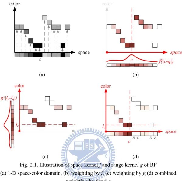
Fig. 2.1. Illustration of space kernel f and range kernel g of BF

(a) 1-D space-color domain, (b) weighting by f, (c) weighting by g,(d) combined weighting by f and g

Fig. 2.1 shows how kernel function f and g influent the weighting value for support pixel q. In Fig. 2.1 (a), for ease of show, we take one-dimension (1-D) image as spatial domain on x-axis and project intensity domain R onto the y-axis. Fig. 2.1 (b) shows that Gaussian function with argument space distance |c-q| is a low-pass filter; it gives higher weight on near-c support pixels and lower weight on farther ones. It is intuitive that the farther q is away from target pixel c, the smaller its impact should place on the final result. On the other hand, similar weighting mechanism is placed on the intensity difference of c and q. Fig. 2.1 (c) shows that Gaussian function with argument |Ic-Iq| gives support pixel higher weight if its intensity is similar to Ic. This is

also intuitive to realistic situation: two nearby pixels with similar intensity are likely

belongs to the same object. To multiplying the two function’s effect as Fig. 2.1 (d) shows: the point A, B, C, D, and E are regarded as outliers with zero weighting. Especially notes that point B is an outlier regarded by kernel g though it is adjacent to

c. Similarly, point C is an outlier regarded by kernel f though its intensity is Ic. That is

to say, either q is far away from c or Iq is dissimilar to Ic, the impact of q will be

negligible.

(a)

(b) Fig. 2.2. Smoothing Results

(a) Gaussian filter, (b) Bilateral filter

Before Tomasi [1] et al. proposed BF, the most typical smoother was Gaussian filtering (GF) or other low pass filtering. The typical smoothers suffered from blur-effect because they only considered space kernel. Many algorithms have proposed to eliminate this effect. Tomasi added a range kernel into GF to be BF; this is a simple but effective method. Fig. 2.2 compares BF with GF to show that the range kernel is the key component for edge-preserving. In Fig. 2.2 (a), GF is used to remove the chessboard-like noise in the dark area of the left image. The right image is its

result. It is obvious that GF produces smooth result on the pixel far from the edge (the area around the green pixel), whereas it produces blur effect near the edge. This because GF is blind to entirely different colors across the edge; it still mixes all colors within its window though the window steps across the edge. Therefore, in the output result, it appears a blur area at the both sides of the edge. Fig. 2.2 (b) shows that BF doesn’t produce blur effect because its window doesn’t step on the both sides of the edge to mix entirely different colors. As shown by the red window, the window of BF is trimmed by the edge because the bright-side pixels, which have entirely different color from the center color, are regarded as outliers by its range kernel.

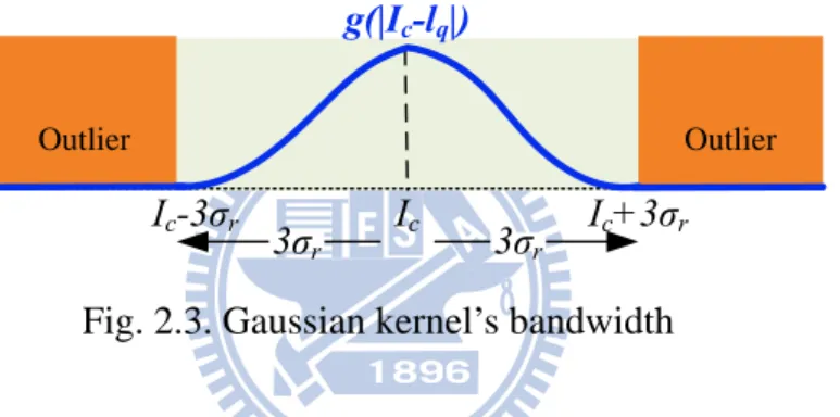
Ic Ic-3σr Ic+3σr 3σr 3σr Outlier Outlier g(|Ic-lq|)

Fig. 2.3. Gaussian kernel’s bandwidth

There is a parameter σr determining the degree of edge-preserving. It is defined by

the Gaussian function equation,

2 2 2 | | |) (| r q c I I q c I Ae I g σ − − = − , (2.2)

where A is a constant. As shown in Fig. 2.3, the Gaussian kernel’s bandwidth extends by about 3 times of σr. Outside the bandwidth, the value of g drops to below 0.01

which is negligible compare with the center weight. Any support pixel q with color outside the bandwidth will be regarded as the outlier. As a result, any edge with lager color differencewill be reserved (As last paragraph illustrates, this kind of edge trims kernel.). On the other hand, any edge with smaller color difference is blurred or smoothed as the noise.

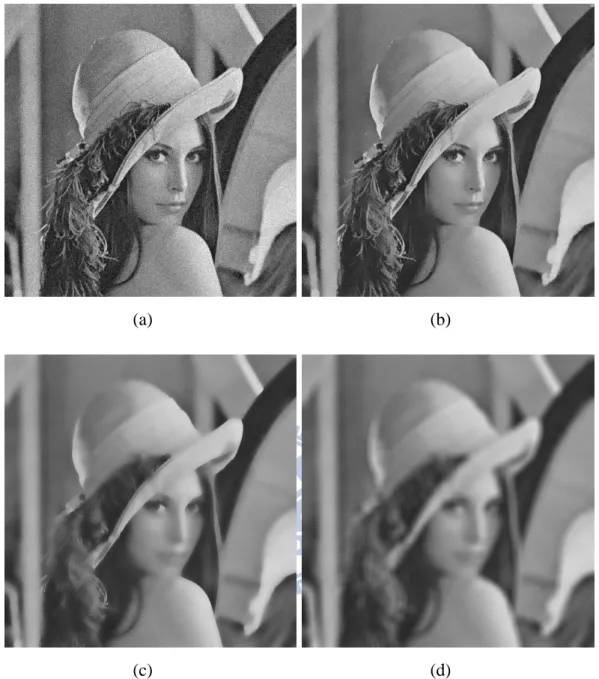
(a) (b)

(c) (d) Fig. 2.4. Smoothing results of BF with different range parameter σr

(a) noisy image, (b) σr=25, (c) σr=100, (d) σr= very large (GF).

Fig. 2.4 shows smoothing results of BF with different parameter σr choices. For, the

given noisy “Lina” shown by Fig. 2.4 (a), the value 25 is the best choice for σr to

separate noise and edges. If σr becomes larger as Fig. 2.4 (c), more edges are also

regarded as noise so that only the image structure is reserved. If σr is further set to a

very large value, BF will be simplified to GF because the color kernel becomes a constant function. As shown in Fig. 2.4 (d), the blur effect is obvious.

2.3. Application

We will recall applications of BF in this sub-chapter. They are mainly classified into de-noising, texture and illumination separation, and joint BF.

2.3.1. De-noising

De-noising or smoothing is the primary goal of BF. Other than being applied for 2-D image smoothing, it is also adapted for video processing and 3-D mesh smoothing. And many de-noise-related applications, such as flash and no-flash Image correction, are constantly proposed.

For video application, Bennett et al. [7] introduced BF into temporal smoothing. He assumes that the pixel variations in the temporal related same scene point over frames are affected by zero-mean noise. GF is used to reduce the noise level but it produces artifacts on moving object. Using BF instead can avoid these artifacts. For 3-D mesh smoothing, Jones et al. [8] and Fleishman et al. [9] simultaneously presented two similar approaches to adapt BF in the higher-dimension space. In the higher-dimension space, window computations for both kernels become more complex. Geometry properties such as mesh normal, projection, etc., are considered carefully.

On the other hand, in de-noise-related applications, Eisemann and Durand [10] used BF for flash and no-flash image correction. For a no-flash photo of a dark scene, although its illumination is correct, it has low signal-to-noise-ratio (SNR) that leads to inaccurate edge detection. However, a flash photo of the same scene has high SNR and higher discrimination of colors but it suffers from incorrect hard direct illumination. As shown in Fig. 2.5 [10], BF is used to smooth both photos for

de-noising and information extraction. BF helps departing their small-scale details and large-scale structure (This will be further discussed in 2.3.2). Finally, information from flash and no-flash photos is combined to form the final result without noise and with correct illumination and structure. Petschnigg et al. [11] also has proposed a similar correction algorithm based on this approach.

Fig. 2.5. Flow of flash and no-flash image correction [10]

2.3.2. Texture and illumination separation

Oh et al. [12] used BF as a separation algorithm to extract image texture and illumination component. They are motivated by the fact that in typical image, the illumination variation typically occurs at a large scale structure than small scale texture patterns; therefore, they proposed an approach using BF with suitable range kernel g to remove small-scale texture and preserve the large-scale illumination component. Simultaneously, the removed small-scale texture can also be extracted by

subtracting the large-scale component from origin image.

With the concept of above separation algorithm, Durand and Dorsey [13] isolated texture component from naïve intensity compression in tone mapping of high-dynamic range (HDR) image for low dynamic range display. This approach prevents the details in small scale texture being removed during compression. Other algorithms addressed in [14] and [15] also use the similar aspect.

2.3.3. Joint Bilateral Filtering

The BF used in the flash and no-flash image correction by Eisemann and Dorsey [10] is defined specially with the following equation,

(

)

(

)

(

)

(

)

∑

∑

∈ ∈ − − − − = S q c q S q c q q c I I g q c f J I I g q c f J JBF )( , (2.3)

where I is a guidance image, and J is another source image. Through the range kernel

g, the guidance image I could identify and suppress outliers for de-noising the source

image J. To emphasize that it joints guidance image influence into target source image, this specially defined BF is renamed as joint bilateral filtering (JBF).With this characteristic, JBF has been adopted in another flash and no-flash algorithm [15], image de-nosing [16] and disparity-map fusion [17],[18].

Further extending the applications of JBF, Kopf et al. [2] proposed the joint bilateral up-sampling that employed a high-resolution I to enlarge a low-resolution J for various image processing, such as tone mapping, colorization, disparity maps [19]-[21], demosaicing [22], texture synthesis [23]. A variety of JBF is the adaptive support weight (ADSW), a matching cost aggregation approach, proposed by Yoon and Kweon [3] for disparity estimation in 3D image processing. The disparity estimation is

based on matching corresponding pixels in different view frames. To increase matching correctness, disparity estimation uses filter-like convolution to aggregate support matching costs for target pixel. The ADSW employs the space and range kernels into aggregation to deliver better disparity maps than that produced by the traditional box filter. The concept of ADSW is further advanced in the disparity estimation algorithms of [24]-[28], and is also adopted by the developing MPEG standard, 3D Video Coding [5].

2.4. Summary

BF is an edge-preserving filter. Its parameter σr in range kernel can determine the

discontinuity in images to be either large-scale structure or small-scale texture (noise). The characteristic makes its application more than the primary goal of de-noising such as illumination and texture separation and JBF. Furthermore, with the guidance concept of JBF, BF applicable algorithms can be extended to various fields, such as disparity estimation for stereo process, up-sampling, and even the MPEG standard.

3. Related Work

Within BF applications, stereo processing is increasingly important in recent years. Many 3D-related entertainments, facilities, and industrials are pouring or on the horizon. Under this circumstance, BF and JBF must be ready for its potential real-time requirement of image and video processing. However, the big challenge for BF is its computational complexity in window computation. By brute-force implementation, BF takes extremely long running time on huge operations.

(a) (b)

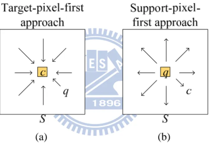
Fig. 3.1. Classification of acceleration approaches

Various acceleration approaches for BF have been proposed, and can be classified into two categories: target-pixel-first approach and support-pixel-first approach, according to their computational characteristics, as illustrated in Fig. 3.1. The target-pixel-first approach is an aggregation process that focuses on a target pixel c and accumulates its support pixels q. On the other hand, the support-pixel-first approach is a diffusion process that regards a support pixel q as a center to diffuse for its target pixels

c. With the classification, the milestone algorithms are listed in TABLE. 3-1.

The computational complexity and memory cost of the milestone algorithms are

also compared in TABLE. 3-1. Note that the former is shown by amount per pixel and the latter is shown by amount per frame. With this table, it is easy to approximate real amount of computations and memory cost of these algorithms for any size of target image. Take the brute-force implementation for example, referring to (2.1), for each pixel result, BF aggregates support pixels in the window S; therefore, the computational complexity is O(|S|2) which is associated to window size. This means if it processes an HD1080p image with a 31-pixel window width, the amount of required computations should be at the order of 2 billion (312x1920x1080). By software, the computationally expensive implementation takes minutes for a frame.

In the rest of chapter, we introduce the acceleration algorithms. In 3.1 and 3.2, support-pixel-first algorithms and target-pixel-first algorithms are introduced, respectively. Finally, in 3.3, we explain how we select algorithms from them for our proposed architecture design and implementation.

TABLE. 3-1 Comparison of computational complexity and memory cost in related work

Approach Computational Complexity

(per pixel)

Memory Cost (per frame)

Brute-Force All O(|S|2) 0

Support Pixel First

Basic LUT Construction O(|R|)

4MN 2-D Conv. by FFT O(|S|log|S|) Durand and Dorsey [13] Piecewise-linear Subsampling

LUT Construction O(|R|/sr) _4MN/s

s2

2-D Conv. by FFT O(|S|/ss2log(|S|/ss2))

Yang et al. [29]

Piecewise-linear LUT Construction O(|R|/sr)

4MN 2-D Conv. by Approx. Gaussian O(1) Paris and Durand [30]

Bilateral Grid LUT Construction O(|R|/sr) _MN|R|/(s

rss2)

3-D Conv. by FFT O(|S||R|/(srss2)log(|S||R|/(srss2)))

Target Pixel First

Pham and Vliet [31]

Separable 1-D Aggre. for Col. O(|S|) ₀

1-D Aggre. for Row O(|S|)

Basic Histogram Histogram Calculation O(|R||S|2) ₀

1-D Conv. O(|R|)

Huang [32]

Extended Histogram

Histogram Calculation O(|R||S|)

|S||R| 1-D Conv. O(|R|) Weiss [33] Distributed Histogram

Histogram Calculation O(|R|log|S|) _|S||E||R|

1-D Conv. O(|R|)

Porikli [34]

Integral Histogram

Histogram Calculation O(|R|/sr) _MN|R|/s

r

1-D Conv. O(|R|/sr)

M: frame height, N: frame width, |S|: window width, |R|: intensity range ss: quantization factor for S, sr: quantization factor for R, E: extension pixel count

3.1. Support-pixel-first Approach

Within support-pixel-first milestone algorithms, Durand and Dorsey’s piece-wise linear [13] is the first acceleration algorithm; Young’s algorithm [29] and Pairs’ algorithm [30] are partially related to it. Yong’s algorithm is boost of its constant time speed (independent of window width) and Paris’ algorithm proposes a brand-new spatial-intensity space.

3.1.1. Piece-wise linear algorithm and Yong’s algorithm

The range kernel makes BF nonlinear to spatial space; therefore, any spatial filter acceleration approach such as Fast Fourier Transform (FFT) doesn’t help to speed up BF. Instead of directly using the nonlinear equation of (2.1), Durand and Dorsey [13] approximate BF with a serial of frame-scale look-up tables (LUTs) defined as follows

(

)

(

)

(

)

(

)

(

)

(

)

∑

∑

∑

∑

∈ ∈ ∈ ∈ − − = − − − − = S q j q S q j q S q q S q q q c G q c f H q c f I j g q c f I I j g q c f j LUT )( , (3.1)

each of which associates to an intensity j that replaces the Ic of (2.1). The FFT can

accelerate the computation of (3.1) since both its numerator and its denominator become linear Gaussian convolution. The overall process includes two steps; at first, for every full-scale intensity j, its LUT is computed; that is, for a typical 8-bit image, 256 LUTs should be computed and stored. Second, for every pixel, its result is picked up from its intensity corresponded LUT by the following equation,

j I if j LUT I BF( )_c = ( )_c, _c = (3.2)

Besides, instead of using full-scale intensities, Durand and Dorsey [13] propose

piece-wise linear algorithm to reduce the number of LUT. With a quantization factor

sr, it only computes the LUT corresponds to intensity equals sr or its multiples. And

the result-picking function is rewritten as

⎪ ⎪ ⎩ ⎪ ⎪ ⎨ ⎧ < < − = − − − + − = j I s j if j I if s j LUT s s j I j LUT s I j j LUT I BF c r c c r r r c c r c c c , ) ( ) ( ) ( , ) ( ) ( . (3.3)

With (3.3), for the pixel without intensity corresponded LUT, its result is computed by bilinear interpolation of two LUTs of the most similar intensities.

Durand and Dorsey [13] further introduced a fast piecewise-linear algorithm with spatial space sub-sampling (quantization). The major computational complexity is O(|(S|/ss2)log(|S|/ss2)) per pixel in 2-D FFT, where ss is a spatial quantization factor.

The memory requirement is huge with cost 4MN/ss2 since at least four frame-scale

data, H j, G j, partial result of LUT(j) and previous result LUT(j-sr), are required under

the implementation of runtime updating LUT intensity by intensity [13].

Mostly based on piece-wise linear algorithm, Young et al. [29] used Deriche’s recursive method [35] to approximate Gaussian convolution of (3.1). They shows that this recursive method is able to run in constant time and the results are visually very similar to the exact. Therefore, the convolution process is reduced to O(1) complexity; and thus the major complexity of BF becomes O(|R|/sr) of LUT construction.

3.1.2. Bilateral grid

Paris and Durand [30] reformulated gray-level BF with a brand new 3-D space, bilateral grid. By their algorithm, it takes three steps to process BF; they are bilateral gird construction, 3-D Gaussian smoothing, and result extraction.

For bilateral grid construction, given a 2-D image, the first two dimensions of bilateral grid will correspond to the image spatial position (x,y) and the third dimension corresponds to the pixel intensity Ic. At the position (x,y,Ic), an non-zero

element is constructed. With all elements are constructed, in the second step, BF is computed by a 3-D defined Gaussian smoothing to associate weights w with intensities I and finally store each element with a vector (

∑

wI ,

∑

I). Because in bilateral grid the intensity is defined as an independent dimension, BF is linear for the 3-D Gaussian smoothing. Finally, in the result extraction step, the first two dimensions of bilateral gird correspond back to the position of 2-D image and set intensity there with the value,

∑

wI /

∑

I.

Paris and Durand further reduced the computational effort by down-sampling the three dimensions of bilateral grid with the spatial quantization factor ss for the first

two dimensions (spatial position) and the range quantization factor sr for the third

dimension (intensity). The computational complexity of the algorithm is

O([|S||R|/(srss2)][log(|S||R|/(srss2))]) of Gaussian smoothing. The memory cost is

MN|R|/(srss2) for storing the whole bilateral grid structure.

Following the bilateral grid scheme, Chen [36] further mapped this algorithm to GPU hardware, obtaining real-time processing for several megapixel images. In addition, Adams et al. [37] adopts the Gaussian KD-tree to improve its speed.

3.2. Target-pixel-first Approach

In TABLE. 3-1, the target-pixel-first algorithms can be mainly classified into two kinds of approaches: one is separable approach [31] and the other is histogram-based approach [32]-[34]. The separable approach uses two consequent 1-D BFs to speed up

the computation; Histogram-based approach uses range aggregation instead of spatial aggregation by histogram represented BF. Within its acceleration algorithms, integral histogram let the speed of BF implementation be independent of window width |S|.

3.2.1. Separable algorithm

Pham et al. [31] proposed this algorithm to approximate 2-D BF by two consequent 1-D BFs which computed by brute-force implementation: pixels within a row (column) are accumulated one by one and finally normalized. At first, by performing 1-D BF to all rows and their results make up a single column; and then, it performs 1-D BF again to the column for the final result. The computational complexity of separable algorithm is reduce to O(|S|) per pixel because 1-D window with length |S| is used for 1-D BF. Though it is significant faster than the brute-force implementation, the performance degrades linearly with window size. In addition, its axis-aligned 1-D BF makes it not suitable for the target image with complex patterns since its result suffers from the axis-aligned artifact.

3.2.2. Histogram & Huang’s algorithm

The histogram-based approach could reduce computation without significant quality degradation. The histogram representation of BF is defined as

(

)

(

)

(

)

(

)

(

)

(

)

∑

_∑

(

(

)

)

∑

∑

∑

∑

∑ ∑

∑ ∑

∑

∑

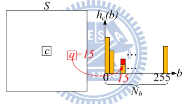
∈ ∈ ∈ = ∈ = ∈ = ∈ = ∈ ∈ − − = − − = − − = − − = R b c c R b c c R b c I b R b c I b R b I b c R b I b c S q c q S q c q q c b h b I g b b h b I g b I g b b I g b I g b b I g I I g I I I g I BF q q q q ) ( ) ( ] 1 [ ] 1 [ ] [ ] [ ) ( (3.4) 17

where hc is the pixel count histogram of the window S centered by c as illustrated in Fig.

3.2. The key point of these approaches is to convert its convolution from the space domain S to the range domain R, as shown in the summation index of (3.4). Thus, its computation includes two parts: histogram calculation and 1-D convolution. In the histogram calculation for hc, each support pixel q in S is classified by its intensity and

accumulated into its corresponding bin b. In other words, hc(b) refers to the number of

support pixels with the intensity b in S. Note that the number of bin Nb is 256 for the

exact result of typical 8-bit gray-level. In the 1-D convolution, (3.4) can be calculated with the given hc. For the basic histogram-based approach, the major computational

complexity is O(|R||S|2) in the histogram calculation.

Fig. 3.2. Concept of histogram-based approaches

Fig. 3.3. Concept of Huang’s algorithm

To speed up the histogram calculation, an early proposed Huang’s algorithm [32] can be applied. As shown in Fig. 3.3, windows of two consequently-processed pixels c and c’ are almost overlapped each other; therefore, the window histogram hc’ can be

updated from the processed window hc by two row histograms. The computational

complexity associates to the row histogram is O(|R||S|) which is significantly faster than the basic histogram approach if |S| is large. However, it spends extra memory cost with size |S||R| to store row histograms on overlapped region.

3.2.3. Weiss’ Distributed Histogram

Based on Huang’s algorithm, Weiss [33] proposed a distributed histogram approach that reassembles the histogram calculation of each row. The approach not only reuses histograms in vertically process direction, but it also reuses data horizontally during processing many column pixels together. Fig. 3.4 (a) illustrates an example of 5-column-parallel process during which Weiss algorithm keeps nine distributed histograms: he , which associates to the window of pixel e, and column

histograms h1-h8. Window histograms associate to targets c, d, f, g are computed from

these nine histograms as shown by Fig. 3.4 (b). In horizontal, the approach can be extended for more parallel columns with different set of distributed histograms. On the other hand, in vertical, these distributed histograms update by Huang’s algorithm.

Based on distributed histogram approach, Weiss further introduced hierarchical approach. Fig. 3.5 [33] shows an example of hierarchical distributed histogram which has yellow, orange, and red, totally three coarse-to-fine tiers. This hierarchical approach can reduce computational complexity to near O(|R|log|S|). For the memory cost, the approach uses Huang’s algorithm so that it also needs memory to store histograms. Furthermore, since histograms are distributed, the memory cost grows larger to |S||E||R|, where E associates to how many distributed histograms are used in parallel.

(a) (b) Fig. 3.4. Concept of Weiss distributed Histogram:

(a) distributed histograms, (b) computations of target histograms

Fig. 3.5. Three-tier hierarchical distributed Histogram [33]

3.2.4. Integral Histogram

(a) (b) (c)

Fig. 3.6. Concept of integral histogram

(a) Integral origin O and integral region (IR), (b) integration process, (c) an integral histogram of pixel X of the IH space

Porikli et al. [34] proposed this algorithm to make the computational complexity of histogram calculation independent of window size. The construction of integral histogram (IH) is like a space transformation process from a 2-D image space to a 2-D IH space. Prior to processing the transformation, we have to decide an integral origin

O and an integral region (IR) as illustrated in Fig. 3.6 (a). Fig. 3.6 (b) shows that

during the transformation with raster scan process from O to the end of IR, each pixel of 2-D IH space is given an IH. Fig. 3.6 (c) illustrates that the given IH at any pixel X is actually a quantized histogram (with quantized factor sr) for a 2-D image space

region stretches from O to X. Porikli et al. showed that quantized histogram doesn’t suffer from severe quality degrading for BF result; therefore, the number of histogram bins can be less than the number of intensity levels. In overall, the integration process’ computational complexity is O(|R|/sr) of pure histogram operations. And other details

will be further discussed in Chapter 4.1.

In IH space, arbitrary window histogram (as long as the whole window is within the IR) is computed from linearly combination of its four corner integral histograms ;therefore, the computational complexity is reduced to O(|R|/sr) that is

independent of window width |S|. The integral histogram approach can be faster than the brute-force approach when |R|/sr is smaller than |S|2. That implies this approach is

suitable to be applied when BF has large window size. In term of computational complexity, this algorithm is the state-of-art of the target-pixel first approach. But its memory cost is large with amount MN|R|/sr because of the frame-scale-magnitude

process, where MN is the area of the image. Other details of the extraction process are also discussed in Chapter 4.1.

3.3. Summary

In comparison, the support-pixel-first algorithms are iterative processed by frames and the target-pixel-first algorithms are progressive processed pixel-by-pixel in raster scan. For computational complexity, Young’s algorithm of the former and Porikli’s algorithm of the latter achieve constant time of O(|R|/sr). They both suffer from high

memory cost because of frame-scale-magnitude LUTs and histogram storage, respectively. In terms of implementation, the support-pixel-first approach is more suitable for multi-color-channel computing since they are defined by a multi-dimensional space. For the realization of gray level process, the support-pixel-first has achieved real time in GPU hardware and target-pixel-first approach is implemented by software program. However, we still choose target-pixel-first approach because its memory cost is likely to be reduced and other details are discussed in the next chapter.

4. Analysis of Integral histogram based JBF

The support-pixel-first approach can achieve real time process with GPU hardware. As mentioned before, GPU implementation is a general-purpose hardware. Although it may be implemented in embedded or source-restricted system, it still cost expensive. For a specified low cost implementation, VLSI implementation may be a more proper candidate. In addition, both support-pixel-first and target-pixel-first approaches suffer from high memory cost; however, the cost of the latter is likely to be reduced by taking advantage of its progressive process, whereas the cost of the former must be frame-scale-magnitude because of its iterative process by frames. Therefore, in the thesis, we focus on VLSI implementation of target-pixel-first approach for BF or JBF. Within its algorithms, integral histogram is the state-of-art.

To combine integral histogram and JBF, Ju and Kang [38] modified (3.4) to

(

)

(

)

(

)

(

)

(

)

(

)

_∑

∑

(

(

)

)

∑

∑

∑

∑

∑ ∑

∑ ∑

∑

∑

∈ ∈ ∈ = ∈ = ∈ = ∈ = ∈ ∈ − ′ − = − − = − − = − − = R b c c R b c c R b c I b R b c I b q R b I b c R b I b c q S q c q S q c q q c b h b I g b h b I g b I g J b I g b I g J b I g I I g J I I g J JBF q q q q ) ( ) ( ] 1 [ ] [ ] [ ] [ ) ( . (4.1)

Different from (3.4), the histogram in the numerator is the pixel intensity histogram h’c

that accumulates the pixel intensity for each bin, instead of the pixel count in hc. In this

chapter, we introduce the integral histogram approach in details, and then analyze the design challenges of integral-histogram-based JBF, which can also be applied to BF.

4.1. Integral histogram based JBF

TABLE. 4-1 Computational flow and complexity analysis for each pixel in the integral histogram based JBF

Process Complexity (operation) BW for IH (data) BW for pixel (data) Integration process:

Pixel count histogram hc

Loop b=0 to Nb-1

IHOS(b)=IHOQ(b)+IHOR(b)-IHOP(b)

IHOS(IS) += 1

Pixel Intensity histogram h’c

Loop b=0 to Nb-1

IHOS(b)=IHOQ(b)+IHOR(b)-IHOP(b)

IHOS(IS) += Js ADD: 3Nb ADD: 1 ADD: 3Nb ADD: 1 4Nb 4Nb 2 pixels Extraction process:

Pixel count histogram hc

Loop b=0 to Nb-1

hc(b)=IHOD(b)+IHOA(b)-IHOB(b)-IHOC(b)

Pixel Intensity histogram h’c

Loop b=0 to Nb-1

hc(b)=IHOD(b)+IHOA(b)-IHOB(b)-HOC(b)

ADD: 3Nb

ADD: 3Nb

4Nb

4Nb

Kernel calculation process: Loop b=0 to Nb-1 G(b) = g(|Ic-b|) ADD, LUT: Nb 1 pixel Convolution process: Nu=0, De=0 Loop b=0 to Nb-1 De += G(b) x hc(b) Nu += G(b) x h’c(b) Result = Nu / De MUL, ADD: Nb MUL, ADD: Nb DIV: 1 1 pixel Total 17Nb+3 16Nb 4 pixels

TABLE. 4-1 presents the computational flow and computational analysis of the integral histogram based JBF to calculate 1-pixel result, which consists of the

integration, extraction, kernel calculation, and convolution processes. In which, the

former two are for the histogram calculation step, and the latter two are for the 1-D convolution step. Especially note that these processes, for each pixel, should compute for all bins of related histograms; therefore, their complexity and bandwidth for integral histogram (bandwidth for IH) are the multiple of the number of bin, Nb.

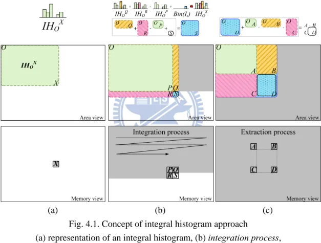
For ease of explanation, we use the area view (image space) to show how this

approach operates and the memory view (IH space) to show the memory usage, as illustrated in Fig. 4.1 (a). In the area view, IHOX is a histogram of the rectangular area

stretched from the pixel O to X. Thus, the addition and subtraction of IH can be regarded as area merging and cutting, respectively. In the memory view, the data of

IHOX are stored at X, and the gray region represents occupied memory usage. With these

representations, Fig. 4.1 (b) and (c) illustrate the integration and extraction processes.

(a) (b) (c) IHOQ IHOR IHOP Bin(Is) IHOS + - + O P O R O _Q O S S

Fig. 4.1. Concept of integral histogram approach

(a) representation of an integral histogram, (b) integration process, (c) extraction process.

First, the integration process progressively calculates the IH of each pixel using the equation, ) ( _S P O R O Q O S O IH IH IH Bin I IH = + − + (4.2)

For the pixel count histogram hc and the pixel intensity histogram h’c, their IHs are

computed separately as shown in TABLE. 4-1. The histogram IHOS is computed from

linearly combination of three exist integral histograms and a histogram of the target pixel IS. We show the target pixel histogram with the notation Bin(IS) because the

histogram must be a one-hot histogram. For hc, Bin(IS) is 1 for the corresponding bin

and 0 for others; on the other hand, for h’c, this term is Js for the corresponding bin, and

also 0 for others. Adding the one-hot histogram updates only the bin corresponding to

IS so that, as shown in TABLE. 4-1, it is perform outside the loop. After this process,

the IH of each pixel is produced and stored into memory.

Second, given the IHs, the extraction process can extract hc or h’c, the histograms of

the window ABCD, which is centered by the target pixel c, is defined by equation, C O B O A O D O ABCD c corh H IH IH IH IH h ' = = + − − (4.3)

As shown in Fig. 4.1 (c), a histogram with arbitrary window size can be obtained by using the IHs of four corners. With this property, the integral histogram approach can reduce computational complexity to O(|R|/sr) which is independent of window size.

Third, the kernel calculation process computes the range kernel by a range table, which includes 256 items for the 256 possible values of |Ic-b|. Finally, given the range

kernel g and the histograms hc and h’c, the convolution process calculates the result of

target pixel c by (4.1).

4.2. Design Challenge

Since the complexities listed in TABLE. 4-1 are pixel wise as well as bin number dependent, they will grow quickly, as shown in Fig. 4.2, as resolution and bin number grow. The detailed design challenges are described below.

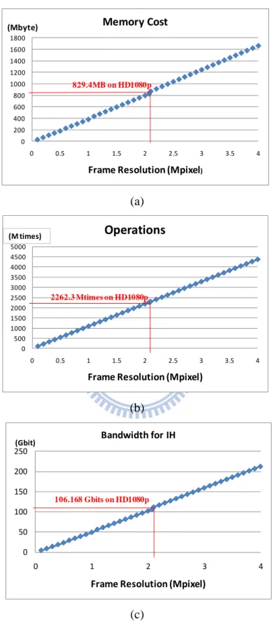
0 200 400 600 800 1000 1200 1400 1600 1800 0 0.5 1 1.5 2 2.5 3 3.5 4 Frame Resolution (Mpixel) Memory Cost (Mbyte) 829.4MB on HD1080p (a) (b) 0 500 1000 1500 2000 2500 3000 3500 4000 4500 5000 0 0.5 1 1.5 2 2.5 3 3.5 4 Frame Resolution (Mpixel) Operations (M times) 2262.3 Mtimes on HD1080p 0 50 100 150 200 250 0 1 2 3 4 Frame Resolution (Mpixel) Bandwidth for IH (Gbit) 106.168 Gbits on HD1080p (c)

Fig. 4.2. Analysis of Design Challenges over frame resolutions With Nb=64; (a) Memory cost, (b) Operations, (c) Bandwidth for IH

4.2.1. High Memory Cost for integral histograms

During the integration process, all the IHs of whole image are stored in memory. BF needs a frame-scale-magnitude memory for hc, and JBF additionally needs another

one for h’c. Therefore, the total memory cost of JBF is

) 8 ( + ⋅ + ⋅N_bw_b MN N_b w_b MN (4.4)

where the former term is for hc, and the later term is for h’c. M and N is the frame height

and width, Nb is the number of bin, and wb is the bit width of a bin. Note that wb is

related to the maximal integral area, and its value equals log2(MN). In addition, the bit

width of h’c is more than hc by 8 bits because pixel intensity is 8 bits.

Above memory cost would be 829.4 Mbytes for the HD1080p resolution as listed in Fig. 4.2 (a) and TABLE. 6-4. For a VLSI design, these massive data could be configured into off-chip memory (i.e. DRAM) or on-chip memory (i.e. SRAM). However, compared to the on-chip memory, the off-chip memory suffers from longer access latency due to its complicated controlling mechanism [39], and limited bandwidth usage due to bus sharing by multiple masters. Hence, our strategy for the high memory cost is to reduce the memory requirement and enable data to be stored in on-chip memory for fast implementation.

4.2.2. High Computational Complexity in All Processes

According to the complexity in TABLE. 4-1, generating 1-pixel result needs 15Nb+2 additions, 2Nb multiplications, and 1 division. If Nb is 64, the total complexity

will be 2,262.3 million operations for an HD1080p image as shown in Fig. 4.2 (b). To meet above demands, a VLSI design with sufficient parallel operators is necessary.

4.2.3. High Bandwidth in Integration and Extraction

In TABLE. 4-1, the bandwidth for IH requires 16Nb for 1-pixel result, and that will

reach 106.168 Gbits for an HD1080p image as shown in Fig. 4.2 (c) and TABLE. 6-4. That is because the IHs are accessed frequently. With the strategy for the memory cost problem, the IHs are stored in on-chip memory, and its data bus should be increased to address the high bandwidth problem. However, it results in over-partitioned memory and increased area. Thus, a method which can reduce the bandwidth is needed.

4.2.4. Large Range Table in Kernel Calculation

In the kernel calculation process, a range table with 256 items is needed. However, with the parallel operations for the computational complexity problem, this table should be duplicated. By straightforward implementation, 256 range tables, each of which corresponds to 256 possible values of (Ic - Iq), must be available for parallel

operations. Both the size (number of items) and the number of the range table result in large area; therefore, a table-reduction method and a table-reuse method are needed

4.3. Summary

In conclusion, for example of the HD1080p image, the integral histogram approach needs the memory cost of 829 Mbytes and the bandwidth of 106 Gbits per frame. In addition, the Porikli’s approach still suffers from high computational complexity of 2,262 million operations even though it has been accelerated by integral histogram approach. Moreover, the 1-D convolution needs a large range table with 256 items for the range kernel. Due to above problems, it is hard to achieve a real time performance

and thus demands VLSI hardware acceleration. In the next chapter, we will introduce our proposed memory reduction methods. And then in Chapter 6, a VLSI implementation with problem solving architecture will be addressed.

5. Proposed Memory Reduction Methods

5.1. Overview

To solve the high memory cost problem mentioned in last chapter, we propose three memory reduction methods. First, the runtime updating method (RUM) takes advantage of progressive raster-scan process to discard unnecessary data. Second, the stripe based method (SBM) avoids frame wide memory cost by dividing each frame into vertical stripes and processing them one by one. Finally, the sliding origin method (SOM) lessens the storage data dependency of the original histogram integration process to reduce the memory requirement from frame-scale-magnitude to line-scale-magnitude. With these memory methods, the memory cost can be reduced to 0.003%-0.020%. The details of the proposed methods are described below.

5.2. Runtime Updating Method (RUM)

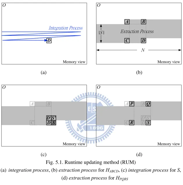
The concept of the RUM is to perform the integration process and the extraction

process at the same time, instead of two separate iterations in the original flow. Fig. 5.1

illustrates its memory configuration in the memory view. In Fig. 5.1 (a), the integration

process is performed from the integral origin O to D. In the meanwhile, the extraction process can extract the histogram HABCD as shown by Fig. 5.1 (b). From the data

lifetime analysis for raster-scan, this is the last time taking IHOA into extraction

process. And all the IHs before the pixel A will not be used for extraction process anymore. Hence, only the IHs from the pixel from A to D require memory space. Thus, the memory cost is

) 8 ( | | | |S N⋅N_bw_b+ S N⋅N_b w_b+ (5.1)

where M in (4.4) is replaced by the window width |S|.

D O Memory view D B A C | | O Memory view (a) (b) D B A C D'S'S O D B A C D'S'S O P Q R

Memory view Memory view

(c) (d)

Fig. 5.1. Runtime updating method (RUM)

(a) integration process, (b) extraction process for HABCD, (c) integration process for S,

(d) extraction process for HPQRS

Fig. 5.1 (c) and (d) illustrate the memory updating process when the two processes moves right to the next pixel S. In Fig. 5.1 (c), the integration process calculates the new IHOS using IHOD, IHOD’, IHOS’, and then the new IHOS can overwrite the memory

position of the discarded IHOA. In Fig. 5.1 (d), the extraction process extracts HPQRS. On

the whole, in raster scan from integral origin O to the end of region, the proposed RUM alternates between these two processes repeatedly.

With the proposed RUM, the memory cost could be reduced from a full frame to a partial frame. This method can gain considerable reduction since |S| is usually much smaller than M.

5.3. Stripe Based Method (SBM)

(a) (b)

Fig. 5.2. Stripe based method (SBM)

(a) partitioned-frame, (b) extended integral region for each stripe

(a) (b)

Fig. 5.3. Integral region of SBM is an extended stripe. (a) four corner IHs for extraction process, (b) integration process.

The main idea of the SBM is to slice the whole frame into many vertical stripes, and

the integration and extraction processes are performed stripe by stripe. Fig. 5.2 (a) illustrates a frame partitioned into stripes, and Fig. 5.2 (b) illustrates the extended region for a stripe.

Fig. 5.3 (a) shows that, in the extraction process, some corner IHs, such as A and B, are outside the stripe. Therefore, as shown in Fig. 5.3 (b), the integration process should be carried out at extended region to make sure these outside-stripe IHs are defined. On both stripe boundaries, the integral region (IR) is extended by half the window width, |S|/2, to include the regions that can be traversed by window corners. Note that these IHs are associated with new origin O’ instead of O.

As shown by Fig. 5.2 (b), the IR of each stripe is (|S| + ws -1) pixels wide.

Compare with the original, the IR is reduced from a frame to an extended stripe; as a result, the bit width wb can be smaller.The total memory cost of the SBM is

(

|S|+w_s −1

)

⋅N_bw_b +M

(

|S|+w_s −1

)

⋅N_b(w_b +8)

M , (5.2)

where ws is the stripe width, and wb equals log2[M(|S|+ws-1)]. Compared to the original

cost of (4.4), the SBM could significantly reduce memory if the stripe width, (|S|+ws-1), is much smaller than N.

Fig. 5.4. Overlapped integration region between two adjacent stripes

The overhead of the SBM is that the extended regions result in extra computation

and bandwidth due to repeatedly performed integration processes on these regions as shown by Fig. 5.4. Thinner stripes can reduce memory cost more, but that leads to more overheads. Thus, the selection of ws is a tradeoff between memory reduction and

overheads. That will be discussed in Chapter 6.6.

5.4. Sliding Origin Method (SOM)

(a) (b)

(c)

(d)

Fig. 5.5. Sliding Origin Method (SOM)

(a) Sliding origin O, (b) extraction process with sliding origin O, (c) integration process for next pixel S, (d) modified integration process

The concept of the SOM is to vertically slide the origin pixel O with the integration and extraction processes to reduce memory cost from a plane to a single line. As shown in Fig. 5.5 (a), the origin pixel O slides downward to keep pace with the top row of the window ABCD. With the SOM, the integration and extraction processes can be simplified as described below.

Fig. 5.5 (b) shows that, for the extraction process, the original IHOA and IHOB cannot

form meaningful histogram rectangles in area view because the position of O is under

A and B. Hence, these two histograms are zero and (4.3) can be simplified as the

following equation, C O D O C O B O A O D O ABCD IH IH IH IH IH IH H − = − − + = (5.3)

Fig. 5.5 (c) shows that, for the integration process, the new IHOS is computed by

) ( _S D O S O D O S O IH IH IH Bin I IH = + ′− ′ + _(5.4)

However, the S’ and D’ are on the previous row, and by SOM they should have been defined by the previous origin O’ as shown in Fig. 5.5 (d), instead of O. Therefore, for real process, the IHOS’ and IHOD’ in (5.4) should be changed to IHO’S’ and IHO’D’ by the

following derivation, which is corresponding to the area view of Fig. 5.5 (d).

(

) (

)

(

)

(

) (

) ( ) ( ) ( ) ( ) ( ) ( S D O Q S O D O S B O D O Q B O S O D O S B O D O Q O S O D O S D O S O D O S O I Bin IH I Bin IH IH I Bin IH IH I Bin IH IH IH I Bin IH IH IH IH IH I Bin IH IH IH IH + − − + = + − − + − + = + − − − + = + − + = ′ ′ ′ ′ ′ ′ ′ ′ ′ ′ ′ ′ ′ ′ ′ ′ ′ ′

)

(5.5)

Compare with (5.4), final line of (5.5) shows that only a slight change is required (it adds the term of subtracting Bin(IQ)) for the integration process to let the integral

origin slide from O’ to O.

However, the slight change makes significant difference on the memory cost. With above simplification, only the IHs of C, D, S’ and D’ are associated, and by the concept of RUM, only a single row of IHs from D’ to D, requires memory space as shown in Fig. 5.6 (a). Thus, the total memory cost is reduced as

) 8 ( + ⋅ + ⋅N_bw_b N N_b w_b N (5.6)

where wb equals log2(|S|N) since the maximal IR is |S|N as shown by Fig. 5.6(b).

Compared to the original cost of (4.4), the height dimension M is replaced by |S|, and

wb is much smaller because |S| is usually much smaller than image width M.

(a) (b)

Fig. 5.6. Sliding Origin Method

(a) Memory Cost, (b) Maxima integral region.

5.5. Combination

(a) (b)

Fig. 5.7. Combination of memory reduction methods (a) Memory Cost, (b) Maximum integral region

The proposed memory reduction methods could be easily combined as shown by Fig. 5.7 (a). First, the SBM partitions a whole frame into stripes. Then, by stripes, the RUM and SOM are performed row by row. This combination can reduce the memory cost to

(

|S|+w_s −1

)

⋅N_bw_b +

(

|S|+w_s −1

)

⋅N_b(w_b +8) (5.7) where wb equals log2[|S|(|S|+ws-1)], |S|(|S|+ws-1) is the area of maximum integral

region as shown by Fig. 5.7 (b). Compared to the original cost of (4.4), M is decreased to 1 since the SOM reduces data dependency of the extraction process and the RUM discards unnecessary data. Besides, N is decreased to (|S|+ws-1) since SBM cuts image

into narrow stripes. Note that in this memory cost formulation, Nb and |S| are related to

the application quality, and ws is related to hardware performance. The analysis of

parameter selection will be further presented in Chapter 6.6.