採用模糊資訊的推理：方法與應用

全文

(1)國立交通大學資訊管理研究所博士論文. 採用模糊資訊的推理：方法與應用 Reasoning with Fuzzy Information: Methods and Applications. 研究生：高韓英指導教授：黎漢林博士. 中華民國九十三年六月.

(2) 採用模糊資訊的推理：方法與應用 Reasoning with Fuzzy Information: Methods and Applications. 研究生：高. 韓. 英. Student：Han-Ying Kao. 指導教授：黎. 漢. 林. Advisor：Han-Lin Li. 國立交通大學資訊管理研究所博士論文. A Dissertation Submitted to Institute of Information Management College of Management National Chiao Tung University in Partial Fulfillment of the Requirements for the Degree of Doctor of Philosophy in Information Management June 2004 Hsinchu, Taiwan, Republic of China. 中華民國九十三年六月.

(3) Dedication. To Dad, Mom, Leo and Athena, who complete me..

(4) 採用模糊資訊的推理：方法與應用學生：高韓英. 指導教授：黎漢林國立交通大學資訊管理研究所博士班. 摘. 要. 對於專家系統或是決策支援系統而言，推理是一項重要的工作。現實世界中，有三類常見的推理工作：預測、診斷、與規劃。在形形色色的知識庫與運算機制中，貝氏網路與影響圖是很普遍的圖形化模式，常用來處理不確定情況下的推理與決策。過去有許多學者提出各種演算法，試圖解決貝氏網路或影響圖上的查詢。然而，這些方法通常存在一些限制。首先，相關的參數或機率值，必須是確定而非模糊的。當決策或推理環境中，無法取得確定的知識，而只能取得不完整或是模糊的資訊時，推理工作將難以進行。其次，傳統貝氏網路的推理方法，難以考慮額外的限制。再者，不同的推理工作無法同時完成，例如診斷與決策之規劃。鑑於上述之限制，本論文擴展傳統的貝氏網路，而發展出一般性的貝氏網路，在這一般性的貝氏網路中，有幾個重要的組成集合：離散隨機節點之集合、連續隨機節點之集合、決策節點之集合，確定性參數之集合、與模糊參數之集合。除了傳統上只考慮離散隨機節點與確定參數的推理演算法，本論文研究三類貝氏網路的特殊題型，並提出解答的方法。這三類特殊推理題型為：(1) 考慮離散隨機節點與模糊參數之診斷，(2) 考慮離散隨機節點與模糊參數之診斷及決策，與(3) 考慮連續隨機節點之診斷與決策。本論文的特色包含下列幾點：(1) 擴展傳統的貝氏網路，而發展出一般性的貝氏網路，其中考慮：離散隨機節點之集合、連續隨機節點之集合、決策節點之集合，確定性參數之集合、與模糊參數之集合。此一般性的貝氏網路，將作為本研究的基礎架構。 (2) 解決在一般性貝氏網路上的模糊推理問題，包括牽涉模糊參數與可能性分配的題型。 (3) 在推理的過程中，考慮無法納入正規知識庫的額外的限制或知識。(4) 在靜態與動態的環境下，解答針對貝氏網路的查詢。(5) 將發展的推理模式與方法，應用於醫療資訊或供應鏈管理的個案。所有的應用個案皆有詳細的解說。關鍵詞: 模糊推理，貝氏網路，影響圖，供應鏈管理，醫療資訊。. i.

(5) Reasoning with Fuzzy Information: Methods and Applications Student：Han-Ying Kao. Advisor：Han-Lin Li Institute of Information Management National Chiao Tung University. ABSTRACT Reasoning is a major task to an expert system or a decision support system. Three types of reasoning tasks prevail in real-world applications: prediction, diagnosis and planning. Among the various knowledge bases and computation schema, Bayesian networks and influence diagrams are well-known graphical models for reasoning and decision-making under uncertainty. Many algorithms have been designed to answer the queries on a Bayesian network or an influence diagram. However, several limitations persist in the conventional methods. First, all relevant parameters are assumed to be crisp. Second, extra constraints or knowledge regarding belief propagation in Bayesian networks are difficult to embed. Third, diagnosis and planning cannot be completed in the same place. Motivated by the limitations mentioned above, this dissertation extend the traditional Bayesian networks to general Bayesian networks (GBN) that are composed of several components: the set of discrete random nodes, continuous random nodes, decision nodes, crisp parameters, and fuzzy parameters. In addition to the conventional reasoning problems that consider only crisp nodes and crisp parameters, three categories of reasoning are solved as the special cases (subsets) of general Bayesian networks: (1) diagnosis with discrete random nodes and fuzzy parameters; (2) diagnosis and decision-making with discrete random nodes and fuzzy parameters; and (3) diagnosis and decision-making with continuous random nodes in dynamic environments. The distinguished features of this dissertation include: (1) extend the traditional Bayesian networks to general Bayesian networks, including discrete random nodes, continuous random nodes, decision nodes, crisp parameters, and fuzzy parameters. The general Bayesian networks are induced as the general research framework; (2) solve fuzzy reasoning tasks in three subsets of GBN where fuzzy parameters and possibility distributions are considered; (3) consider extra knowledge or constraints for the belief propagation, which are not implemented in the formal knowledge bases; (4) answer the queries from Bayesian networks in dynamic as well as static environments; (5) the reasoning models and methods are applied to the cases from medical informatics and supply chain management. All the applications are developed and illustrated in details. Keywords: fuzzy reasoning, Bayesian networks, influence diagrams, supply chain management, medical informatics. ii.

(6) 誌. 謝. 能夠完成這本論文，將博士班學業告一段落，心中充滿無限的感恩。首先，我想謝謝指導教授黎漢林老師，六年來對我的耐心教誨與指引，包容我這個平庸的學生，讓我有機會練習獨立研究，並且學著認真呵護、珍愛自己的每一篇作品。黎老師對研究的執著、與帶領學生的苦心，亦是我想努力學習的。若我在博士班期間，有任何學術上的成果，都要歸功於黎老師。計畫書及論文口試期間，對於口試委員王小璠教授、游伯龍老師、曾國雄老師、陳茂生教授、溫于平教授的指正，感到完全地折服與受用。這段時間的收穫，比我預期的超出許多，也見識到老師們嚴謹治學、提攜後進的熱誠。您們將是我在日後學術生涯中，效法與趨近的目標。一起用功的同學～菁蓉、念祖、榮發、嘉珍等，還有好多同研究室的學弟妹們，謝謝你們，讓我在交大得有歸屬感、學習的路上從不寂寞。家人的支持與鼓勵，是我堅實的後盾。先生嘉輝總是陪在我身邊，分享我的笑聲與淚水，給我安全停泊的港口；博三時女兒悅珊的出生，為我們的生活帶來無比的歡愉，也讓我對女性的堅韌潛力，產生充分信心。最感謝的，是一直無條件欣賞我的爸爸高智雄先生、與媽媽劉純美女士～不管人生境遇如何，總是那麼愛我、相信我；還有我最可愛的親手足～姊姊岱伶、妹妹巧巧與岱琪、弟弟韓中，讓我在人生的歷程中，常有知音的陪伴。最後，我想將博士學位的榮耀，獻給天國的兩位女性～我的祖母陳月琴女士 (1914~1992) 與駱月裡女士(1915~1998)。她們的智慧、美麗、與慈愛，遠非我所能及，但卻選擇在上個世紀，將她們的一生奉獻給家庭。是她們讓我瞭解到女性的胸襟與偉大，教我懂得珍惜現代女性所掌握的幸福，也促使我更堅定這一生所追求的目標。口試結束，當老師們向我恭賀時，我並沒有預期的狂喜，有的只是學而無涯的自省，與任重而道遠的自我鞭策。我會繼續努力的。. iii.

(7) Contents 摘要. .........................................................................................................................i. Abstract. ........................................................................................................................ii. 誌謝. .......................................................................................................................iii. Contents. .......................................................................................................................iv. Tables. .......................................................................................................................vi. Figures. ......................................................................................................................vii. Chapter 1. Introduction ....................................................................................................1. 1.1. Research background......................................................................................1. 1.2. Research Objectives and Framework .............................................................4. Chapter 2. Literatures review .........................................................................................10. 2.1. Expert systems and probabilistic reasoning .................................................10. 2.2. Bayesian networks........................................................................................12. 2.3. Fuzzy sets and theory ...................................................................................14. Chapter 3. Diagnosis with fuzzy parameters..................................................................16. 3.1. Reasoning with crisp information ................................................................16. 3.2. Problem and goals ........................................................................................21. 3.3. Model development ......................................................................................24 3.3.1. Fuzzy parameters..............................................................................24. 3.3.2. Fuzzy Abductive Models ..................................................................26. 3.4. Solution and illustrative examples................................................................28. 3.5. Discussions and conclusions ........................................................................37. Chapter 4. Diagnosis and decision with fuzzy parameters.............................................39. 4.1. Influence diagrams .......................................................................................40. 4.2. Problem and goals ........................................................................................47 iv.

(8) 4.3. Model development ......................................................................................49. 4.4. Algorithm and solutions ...............................................................................53. 4.5. Discussions and conclusions ........................................................................56. Chapter 5. Diagnosis and decision with fuzzy nodes.....................................................59. 5.1. Reasoning in supply chain management ......................................................59. 5.2. Problem and Goals .......................................................................................61 5.2.1. Dynamic Bayesian networks with fuzzy nodes................................64. 5.2.2. Uncertainties in supply chains..........................................................64. 5.3. Model development ......................................................................................65. 5.4. Algorithms and solutions..............................................................................74. 5.5 Chapter 6. 5.4.1. Phase I: diagnostic phase..................................................................74. 5.4.2. Phase II: Optimization phase............................................................78. 5.4.3. Linearization strategies.....................................................................87. Discussions and conclusions ........................................................................90 Discussions and conclusions ........................................................................93. 6.1. Discussions ...................................................................................................93. 6.2. Future extensions..........................................................................................95. 6.3. Concluding remarks......................................................................................96. References ......................................................................................................................98. v.

(9) Tables Table 1. The Associated Conditional Probability Distribution of Figure 1(b) ................7. Table 2. The membership functions of fuzzy probabilities ...........................................22. Table 3. Solution of Example 2.1. .................................................................................32. Table 4. The conditional probability distribution of Example 2.2. ...............................34. Table 5. The membership functions of fuzzy probabilities in Example 2.2..................35. Table 6. Solution of Example 2.2. .................................................................................38. Table 7. The conditional probabilities of pathogens, tests, and signs of UTI ...............44. Table 8. The conditional probabilities of Signs ( Signi )................................................45. Table 9. Conditional probabilities of Coverage with resistance ( Resist =1) ................45. Table 10. The membership functions of fuzzy probabilities ...........................................50. Table 11. Solution of Example 3 .....................................................................................58. Table 12. Description of nodes in the dynamic influence diagram in Figure 11.............69. Table 13. The probability/possibility distributions for the dynamic Influence Diagrams in Example 4....................................................................................................71. Table 14a The results of simulation ( λ -level = 0.0)........................................................79 Table 14b The results of simulation ( λ -level = 0.5)........................................................80 Table 14c The results of simulation ( λ -level = 1.0): ......................................................81 Table 15. Description of IT solutions ..............................................................................83. Table 16. Estimated costs/utilities of IT solutions in Example 4 (scale: 0 to 100) .........84. Table 17. The possibility functions of the fuzzy parameters in Example 4. ...................85. Table 18. Solution report of Example 4...........................................................................91. vi.

(10) Figures Figure 1. (a) an example of Bayesian networks, (b) the tree structure as clustering B and C into Z .............................................................................................6. Figure 2. Research framework of the dissertation ......................................................9. Figure 3. The membership function µ ~x1 ( x1 ) of ~ x1 ...................................................20. Figure 4. The membership function µ ~x7 ( x7 ) of ~ x7 .................................................20. Figure 5. A membership function of fuzzy probability.............................................24. Figure 6. A Bayesian network of the relationships between JITP techniques and performance measures ...............................................................................34. Figure 7. The input-output diagram of the optimization model for Chapter 4 .........42. Figure 8. A revised Bayesian network for Urinary tract infection............................43. Figure 9. Research framework of Chapter 5 .............................................................61. Figure 10. Cause-effect diagram of the two-echelon automotive supply chain..........63. Figure 11. A dynamic influence diagram of the supply chain ....................................67. Figure 11a Time expansion of the dynamic influence diagram in Figure 11 ..............68 Figure 12. A schematic view of DSS ..........................................................................96. vii.

(11) Chapter 1 Introduction Reasoning algorithms is a core issue to an expert system or a decision support system. In many domains, such as medical inference or industrial informatics, there are at least three types of reasoning tasks in a decision support system: prediction, diagnosis, and decision-making [32,41]. To conduct the reasoning tasks, an expert system or decision support system needs a knowledge representation mechanism for the knowledge base. Bayesian networks are commonly used graphical probabilistic models for the knowledge base. This chapter will review the basics of expert systems and reasoning.. 1.1. Research background Expert systems are a kind of information systems which should be able to process an. memorize information, learn and reason in both deterministic an uncertain situations, communicate with human and/or other expert systems, make appropriate decisions, and explains why these decision work. Castillo et al [2] classified the problems that an expert system can deal with into two types: deterministic and stochastic. Deterministic problems can be formulated using a set of rules that relates several well-defined objects. Experts systems that deal with deterministic problems are known as rule-based expert systems. In stochastic or uncertain situations it is necessary to introduce some means for handling uncertainty, such as certainty factors, fuzzy logic, probability, and so on. Expert systems that use probability as a measure of uncertainty are know as probabilistic expert systems, and the strategy they use is know as probabilistic reasoning or probabilistic inference. The ability to use both predictive and diagnostic information is an important component of plausible reasoning, and improper handling of such information leads to strange results. So, Pearl [35] classified the patterns of plausible 1.

(12) reasoning into abductive reasoning and inductive reasoning. Deduction, or prediction, is a logical process from a hypothesis to deduce evidence where probabilistic relationships are involved [35]. For example, if A is true, then B is true; that is A implies B. Abductive reasoning, or diagnosis, is a logical process that hypothetically explains experimental observations. For example, if A implies B, then finding B is true makes A more credible. This dissertation will focus on the abductive reasoning and decision-making models in expert systems. In this dissertation, Bayesian networks and influence diagrams play a central role in the uncertainty formalism. Bayesian networks [34,35] are directed acyclic graphs (DAG) in which the nodes represent the variables, the arcs represent the direct causal influences between the linked variables, and the strengths of these influences are expressed by forward conditional probabilities. The semantics of Bayesian networks demands a clear correspondence between the topology of a DAG and the dependency relationships portrayed by it. They are widely used knowledge representation and reasoning tools for various domains under uncertainty [1,2,4,8,13-18,20,23,27,34,35]. Influence diagrams are a special type of Bayesian networks with three kinds of nodes: decision nodes, chance nodes, and a value node. Decision nodes, shown as squares, represent choices available to the decision-makers. Chance nodes, shown as circles, represent random variables (or uncertain quantities). Finally, the value node, shown as a diamond, represents the objective (or utility) to be maximized. In a multiple objective decision making model, there may be more than one value nodes. There are two methods for determining the optimal decision policy from an influence diagram [35]. The first, proposed by Howard and Matheson [11], consists of converting the influence diagram to a decision tree and solving for the optimal policy within the tree, using exp-max labeling procedure. The second approach, proposed by Shachter, to decision-making in influence diagrams consists of eliminating modes from diagram through a series of value-preserving transformations. 2.

(13) Several methods have been developed for solving abductive or diagnostic reasoning problems in Bayesian networks. Exact methods exploit the independence structure contained in the network to efficiently propagate uncertainty [2,35]. Meanwhile, stochastic simulation methods provide an alternative approach suitable for highly connected networks, in which exact algorithms can be inefficient [35]. Recently, search-based approximate algorithms, which search for high probability configurations through a space of possible values, have emerged as a new alternative [36]. On the other hand, two key approaches have been proposed for symbolic inference in Bayesian networks, namely: the symbolic probabilistic inference algorithm (SPI) [38] and symbolic calculations based on slight modifications of standard numerical propagation algorithms [1,2]. The above methods have several limitations for reasoning from a Bayesian network or an influence diagram: 1.. Most literatures focused on the discrete random nodes with discrete probability distributions.. 2.. All relevant parameters are assumed to be crisp.. 3.. Extra constraints or knowledge regarding belief propagation in Bayesian networks are difficult to embed.. 4.. Decision-making and diagnosis cannot be done in a complete model. Even in a compact graphical decision model, like influence diagrams, the proposed methods only focus on maximizing the expected gains but ignoring the problem diagnosis. Those limitations restrict the usefulness of reasoning in Bayesian networks. First, the. conditional probabilities between a random node and its parents could be fuzzy parameters because of the difficulties of learning accurately the causal relationships among the nodes. The decision makers may also feel awkward to make judgments for the linguistic vagueness or incomplete knowledge, which make the probability theory not suitable in problem formulation. Under such circumstances, the fuzzy nodes in a Bayesian networks can be 3.

(14) introduced to overcome the obstacle. Additionally, knowledge workers often acquire additional information regarding inferences in Bayesian networks, particularly when facing diverse diagnostic scenarios. This information can relate to boundary, dependency or disjunctive conditions.. 1.2. Research Objectives and Framework Based on the limitations mentioned above, this dissertation is motivated to investigate. and develop the reasoning methods for Bayesian networks and influence diagrams with improved features. The objectives of this dissertation are as follow. 1.. Develop the reasoning models that can contain various kinds of Bayesian networks that may include crisp discrete nodes, continuous nodes, crisp parameters, fuzzy parameters, and decision nodes.. 2.. Introduce extra knowledge or constraints into the reasoning models, which can perform the propagation more efficiently and effectively.. 3.. Design the model that can complete diagnosis and suggest optimal treatment simultaneously, which can facilitate the performance in a business or medical decision support systems. For the common base of research, this dissertation first defines a general Bayesian. networks as follow. Definition 1 General Bayesian networks. A general Bayesian network (GBN) is a directed acyclic graph (DAG) representing the joint probability distribution of several sets of variables, including DN, CN, XN, L, P; that is . GBN= (DN, CN, XN, L, P), where DN denotes a set of discrete random nodes; 4.

(15) CN denotes a set of continuous random nodes; P denotes a set of parameters (probabilities); XN denotes the decision node set; L denotes a set of directed links between the nodes, such that L=(DN,CN,XN) × (DN,CN,XN). □. Based on the definition of GBN, we can induce several specific types of Bayesian networks. Consider a Bayesian network widely referred in Figure 1. Figure 1 represents the variables and their relationships from a medical problem. There are five random nodes, A, B, C, D, E. If all the random nodes in Figure 1 are discrete variables, and their probability distributions are crisp as in Table 1, then we can define a typical Bayesian network most common in the literatures, namely, BN1 = (DN, L, P). If the parameters of the probability distributions are not crisp but fuzzy, for example, P(+b|+a) = ~ x3 , P(+c|-a) = ~ x5 , P(+d|-b, x1 , P(+b|-a) = ~ x 2 , P(+c|+a) = ~ x 4 , P(+d|+b,+c) = ~ +c) = ~ x6 , P(+d|+b, -c) = ~ x7 , and P(+d|-b, -c) = ~ x8 , then we can define the second type of. ~ Bayesian networks, BN2 in the form of BN2= (DN, L, P ), where the parameter set turns into fuzzy.. 5.

(16) Metastatic cancer A. Increased total serum calcium. Brain tumor. B. C. D. E. Coma. Severe headaches (a). A. Z. B, C. D. E (b). Figure 1: (a) an example of Bayesian networks, (b) the tree structure as clustering B and C into Z [35]. Furthermore, if the Bayesian networks involve not only discrete random nodes but also decision nodes, then the BN2 can be extended into BN3 in the form of BN3= (DN, XN, ~ L, P ), where the decision node set, XN, is added. In many domains, there may be continuous variables involved. In such circumstances, the continuous random nodes must be added into the Bayesian networks, which induces the fourth type of Bayesian networks BN4 in the form of BN4= (DN, CN, XN, L, P), where the continuous random node set CN is included,. 6.

(17) Table 1: The Associated Conditional Probability Distribution of Figure 1(b). P(+a) = 0.20 P(+b|+a) = 0.80. P(+b|-y) = 0.20. P(+c|+a) = 0.20. P(+c|-a) = 0.05. P(+d|+b, +c) = 0.80. P(+d|-b, +c)= 0.80. P(+d|+b, -c) = 0.80. P(+d|-b, -c) = 0.05. P(+e|+c) = 0.80. P(+e|-c) = 0.60. Additionally, a general Bayesian network is normally acyclic. However, in some special situations, the Bayesian networks may be cyclic. The feedback loops in cyclic Bayesian networks imply the time-series dependency between the network nodes, which consequently expend the static Bayesian networks into dynamic Bayesian networks [4]. After the Bayesian networks are constructed as the knowledge bases, the decision makers need to reason from the knowledge bases. This kind of reasoning tasks is called abductive reasoning. The general form of abductive reasoning is explained in the following.. Remark 1 Abductive reasoning.. Given a set of evidence or observations Ĕ from a GBN, define the set of unknown nodes Û ⊂ GBN\ Ĕ, the query of the belief (posterior) distribution of Û, BEL(Û| Ĕ), is an abductive reasoning problem. □ Since the conventional methods only answer very narrow scope of the queries on Bayesian networks, this dissertation develops several models to handle a set of specific reasoning problems in general Bayesian networks. In addition, these models are extended to consider the diagnosis and decision-making as well. Based on the four types of Bayesian networks 7.

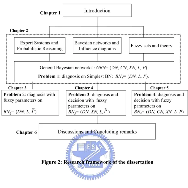
(18) introduced previously, there are four categories of reasoning problems discussed in this dissertation:. 1.. Problem 1: diagnosis with discrete random nodes and crisp parameters. This category. is reasoning from the simplest type of the Bayesian networks, BN1= (DN, L, P), and has been vastly studied in the literatures (Chapter 3). 2.. Problem 2: diagnosis with discrete random nodes and fuzzy parameters in a static. ~ Bayesian network. This kind of problems is reasoning from BN2= (DN, L, P ) (Chapter 3). 3.. Problem 3: diagnosis and decision-making with discrete random nodes and fuzzy. parameters in a static influence diagram. This kind of problems is solved on BN3= ~ (DN, XN, L, P ) (Chapter 4) 4.. Problem 4: diagnosis and decision-making with continuous random nodes, decision. nodes, and crisp parameters in a dynamic influence diagram. This type of problems is answered from BN4= (DN, CN, XN, L, P) (Chapter 5).. For every category of problems, this dissertation first gives a description of problem formulation, and develops the reasoning model in a comprehensive and systematic way. Thereafter, the algorithms and solutions will be designed. One example or examples will be used to illustrate how to operate the reasoning methods, especially in medical informatics and supply chain systems. The outcomes and performances are examined carefully in the discussions. In the final chapter, some concluding remarks will be presented. The conceptual research framework and the dissertation structure are shown in Figure 2.. 8.

(19) Chapter 1. Introduction. Chapter 2. Expert Systems and Probabilistic Reasoning. Bayesian networks and Influence diagrams. Fuzzy sets and theory. General Bayesian networks : GBN= (DN, CN, XN, L, P) Problem 1: diagnosis on Simplest BN: BN1= (DN, L, P). Chapter 3. Chapter 4. Problem 2: diagnosis with fuzzy parameters on ~. BN2= (DN, L, P ). Chapter 6. Chapter 5. Problem 3: diagnosis and decision with fuzzy parameters on ~ BN3= (DN, XN, L, P ). Problem 4: diagnosis and decision with fuzzy parameters on BN4= (DN, CN, XN, L, P). Discussions and Concluding remarks. Figure 2: Research framework of the dissertation. 9.

(20) Chapter 2 Literatures review. This chapter reviews the basic concepts of probabilistic reasoning, Bayesian networks, influence diagrams, and fuzzy sets.. 2.1. Expert systems and probabilistic reasoning First of all, this dissertation defines expert systems as follows.. Definition 2: Expert systems. An expert system can be defined as a computer system (hardware or software) that simulates human experts in a given area of specialization [2]. □ As such, an expert system should be able to process an memorize information, learn and reason in both deterministic an uncertain situations, communicate with human and/or other expert systems, make appropriate decisions, and explains why these decision work. Castillo et al [2] classified the problems that an expert system can deal with into two types: deterministic and stochastic. Deterministic problems can be formulated using a set of rules that relates several well-defined objects. Experts systems that deal with deterministic problems are known as rule-based expert systems. In stochastic or uncertain situations it is necessary to introduce some means for handling uncertainty, such as certainty factors, fuzzy logic, probability, and so on. Expert systems that use probability as a measure of uncertainty are know as probabilistic expert systems, and the strategy they use is know as probabilistic reasoning or probabilistic inference. The ability to use both predictive and diagnostic information is an important component of plausible reasoning, and improper handling of such information leads to strange results. So, Pearl [35] classified the patterns of plausible. 10.

(21) reasoning into abductive reasoning and inductive reasoning. Deduction, or prediction, is a logical process from a hypothesis to deduce evidence where probabilistic relationships are involved [35]. For example, if A is true, then B is true; that is A implies B. Abductive reasoning, or diagnosis, is a logical process that hypothetically explains experimental observations. For example, if A implies B, then finding B is true makes A more credible. George Polya [37] classified plausible reasoning into the following four: 1.. Inductive patterns: “The verification of a consequence renders a conjecture more. credible.” For example, the conjecture “She didn’t sleep well last night” becomes more credible when we verify, “She looks dispirited this morning”. 2.. Successive verification of several consequences: “The verification of a new. consequence counts more or less if the new consequence differs more less from the former, verified consequences.” For example, if in trying substantiating the conjecture “All ravens are black,” we observe n Australian ravens, all of them black, our subsequent confidence in the conjecture will be increased substantially of the (n+1)-th ravens is a black Brazilian rather than another Australian ravens. 3.. Verification of improbable consequences: “The verification of a consequence counts. more or less according as the consequence is more or less improbable in itself.” For example, the conjecture “She didn’t sleep well” obtains more support from “She is nodding this morning” than from the more common observation “She looks dispirited this morning”. 4.. Inference from analogy: “A conjecture becomes more credible when an analogous. conjecture turns out to be true.” For example, the conjecture “Of all objects displacing the same volume, the sphere has the smallest surface” becomes more credible when we prove the relative theorem “Of all curves enclosing the same area, the circle has the shortest perimeter.” This dissertation will focus on the abductive reasoning and decision-making models in 11.

(22) expert systems. In this research, Bayesian networks and influence diagrams play a central role in the uncertainty formalism.. 2.2. Bayesian networks Bayesian networks [34,35] are directed acyclic graphs (DAG) in which the nodes. represent the variables, the arcs represent the direct causal influences between the linked variables, and the strengths of these influences are expressed by forward conditional probabilities. A simple example is given in Figure 1(b). The semantics of Bayesian networks demands a clear correspondence between the topology of a DAG and the dependency relationships portrayed by it. They are widely used knowledge representation and reasoning tools for various domains under uncertainty [1,2,4,8,13-18,20,23,27,34,35]. Influence diagrams are a special type of Bayesian networks with three kinds of nodes: decision nodes, chance nodes, and a value node. Decision nodes, shown as squares, represent choices available to the decision-makers. Chance nodes, shown as circles, represent random variables (or uncertain quantities). Finally, the value node, shown as a diamond, represents the objective (or utility) to be maximized. In a multiple objective decision making model, there may be more than one value nodes. There are two methods for determining the optimal decision policy from an influence diagram [35]. The first, proposed by Howard and Matheson, consists of converting the influence diagram to a decision tree and solving for the optimal policy within the tree, using exp-max labeling procedure. The second approach, proposed by Shachter, to decision-making in influence diagrams consists of eliminating modes from diagram through a series of value-preserving transformations. Several methods have been developed for solving abductive or diagnostic reasoning problems in Bayesian networks. Exact methods exploit the independence structure contained in the network to efficiently propagate uncertainty [2,35]. Meanwhile, stochastic simulation 12.

(23) methods provide an alternative approach suitable for highly connected networks, in which exact algorithms can be inefficient [35]. Recently, search-based approximate algorithms, which search for high probability configurations through a space of possible values, have emerged as a new alternative [36]. On the other hand, two key approaches have been proposed for symbolic inference in Bayesian networks, namely: the symbolic probabilistic inference algorithm (SPI) [38] and symbolic calculations based on slight modifications of standard numerical propagation algorithms [1,2]. The above methods have several limitations for reasoning from a Bayesian network or an influence diagram: 1.. All network nodes or variables must be crisp.. 2.. All relevant parameters are assumed to be crisp.. 3.. Extra constraints or knowledge regarding belief propagation in Bayesian networks are difficult to embed.. 4.. Decision-making and diagnosis cannot be done in a complete model. Even in a compact graphical decision model, like influence diagrams, the proposed methods only focus on maximizing the expected gains but ignoring the problem diagnosis.. Those limitations restrict the usefulness of reasoning in Bayesian networks. First, the conditional probabilities between a node and its parents could be fuzzy parameters because of the difficulties of learning accurately the causal relationships among the nodes. The decision makers may also feel awkward to make judgments for the linguistic vagueness or incomplete knowledge, which make the probability theory not suitable in problem formulation. Under such circumstances, the fuzzy nodes in a Bayesian networks can be introduced to overcome the obstacle. Additionally, knowledge workers often acquire additional information regarding inferences in Bayesian networks, particularly when facing diverse diagnostic scenarios. This. 13.

(24) information can relate to boundary, dependency or disjunctive conditions.. 2.3. Fuzzy sets and theory Fuzzy sets were introduced by Zadeh [43] in 1965 to manipulate data and information. processing uncertainties which statistics is not proper for use. It was particularly designed to mathematically represent uncertainty as well as vagueness and to offer formalized tools for handling the imprecision intrinsic to many domains. Fuzzy sets are a means of representing and manipulating information not precise. A fuzzy subset Ã of a set X can be can be defined as a set of ordered pairs, each with the first element from X and the second element from the interval [0,1], with exactly one ordered pair for each element of X. This defines a mapping as below.. µ A~ : X → [0,1] , between elements of the set X and values in the interval [0,1]. The value zero is to represent complete non-membership, the value one is to represent complete membership, and values in between are to represent intermediate degrees of membership. The set X is referred as the universe of discourse for the fuzzy subset Ã. Usually, the mapping µ A~ is described as a function, the membership function of Ã. The degree to which the statement “x is in Ã” is true is determined by finding the ordered pair (x, µ A~ ). The degree of the statement to be true is the second element of the ordered pair.. Definition 3: Fuzzy membership functions.. Let X be a nonempty set. A fuzzy set Ã in X is characterized by its membership function. µ A~ : X → [0,1] , and µ A~ is interpreted as the degree of membership of element x in fuzzy set Ã for each x □ 14.

(25) Visibly, Ã is completely determined by the following expression.. ~ A = {( x, µ A~ ( x)) | x ∈ X } . By the above expression, the terms membership function and fuzzy subset are used interchangeably. A fuzzy subset Ã of a classical set X is called normal if there exists an. x ∈ X such that Ã(x) = 1. Otherwise, Ã is subnormal. An α-level set (or α-cut) of a fuzzy set Ã of X is a non-fuzzy set denoted by [Ã]α and defined by. {. }. ~ ⎧ x ∈ X | A( x) ≥ α , ~ [ A]α = ⎨ ~ ⎩cl(supp A),. if α > 0 if α = 0. ~ where cl(supp A) denotes the closure of the support of Ã. A fuzzy set Ã of X is called convex if [Ã]α is a convex subset of X for all α ∈ [0,1] . Similarly, a fuzzy number can be defined as follow.. Definition 4: Fuzzy numbers. A fuzzy number Ã is a fuzzy set of the real line with a normal, fuzzy convex and ~ continuous membership function satisfying the limit conditions, and lim A(t ) = 0 .□ t → −∞. Based on the concepts reviewed in this chapter, next chapter will show how this dissertation solves the fuzzy reasoning problems on Bayesian network.. 15.

(26) Chapter 3 Diagnosis with fuzzy parameters. Based on the review in Chapter 2, we understand that current adductive reasoning methods can solve very limited scope of the reasoning from Bayesian networks. This chapter will first illustrate the steps to solve a traditional abductive reasoning query, and then develop the model for diagnosis with crisp nodes and fuzzy parameters in Bayesian network.. 3.1. Reasoning with crisp information In this section, a simplest form of abductive reasoning is introduced as follow.. Problem 1: Given the evidence set Ĕ from BN1= (DN, L, P), compute the belief distribution. of Û ⊂ BN1\ Ĕ, BEL(Û| Ĕ). ▓. Problem 1 is interpreted with the following case from medicine and Example 1.. Consider the following example from Pearl [35]. “Metastatic cancer is a possible cause of a brain tumor and is an explanation for increased total serum calcium. Either of these could explain a patient falling into a coma. Severe headache is also possibly associated with a brain tumor.” Figure 1(b) shows a Bayesian network representing the above cause and effect relationships. Table 1 lists the causal influences in terms of conditional probability distributions. Each variable is characterized by the probability given the state of its parents. For instance: C ∈{1,0} represents the dichotomy between having a brain tumor and not having one, +c denotes the assertion C = 1 or “Brain tumor is present”, and –c is the negation of +c, namely, C = 0. The root node, A, which has no parent, is characterized by its prior. 16.

(27) probability distribution. The above information can be used to solve the following reasoning problems.. Example 1: Compute the posterior probability of every A, B, and C, given the conditional. probabilities in Table 1, and a situation involving a patient who is suffering from a severe headache (E=1) but has not fallen into a coma (D=0); that is, compute P(a|-d, +e), P(b|-d, +e) and P(c|-d, +e). □. Now this section reviews one conventional method, clustering, for computing the posterior probabilities with crisp parameters and no extra constraints. Consider the Bayesian network in Figure 1(b) with the crisp information in Table 1. Clustering [2,35] can transform Figure 1(b) into an equivalent tree structure in Figure 1(c), where nodes B and C are collapsed into a compound node Z = B & C . Let Z = {z1 , z 2 , z3 , z 4 } be a set of cardinalities of Z and z1 = ( +b,+ c) , z 2 = (-b,+ c ) , z3 = (+b,-c) , and z 4 = (-b,-c ) . Moreover, let WY denote the state of all variables except Y; for example, W A ={ ( z1 ,-d + e) , ( z 2 ,-d + e) , ( z3 ,-d + e) , ( z 4 ,-d + e) }. From Pearl [35], the value of P ( y | WY ) , which is the distribution of y. conditioned on the value WY , can be calculated as below considering every instance of y.. 17.

(28) 4 ⎫ P (+ a | W A ) = α A P ( + a )∑ P ( zi | + a ) P ( − d | zi ) P ( + e | zi ) ⎪ i =1 ⎪ 4 ⎪ P (− a | W A ) = α A P (−a )∑ P( zi | −a ) P(−d | zi ) P(+ e | zi ) ⎪ i =1 ⎪ 1 ⎪ P (+b | WB ) = α B ∑ [ P(a) ∑ P( zi | a) P(−d | zi ) P(+ e | zi )] ⎪ a =0 i =1,3 ⎪ ⎬ 1 P (−b | WB ) = α B ∑ [ P (a ) ∑ P( zi | a) P(−d | zi ) P(+ e | zi )]⎪ ⎪ a =0 i = 2, 4 ⎪ 1 P (+ c | WC ) = α C ∑ [ P(a ) ∑ P( zi | a ) P (−d | zi ) P(+ e | zi )]⎪⎪ a =0 i =1, 2 ⎪ 1 ⎪ P (−c | WC ) = α C ∑ [ P(a ) ∑ P( zi | a ) P(−d | zi ) P(+ e | zi )]⎪ a =0 i =3, 4 ⎭. (1). where α A , α B , and α C are the normalizing constant ensuring that P ( + a | W A ) + P (-a | W A ) = 1 P(+b | WB ) + P(-b | WB ) = 1. (2). P(+ c | WC ) + P(-c | WC ) = 1 From (2), then intuitively. α = α A = α B = αC =. 1 1. 4. a =0. i =1. (3). ∑ P ( a )∑ P ( zi | a ) P ( −d | zi ) P ( + e | zi ). and. α ∑∑ P(a) P( zi | a) P(−d | zi ) P(+e | zi ) = 1 a. (4). zi. The value of P ( + a | W A ) in (1) is obtained below for the data in Table 1: P(+ a | W A ) = α (.2)[(.8)(.2)(1 − .8)(.8) + (1 − .8)(.2)(1 − .8)(.8) + (.8)(1 − .2)(1 − .8)(.6) + (1 − .8)(1 − .2)(1 − .05)(.6)]. .. Similarly, P(− a | W A ) = α (1 − .2)[(.2)(.05)(1 − .8)(.8) + (1 − .2)(.05)(1 − .8)(.8) + (.2)(1 − .05)(1 − .8)(.6) + (1 − .2)(1 − .05)(1 − .05)(.6)]. .. From (1) and (3), then α = 2.432 , P ( + a | W A ) =0.097, and P ( − a | W A ) =0.903.. 18.

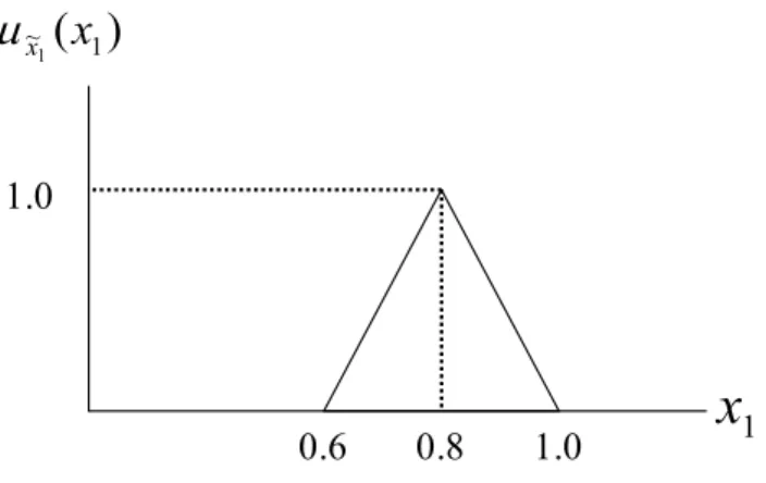
(29) The answers to Example 1 are. P(a | −d ,+e) = (0.097,0.903) , P(b | −d ,+e) = (0.097,0.903) , P(c | −d ,+e) = (0.031,0.969) . █. Observing the solution stated above, several limitations persist in the conventional reasoning methods. First, all network nodes and relevant parameters are assumed to be crisp. This narrows the usefulness of reasoning methods when some parameters are hard to estimate. Freeling [7] claimed fuzzy probability as an extension of probability theory, which is more promising than possibility and probability theory as a decision aid. Second, extra constraints or knowledge regarding belief propagation in Bayesian networks are difficult to embed. Third, different reasoning tasks, such as diagnosis as well as treatment planning, cannot be completed in the same place. Those attributes are often needed in both business and medical informatics. Furthermore, the limitations encumber reasoning to be automated. For some systematic or technical reasons, the conditional probabilities of the network nodes may be fuzzy, instead of crisp. For instance, P(+b | + a) cannot be 0.8 but rather is a fuzzy number, say ~ x1 , where P ( +b | + a ) = ~ x1 , and is associated with a membership function. µ ~x1 ( x1 ) , represented as follows. (See Figure 3) µ ~x1 ( x1 ) = 5( x1 − 0.6) − 5( x1 − 0.8 + x1 − 0.8),. 0.6 ≤ x1 ≤ 1. where “ ∗ ” denotes the absolute value of a term *.. 19.

(30) µ ~x ( x1 ) 1. 1.0. 0.6. 0.8. x1. 1.0. Figure 3: The membership function µ ~x1 ( x1 ) of ~ x1. The above expression and Figure 3 mean that the domain of ~ x1 is between 0.6 and 1.0. If x1 =0.8 then µ ~x1 ( x1 ) =1, implying that x1 =0.8 is the most possible situation. If x1 ≤ 0.6 or x1 ≥ 1 then µ ~x1 ( x1 ) =0, the least possible manifestation of x1 . If x1 =0.7, then. µ ~x1 ( x1 ) =0.5.. µ ~x ( x7 ) 7. 1.0. 0.7. 0.8. 0.85. 0.95. x7. Figure 4: The membership function µ ~x7 ( x7 ) of ~ x7. Fuzzy membership functions can be expressed in various ways. For example, let x7 P(+d|+b,+c) = ~. and express µ ~x7 ( x7 ) as the following function (Figure 4). 20.

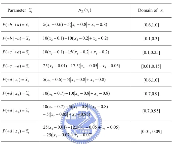
(31) µ ~x7 ( x7 ) = 10( x7 − 0.7) − 5( x7 − 0.8 + x7 − 0.8) − 5( x7 − 0.85 + x7 − 0.85),. 0.7 ≤ x7 ≤ 0.95. .. µ ~x7 ( x7 ) is a trapezoid membership function and comprises four line segments, where 0.8 ≤ x7 ≤ 0.85 has the maximal membership.. 3.2. Problem and goals This chapter discusses reasoning with crisp nodes and fuzzy parameters as the. following problem.. ~ Problem 2: Given the evidence set Ĕ from BN2= (DN, L, P ), compute the belief distribution of Û ⊂ BN2\ Ĕ, BEL(Û| Ĕ).▓. xi , i = 1,2,...,8 , where P(+b|+a) = ~ The fuzzy parameters are denoted by as ~ x1 , x3 , P(+c|-a) = ~ x5 , P(+d|-b, +c) = ~ x6 , P(+d|+b, P(+b|-a) = ~ x 2 , P(+c|+a) = ~ x 4 , P(+d|+b,+c) = ~ x7 , and P(+d|-b, -c) = ~ x8 . Table 2 lists the membership functions of the fuzzy -c) = ~ parameters, among which µ ~x7 ( x7 ) and µ ~x8 ( x8 ) are trapezoid membership functions while the remainder are triangular functions. After introducing the fuzzy probabilities, the Example 1 turns into a more complex problem as Example 2.. 21.

(32) Table 2: The membership functions of fuzzy probabilities. Parameter ~ xi. µ ~xi ( xi ). Domain of xi. P (+b | + a ) = ~ x1. 5( x1 − 0.6) − 5( x1 − 0.8 + x1 − 0.8). [0.6,1.0]. P (+b | − a ) = ~ x2. 10( x2 − 0.1) − 10( x2 − 0.2 + x2 − 0.2). [0.1,0.3]. P(+c | + a ) = ~ x3. 10( x3 − 0.1) − 15( x3 − 0.2 + x3 − 0.2). [0.1,0.25]. P (+ c | − a ) = ~ x4. 25( x 4 − 0.01) − 17.5( x 4 − 0.05 + x 4 − 0.05). [0.01,0.15]. P(+ d | z1 ) = ~ x5. 5( x5 − 0.6) − 5( x5 − 0.8 + x5 − 0.8). [0.6,1.0]. P(+ d | z 2 ) = ~ x6. 10( x6 − 0.7) − 10( x6 − 0.8 + x6 − 0.8). [0.7,0.9]. P(+ d | z 3 ) = ~ x7. P(+ d | z 4 ) = ~ x8. 10( x 7 − 0.7) − 5( x 7 − 0.8 + x 7 − 0.8) − 5( x7 − 0.85 + x7 − 0.85). 25( x8 − 0.01) − 12.5( x8 − 0.05 + x8 − 0.05). − 25( x8 − 0.07 + x8 − 0.07). [0.7,0.95]. [0.01, 0.09]. Example 2: Compute the belief distributions P(a|-d, +c), P(b|-d, +c), and P(c|-d, +c), given. the fuzzy membership functions in Table 2 and some constraints related to belief propagation.. Current abductive reasoning methods have difficulties in solving Problem 2 and Example 2 since it involves fuzzy information and extra constraints. Consider abductive reasoning with constraints. For a given Bayesian network, knowledge workers (such as clinicians) may have professional judgments regarding the features of certain nodes and the relationships among them in particular diagnostic backgrounds. These features and relationships can take the form of various constraints [26].. 22.

(33) 1.. Boundary constraints: From additional information or observations, clinicians can infer that the posterior probability of A given E=1 and D=0 should be higher than 0.1 but lower than 0.3, which is expressed as. 0.1 ≤ P(+ a | -d ,+e) ≤ 0.3 2.. (5). Functional dependency: The beliefs of certain nodes are functionally dependent. For example, clinicians can judge that the posterior probability of B is roughly a certain multiple of that of A given E=1 and D=0, which is expressed as. P ( + a | - d , + e) ≤ 2 P ( + b | - d , + e) 3.. (6). Disjunctive constraints: Sometimes disjunction may occur between nodes. For example, a doctor may estimate that either P(+ a | -d ,+e) or P(+b | -d ,+e) is equal to or below 0.2, which is expressed as Either P(+ a | -d ,+e) ≤ 0.2 or P(+b | -d ,+e) ≤ 0.2. (7). By introducing these constraints into the reasoning system, the following problems are formulated.. Example 2.1: Compute the belief distributions P(a|-d, +e), P(b|-d, +e), and P(c|-d, +e), given. the fuzzy membership functions in Table 2 and the following constraints.. 0.1 ≤ P(+ a | -d ,+e) ≤ 0.3 , P ( + b | -d , + e ) ≤ 2 P ( + c | - d , + e ) Either P(+ a | -d ,+e) ≤ 0.2 or P(+b | -d ,+e) ≤ 0.2 .. Example 2.1 is more complicated and difficult than Example 1 when solved using. 23.

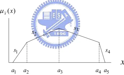
(34) current propagation methods.. 3.3. Model development The following illustrates another approach for calculating the posterior probabilities. with fuzzy parameters.. 3.3.1. Fuzzy parameters. x , as displayed in Figure 5. This Consider a membership function µ ~x ( x) of ~ piecewise linear function generally is expressed as. µ ~x ( x) s3. s2 s1. s4. x a1. a2. a3. a4 a5. Figure 5: A membership function of fuzzy probability. ⎧s1 ( x − a1 ), ⎪µ (a ) + s ( x − a ), 2 2 2 ⎪⎪ µ ~x ( x) = ⎨µ (a3 ) + s3 ( x − a3 ), ⎪µ (a ) + s ( x − a ), 4 4 4 ⎪ ⎩⎪0,. a1 < x ≤ a2 a 2 < x ≤ a3 a3 < x ≤ a 4 a 4 < x ≤ a5 elsewhere.. (8). Computing the above expression is complex. Consequently, this work employs an efficient method of expressing a piecewise linear function. Consider the following. 24.

(35) proposition.. x , as displayed Proposition 1 Let µ ~x ( x) denote the membership function of fuzzy variable ~ in Figure 4, where a j , j = 1,2,..., m represent the break points of µ ~x ( x) , and s j , j = 1,2,..., n are the slopes of line segments between a j and a j +1 , and µ ~x ( x) is the sum of absolute terms [24,40]:. µ ~x ( x ) = µ ( a1 ) + s1 ( x − a1 ) +. si − si −1 ( x − aj + x − aj) 2 j=2 m. ∑. (9). If µ ~x ( x) in (9) is to be maximized, then the following proposition is used for convenient linearization.. Proposition 2 Maximizing a function µ ~x ( x) in (9) requires solving the following linear. program [24,40]: j ⎫ si − si −1 ( x − a j + ∑ d k )⎪ 2 j =2 k =1 ⎪ ⎪ subject to ⎪ x + d1 ≥ a2 , ⎪ ⎪ x + d1 + d 2 ≥ a3 , ⎪⎪ # ⎬ ⎪ x + d1 + d 2 + " + d m−1 ≥ am , ⎪ 0 ≤ d1 ≤ a2 , ⎪ ⎪ 0 ≤ d k −1 ≤ ak − ak −1 , for k = 2,3, " , m, ⎪ ⎪ x ∈ F ( feasible set ). ⎪ ⎪⎭. Max. m. z = s1 ( x − a1 ) + 2 ∑. Proof:. Since d k −1 ≤ ak − ak −1 , then clearly x ≥ ak − (d1 + d 2 + " + d k −1 ) ≥ ak −1 − (d1 + d 2 + " + d k −2 ) , so constraint. 25. (10).

(36) x + d1 + d 2 + " + d k −2 ≥ ak −1 is converted by constraint x + d1 + d 2 + " + d k −2 + d k −1 ≥ ak , for k = 2,3,", m . █. From Proposition 2, the non-linear membership functions are transformed into equivalent linear functions.. 3.3.2. Fuzzy Abductive Models. To compute the belief distribution of the unknown nodes in a Bayesian networks with fuzzy parameters, there are several alternative objective functions. Consider Example 2.1. 1.. Estimate the upper/ lower bound for P(+a|-d, +e), P(+b|-d, +e), P(+c|-d, +e) by maximizing/ minimizing the beliefs, respectively. e.g. Maximize P(+a|-d, +e) → Upper bound of P(+a|-d, +e), Minimize P(+a|-d, +e) → Lower bound of P(+a|-d, +e).. 2.. Generate a pair of belief, e.g. (P(+a|-d, +e)min µ, P(+a|-d, +e)max µ) with respect to the maximal/ minimal confidence for fuzzy parameters. e.g. Maximize µ ~xi ( xi ) → under maximal confidence for fuzzy parameters. Minimize µ ~xi ( xi ) → under minimal confidence for fuzzy parameters.. 3.. Generate the distributions of P(+a|-d, +e), P(+b|-d, +e), P(+c|-d, +e) by α-cut and fuzzy simulation.. All the above classes of the objectives can be implemented based on the decision-makers’ needs or preferences. This dissertation chooses the second class as the 26.

(37) objectives. Since there are several fuzzy parameters involved in Problem 2, this dissertation will estimate the belief distribution for the unknown nodes with the maximal and minimal confidence. The belief distribution under maximal confidence will be estimated by maximizing the fuzzy membership functions; oppositely, the belief distribution under minimal confidence will be estimated by minimizing the fuzzy membership function. Building upon the clustering method, Proposition 1 and 2, the abductive model for solving Example 2.1 is formulated below.. Model 1(a) (for maximal confidence) Maximize µ ~xi ( xi ), i = 1,2,",8,. subject to (1), 0.1 ≤ P(+ a | -d ,+e) ≤ 0.3, P(+b | -d ,+e) ≤ 2 P(+c | -d ,+e), Either P(+ a | -d ,+e) ≤ 0.2 or P(+b | -d ,+e) ≤ 0.2,. (11). Model 1(b) (for minimal confidence). Minimize µ ~xi ( xi ), i = 1,2,",8, subject to (1), 0.1 ≤ P(+ a | -d ,+e) ≤ 0.3, P(+b | -d ,+e) ≤ 2 P(+c | -d ,+e), Either P(+ a | -d ,+e) ≤ 0.2 or P(+b | -d ,+e) ≤ 0.2,. (12). where the objective function maximize and minimize all fuzzy membership functions. Since 27.

(38) (4) contains numerous non-separate nonlinear terms, Model 1 is a highly non-linear and nonconvex program. This dissertation will deal with the disjunctive constraint first and takes care of the nonlinear issue in the following proposition.. x ) ≤ 0 or g ( ~ x ) ≤ 0 can be expressed by the Proposition 3 A disjunctive constraint f ( ~ following inequalities. M (θ 1 − 1) ≤ f ( ~ x ) ≤ Mθ 1 + M (1 − θ 2 ),⎫ ⎪ M (θ 2 − 1) ≤ g ( ~ x ) ≤ Mθ 2 + M (1 − θ 1 ) ⎬ ⎪ ε ≤ θ 2 + θ 1 ≤ 1. ⎭. (13). where θ 1 and θ 2 are 0-1 variables, M is a relatively large number, and ε is a relatively small positive number. The four possible combinations of θ 1 and θ 2 can be checked as follows: (i) for θ 1 = 1, x ) ≤ M and 0 ≤ g ( ~ x ) ≤ M , which are inactive constraints; θ 2 =1 the constraints are 0 ≤ f ( ~ (ii) for θ1 = 0, θ 2 =1 then − M ≤ f ( ~ x ) ≤ 0 and 0 ≤ g ( ~ x ) ≤ 2M , meaning that when g (~ x ) ≥ 0 , f (x~ ) must be 0 or less; (iii) for θ1 = 1, θ 2 =0, the constraints are 0 ≤ f ( ~ x ) ≤ 2M. x ) ≤ 0 , which implies that when f ( ~ x ) ≥ 0 , g (x~ ) must be 0 or less; (iv) for and − M ≤ g ( ~ x ) ≤ M , which are θ1 = 0, θ 2 =0 the constraints become − M ≤ f ( ~x ) ≤ M and − M ≤ g ( ~ inactive constraints. The third constraint in (13) excludes the combinations θ1 = 1, θ 2 =1 and x ) ≤ 0 or g ( ~ x ) ≤ 0 must be θ1 = 0, θ 2 =0. To summarize, (13) implies that either f ( ~ satisfied.. 3.4. Solution and illustrative examples Abductive reasoning problems in certain applications are solved below using the. proposed constrained optimization approach. 28.

(39) Example 2.1 is solved using the following program. Maximize µ ~xi ( xi ), i = 1,2,",8, (for the maximal confidence), or Minimize µ ~xi ( xi ), i = 1,2,",8, (for the minimal confidence),. ⎫ ⎪ µ ~x1 ( x1 ) = 5( x1 − 0.6) − 5( x1 − 0.8 + x1 − 0.8), ⎪ ⎪ µ ~x2 ( x2 ) = 10( x2 − 0.1) − 10( x2 − 0.2 + x2 − 0.2), ⎪ ⎪ µ ~x3 ( x3 ) = 10( x3 − 0.1) − 15( x3 − 0.2 + x3 − 0.2), ⎪ ⎪ µ ~x4 ( x4 ) = 25( x4 − 0.01) − 17.5( x4 − 0.05 + x4 − 0.05), ⎪ ⎬ µ ~x5 ( x5 ) = 5( x5 − 0.6) − 5( x5 − 0.8 + x5 − 0.8), ⎪ ⎪ µ ~x6 ( x6 ) = 10( x6 − 0.7) − 10( x6 − 0.8 + x6 − 0.8), ⎪ µ ~x7 ( x7 ) = 10( x7 − 0.7) − 5( x7 − 0.8 + x7 − 0.8) − 5( x7 − 0.85 + x7 − 0.85),⎪ ⎪ ⎪ µ ~x8 ( x8 ) = 25( x8 − 0.01) − 12.5( x8 − 0.05 + x8 − 0.05) ⎪ − 25( x8 − 0.07 + x8 − 0.07), ⎪⎭. s.t.. (14). α [0.2 x1 x3 (1-~x5 )0.8 + 0.2(1-~x1 ) ~x3 (1-~x6 )0.8. ⎫ ⎪ ⎪ ⎪ 2 4 5 2 4 6 ⎪ x2 (1 - ~ x4 )(1 - ~ x7 )0.6 + 0.8(1 - ~ x2 )(1 - ~ x4 )(1 - ~ x8 )0.6] = 1,⎪ + 0.8 ~ ⎬ 0.1 ≤ P(+ a | -d ,+e) ≤ 0.3, ⎪ ⎪ P(+b | -d ,+e) ≤ 2 P(+ c | -d ,+e), ⎪ Either P(+ a | -d ,+e) ≤ 0.2 or P(+b | -d ,+e) ≤ 0.2, ⎪ ~ ⎪ xi ∈ F ( feasible set ). ⎭ x1 (1 - ~ x3 )(1 - ~ x7 )0.6 + 0.2(1 - ~ x1 )(1 - ~ x3 )(1 - ~ x8 )0.6 + 0.2 ~ ~ ~ ~ ~ ~ ~ + 0.8 x x (1 - x )0.8 + 0.8(1 - x ) x (1 - x )0.8. (15). First (14) is linearized using Proposition 2 and then the initial program is altered into the equivalent program as follows. Maximize µ ~xi ( xi ), i = 1,2,",8, (for the maximal confidence), or Minimize µ ~xi ( xi ), i = 1,2,",8, (for the minimal confidence),. s.t. 29.

(40) µ ~x1 ( x1 ) = 5( x1 − 0.6) − 2[5( x1 − 0.8 + d1 )],. ⎫ ⎪ µ ~x2 ( x2 ) = 10( x2 − 0.1) − 2[10( x2 − 0.2 + d 2 )], ⎪ ⎪ µ ~x3 ( x3 ) = 10( x3 − 0.1) − 2[15( x3 − 0.2 + d 3 )], ⎪ ⎪ µ ~x4 ( x4 ) = 25( x4 − 0.01) − 2[17.5( x4 − 0.05 + d 4 )], ⎪ µ ~x5 ( x5 ) = 5( x5 − 0.6) − 2[5( x5 − 0.8 + d 5 )], ⎪ ⎪ µ ~x6 ( x6 ) = 10( x6 − 0.7) − 2[10( x6 − 0.8 + d 6 )], ⎪ ⎪ µ ~x7 ( x7 ) = 10( x7 − 0.7) − 2[5( x7 − 0.8 + d 71 ) + 5( x7 − 0.85 + d 71 + d 72 )], ⎪ µ ~x8 ( x8 ) = 25( x8 − 0.01) − 2[12.5( x8 − 0.05 + d 81 ) + 25( x82 − 0.07 + d 81 + d 82 )],⎪⎬ ⎪ x1 + d1 ≥ 0.8, 0 ≤ d1 ≤ 0.8, ⎪ x2 + d 2 ≥ 0.2, 0 ≤ d 2 ≤ 0.2, ⎪ ⎪ x3 + d 3 ≥ 0.2, 0 ≤ d 3 ≤ 0.2, ⎪ ⎪ x4 + d 4 ≥ 0.05, 0 ≤ d 4 ≤ 0.05, ⎪ x5 + d 5 ≥ 0.8, 0 ≤ d 5 ≤ 0.8, ⎪ ⎪ x6 + d 6 ≥ 0.8, 0 ≤ d 6 ≤ 0.8, ⎪ x7 + d 71 + d 72 ≥ 0.85, 0 ≤ d 71 ≤ 0.8, , 0 ≤ d 72 ≤ 0.05, ⎪ ⎪ x8 + d 81 + d 82 ≥ 0.07, 0 ≤ d 81 ≤ 0.05, , 0 ≤ d 82 ≤ 0.02, and (15) ⎭. (16). To ensure belief propagation the lower bound of the membership functions is set at 0.2; that is, the membership of every fuzzy parameter must equal or exceed 0.2, which excludes scenarios involving poorly estimated parameters. LINGO 8.0 solves Example 2.1 in less than one second. The solutions for maximal confidence are α =2.6743 and 4. P(+ a | + d ,−e) = αP(+ a)∑ P( zi | + a) P(− d | zi ) P(+ e | zi ) =0.1097, i =1. P ( + b | + d , − e) = α. ∑ [ P(a) ∑ P( zi | a) P(−d | zi ) P(+e | zi )] =0.20,. a =0,1. P ( + c | + d , − e) =. i =1,3. +a. ∑ [ P(a) ∑ P( zi | a) P(−d | zi ) P(+e | zi )] =0.1.. a =0,1. i =1, 2. The solutions for minimal confidence are. 30.

(41) 4. P(+ a | + d ,−e) = αP(+ a)∑ P( zi | + a) P(− d | zi ) P(+ e | zi ) =0.1056, i =1. P ( + b | + d , − e) = α. ∑ [ P(a) ∑ P( zi | a) P(−d | zi ) P(+e | zi )] =0.2,. a =0,1. P ( + c | + d , − e) =. i =1,3. +a. ∑ [ P(a) ∑ P( zi | a) P(−d | zi ) P(+e | zi )] =0.1. a =0,1. □. i =1, 2. Table 3 lists the detailed solutions. The results of this model differ from those for Example 1. In Table 3, P(+ a | + d ,−e) changes to [0.1056, 0.1058], where 0.1056 and 0.1058 is solved by minimizing and maximizing the fuzzy membership functions, respectively. P(+b | + d ,−e) changes to 0.2, and P(+b | + d ,−e) changes to 0.1, which implies that the solutions are insensitive to the confidence of fuzzy parameters. This variance results from the constraints that dominate the belief propagation. Readers may have deduced that Example 1 can be considered a special case in which every membership of the fuzzy parameters converges on 1.. 31.

(42) Table 3: Solution of Example 2.1 Under maximal confidence. Under minimal confidence. BEL(a +). 0.1058. 0.1056. BEL(b+ ). 0.20. 0.2. BEL(c + ). 0.10. 0.10. x1. 0.9449. 0.96. x2. 0.2762. 0.28. x3. 0.2339. 0.2062. x4. 0.1284. 0.1300. x5. 0.6458. 0.64. x6. 0.7265. 0.72. x7. 0.7321. 0.7405. x8. 0.0831. 0.0860. µ ~x ( x1 ). 0.2755. 0.2. µ ~x ( x 2 ). 0.2383. 0.2. µ ~x ( x3 ). 0.3218. 0.2. µ ~x ( x 4 ). 0.2162. 0.2. µ ~x ( x5 ). 0.2290. 0.2. µ ~x ( x6 ). 0.2651. 0.2. µ ~x ( x7 ). 0.2496. 0.2. µ ~x ( x8 ). 0.3441. 0.2. 1. 2. 3. 4. 5. 6. 7. 8. 32.

(43) Under certain circumstances, knowledge workers may need to compromise among diverse, even conflicting information sources, causing fuzzy parameters to differ from their most possible values.. Example 2.2 (Just-in-time techniques and firm performance): This example uses the. Bayesian network to model the relationship between just-in-time purchasing techniques and firm performance [10]. Just-in-time purchasing (JITP) is an important component of supply chain management in managing inventory flows. Several key factors link the JITP process and firm performance, and Figure 6 models the relationships among these factors. Tables 4 and 5 summarize the probability distributions of the nodes and fuzzy parameters. This study hypothesizes a scenario in which inventory management performance is good ( im + ), employ relationship is poor ( er − ), transportation performance is good ( ta + ), and financial and market performance is poor ( fm − ). The problem involves calculating the belief distribution of all unknown nodes, top management commitment ( tp ), supplier value-added ( su ), training ( tr ), quantity delivered ( qd ), and time-based quality performance ( tq ). The reasoning model is formulated as (17).. 33.

(44) Top Management Commitment. Supplier Value-added. Transportation. TP. TR. SU. TA. ER. Quantities Delivered Inventory Management Performance. Training. Employee Relations. TQ. QD. Time-based Quality Performance. IM. FM. Financial & Market Performance. Figure 6: A Bayesian network of the relationships between JITP techniques and performance measures [10]. Table 4: The conditional probability distribution of Example 2.2. P(tp +) = ~ x31 P( su + | tp +) = ~ x32 ~ P(tr + | tp +) = x. P( su + | tp −) = ~ x33 ~ P(tr + | tp −) = x. P(ta + | su +) = 0.7 P(qd + | su + ) = 0.8 P(im+ | qd +) = 0.3 P(tq + | su +) = 0.4 P( fm+ | tq +) = 0.7 P(er + | tr +) = 0.6. P(ta + | su −) = 0.1 P(qd + | su −) = 0.3 P(im+ | qd −) = 0.1 P(tq + | su −) = 0.05 P( fm+ | tq −) = 0.1 P(er + | tr −) = 0.1. 34. 35. 34.

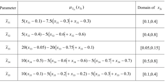
(45) Table 5: The membership functions of fuzzy probabilities in Example 2.2.. µ ~x3i ( x3i ). Parameter. Domain of x3i. ~ x31. 5( x31 − 0.1) − 7.5( x31 − 0.3 + x31 − 0.3). [0.1,0.4]. ~ x32. 5( x32 − 0.4) − 5( x32 − 0.6 + x32 − 0.6). [0.4,0.8]. ~ x33. 20( x33 − 0.05) − 20( x33 − 0.75 + x33 − 0.1). ~ x34. 10( x34 − 0.5) − 5( x34 − 0.6 + x34 − 0.6) − 5( x34 − 0.7 + x34 − 0.7). [0.5,0.8]. ~ x35. 10( x35 − 0.1) − 5( x35 − 0.2 + x35 − 0.2) − 5( x35 − 0.3 + x35 − 0.3). [0.1,0.4]. Maximize. µ ~x3i ( x3i ) (for the maximal confidence), or. Minimize. µ ~x3i ( x3i ) (for the minimal confidence),. [0.05,0.15]. s.t.. µ ~x31 ( ~x31 ) = 5( x31 − 0.1) − 7.5( x31 − 0.3 + x31 − 0.3), µ ~x32 ( x32 ) = 5( x32 − 0.4) − 5( x32 − 0.6 + x32 − 0.6), µ ~x33 ( x33 ) = 20( x33 − 0.05) − 20( x33 − 0.75 + x33 − 0.1), µ ~x34 ( x34 ) = 10( x34 − 0.5) − 5( x34 − 0.6 + x34 − 0.6) − 5( x34 − 0.7 + x34 − 0.7), µ ~x35 ( x35 ) = 10( x35 − 0.1) − 5( x35 − 0.2 + x35 − 0.2) − 5( x35 − 0.3 + x35 − 0.3), α ∑∑∑∑∑ [ P(tp ) P(tr | tp ) P( su | tp ) P(ta + | su ) P(qd | su ) P(tq | su ) tp su tr qd tq. × P(er − | tr ) P(im + | qd ) P( fm − | tq )] = 1, P(tp + | ta +, er −, im +, fm −) > 0.6, P( su + | ta +, er −, im +, fm −) > 0.8.. First the nonlinear membership functions are linearized, yielding (18). Maximize. µ ~x3i ( x3i ) (for the maximal confidence), or 35. (17).

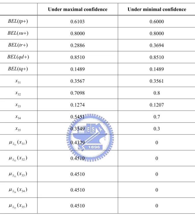
(46) Minimize. µ ~x3i ( x3i ) (for the minimal confidence),. s.t.. µ ~x31 ( x31 ) = 5( x31 − 0.1) − 2[7.5( x31 − 0.3 + d 31 )], µ ~x32 ( x32 ) = 5( x32 − 0.4) − 2[7.5( x32 − 0.6 + d 32 )], µ ~x33 ( x33 ) = 20( x33 − 0.05) − 2[20( x33 − 0.1 + d 33 )], µ ~x34 ( x34 ) = 10( x34 − 0.5) − 2[5( x34 − 0.6 + d 341 ) + 5( x34 − 0.7 + d 342 )], µ ~x35 ( x35 ) = 10( x35 − 0.1) − 2[5( x35 − 0.2 + d 351 ) + 5( x35 − 0.3 + d 352 )],. (18). α ∑∑∑∑∑ [ P(tp ) P(tr | tp ) P( su | tp ) P(ta + | su ) P(qd | su ) P(tq | su ) tp su tr qd tq. × P (er − | tr ) P(im + | qd ) P( fm − | tq )] = 1, P (tp + | ta +, er −, im +, fm −) > 0.6, P ( su + | ta +, er −, im +, fm −) > 0.8.. LINGO 8.0 solves the above program in approximately 5 seconds, obtaining the following results For the model under the maximal confidence:. α =30.5359, P(tp + | ta +, er −, im+, fm−) = 0.6103, P( su + | ta +, er −, im+, fm−) = 0.8, P(tr + | ta +, er −, im+, fm −) = 0.2886, P(qd + | ta +, er −, im+, fm−) = 0.8510, P(tq + | ta +, er −, im+, fm−) = 0.1489. For the model under the minimal confidence:. α =30.9791, P(tp + | ta +, er −, im+, fm−) = 0.6000, P( su + | ta +, er −, im+, fm−) = 0.8, P(tr + | ta +, er −, im+, fm −) = 0.3695, P(qd + | ta +, er −, im+, fm−) = 0.8510, P(tq + | ta +, er −, im+, fm−) = 0.1489. Table 6 lists the details.. 36.

(47) 3.5. Discussions and conclusions This chapter develops a non-linear programming model for dealing with constrained. abductive reasoning on Bayesian networks. This model can be built on any exact propagation methods in Bayesian networks. The present study involves some fuzzy parameters and certain extra constraints. Optimization techniques, including piecewise linearization, are adopted to solve this non-linear programming model and obtain the solutions to the abductive reasoning problems under maximal and minimal confidence to the fuzzy parameters. Since the constraints in this model are extremely non-linear, and numerous non-separable terms are involved, local optima are obtained at the present stage. To enhance the solution quality, some global optimization techniques [24,40,41] can be further used for extended studies. Simultaneously, various reasoning related constraints are considered, including boundary constraints, dependency and disjunctive constraints. Compared to traditional methods that deal with constraints by dummy auxiliary nodes [8, 10], this optimization model of abduction avoids network restructuring. All extra information related to reasoning is considered to be additional constraints in the proposed non-linear program.. 37.

(48) Table 6: Solution of Example 2.2 Under maximal confidence. Under minimal confidence. BEL(tp +). 0.6103. 0.6000. BEL( su +). 0.8000. 0.8000. BEL(tr +). 0.2886. 0.3694. BEL(qd +). 0.8510. 0.8510. BEL(tq +). 0.1489. 0.1489. x31. 0.3567. 0.3561. x32. 0.7098. 0.8. x33. 0.1274. 0.1207. x34. 0.5451. 0.7. x35. 0.3549. 0.3. µ ~x ( x31 ). 0.4329. 0. µ ~x ( x32 ). 0.4510. 0. µ ~x ( x33 ). 0.4510. 0. µ ~x ( x34 ). 0.4510. 0. µ ~x ( x35 ). 0.4510. 0. 31. 32. 33. 34. 35. 38.

(49) Chapter 4 Diagnosis and decision with fuzzy parameters. This chapter discusses the reasoning systems that need to complete diagnosis and decision making simultaneously. In this class of problems, the knowledge base will be extended into an influence diagram, in which the decision variables and fuzzy parameters are introduced. The problem of this chapter is presented as follow.. ~ Problem 3: Given the evidence set Ĕ from BN3= (DN, XN, L, P ), compute the belief distribution of Û ⊂ BN3\ Ĕ, BEL(Û| Ĕ) ▓. In some environments, such as in a medical reasoning system, two generic reasoning tasks are vital: diagnostic reasoning and treatment planning. Diagnostic reasoning is the process of reconstructing the past facts from the observed evidence. Treatment planning is reasoning about the effects of actions treated on patients [27]. Usually, the practices of medicine and business require both kinds of reasoning to work simultaneously. However, few current reasoning methods can conduct the two reasoning tasks successfully at one time. Besides, the reasoning systems become more complex considering the complexity of human bodies and its relationships with the regional factors. In some clinical cases, various factors may raise the difficulty in reasoning, such as the demographic variances of nosography, the incomplete knowledge of the diseases (e.g. Severe Acute Respiratory Syndrome, SARS, in the early 2003), some restrictions on estimating relevant parameters of the diseases, etc. In these cases, the clinicians’ experiences and judgment may be very useful to diagnosis and prescription. Therefore, the site-by-site factors and clinicians’ knowledge, which may be expressed with extra constraints in the reasoning systems, need to be integrated into the medical decision support systems. At the same time, 39.

(50) owing to the difficulties to estimate the causal effects between possible pathogens and the diseases, the parameters of the knowledge base can be expressed as fuzzy numbers. Considering the clinical issues mentioned above, the authors are motivated to develop a methodology with the following features. 1.. Complete diagnostic reasoning as well as treatment planning.. 2.. Combine the formal knowledge base as well as decision-makers’ judgments that present as extra constraints.. 3.. Work compatibly with the circumstance where fuzzy information is involved. In the following section, the background of this research and the proposed approach. will be interpreted.. 4.1. Influence diagrams In medical informatics and industrial domains, Bayesian networks and influence. diagrams [30,31,33,35,39] are widely used knowledge representation and decision aids under uncertainty. Influence diagrams are directed acyclic graphs with three types of nodes: decision nodes, chance nodes, and a value node. Decision nodes, shown as squares, represent choices available to the decision-makers. Chance nodes, shown as circles, represent random variables (or uncertain quantities). Finally, the value node, shown as a diamond, represents the objective (or utility) to be maximized. In a multiple objective decision making model, there may be more than one value nodes. However, two limitations still persist when utilizing the above approaches for solving medical reasoning problems: 1.. All associated probabilities are assumed to be crisp values.. 2.. Difficult to introduce the constraint among the nodes in Bayesian networks or influence diagrams. 40.

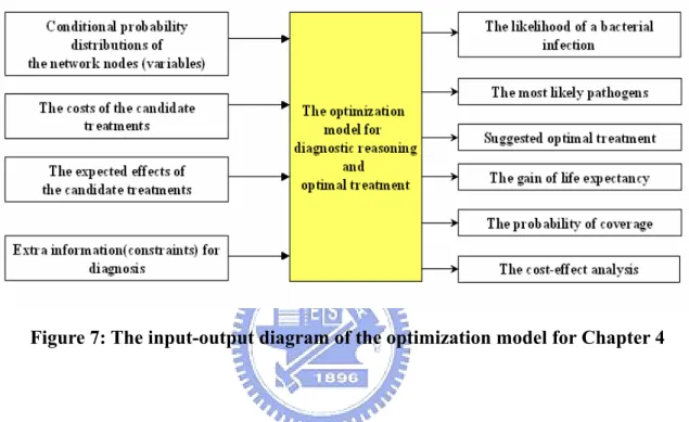
(51) 3.. Planning and diagnostic problems are not considered in one paradigm.. The limitations mentioned above restrict the practical usefulness of medical reasoning on Bayesian networks and influence diagrams in the following facts. First, the conditional probabilities between a node and its parent nodes could be fuzzy instead of a crisp numbers, owing to the difficulties of learning accurately the cause-effect relationships among the nodes. Second, as a common fact, the experts may have some professional speculations in the form of constraints between the nodes in a Bayesian network. These constraints could be boundary, dependency, or disjunctive conditions. Third, the investigators of influence diagrams used to maximize the utility functions by node removal processes [30,33,39] and ignore diagnostic reasoning tasks; on the other hand, Bayesian networks have been used widely in probabilistic reasoning but lacked the capability to suggest the optimal decision. This section proposes an optimization model to make diagnostic reasoning and treatment planning for bacterial infections, where the cause-effect relationships are expressed with an influence diagram and fuzzy data. The inputs of the reasoning system are conditional probability distributions of the network nodes, the associated costs of the candidate antibiotic treatments, the expected effects of the treatments, and extra constraints regarding belief propagation. Since the prevalence of the pathogens and infections are determined by many site-by-site factors and subjective knowledge, the decision may involve uncertainty not compliant with conventional approaches and quite different background. So we allow the decisions to be made under fuzzy environments, at which some of the parameters could be fuzzy parameters [7], and some constraints regarding diagnosis are introduced. When a patient is received, this reasoning system can, based on the present symptoms or bacteriological tests, help the clinician make precise diagnosis at the first decision point, and also supply the suggestions of optimal treatment for the infection.. The outputs of the. reasoning model are the likelihood of a bacterial infection, the most likely pathogen(s), the 41.