科技部補助專題研究計畫成果報告
期末報告
類別依變數模型中之內因自變數問題:方法論之探討與經濟投
票研究之應用(第2年)
計 畫 類 別 : 個別型計畫 計 畫 編 號 : MOST 104-2410-H-004-089-MY2 執 行 期 間 : 105年08月01日至106年10月31日 執 行 單 位 : 國立政治大學政治學系 計 畫 主 持 人 : 黃紀 計畫參與人員: 碩士級-專任助理:郭子靖 碩士班研究生-兼任助理:陳觀佑 碩士班研究生-兼任助理:張君憶 碩士班研究生-兼任助理:鄭琹尹 碩士班研究生-兼任助理:張世光 碩士班研究生-兼任助理:高舒 報 告 附 件 : 出席國際學術會議心得報告中 華 民 國 107 年 01 月 30 日
中 文 摘 要 : 政治學的經驗研究中,往往想估計並檢驗自變數對依變數的影響 ,而迴歸模型是最常應用的分析方法。如果該自變數為外因變數 (exogenous variable),符合條件獨立(conditional independence)的假定,則一般的迴歸分析便可估計不偏之係數。 不過棘手的是,若有其他未納入模型的變數同時影響到該自變數與 依變數,使該自變數與誤差項產生相關,便違反了條件獨立的假定 ,其迴歸係數估計值有「忽略變數偏差」(omitted variable bias),這類自變數常稱為「內因解釋變數」(endogenous explanatory variable)。例如經濟投票的學理,認為選民對經濟 的回顧或前瞻評估,會決定其投票的抉擇,獎勵或懲罰現任者及執 政黨。不過近年也有學者挑戰此一理論,認為選民的經濟評估其實 常受政黨認同的左右,偏袒自己喜歡的政黨,因此並非外因變數。 這類辯論因涉及變數在學理上的相對位置,其經驗檢證無法以單一 迴歸式中加入控制變數(control variables)來解決。儘管文獻中 對內因解釋變數的處理方式討論甚多,但大多是針對連續 (continuous)依變數,其中一般熟悉之「工具變數」
(instrumental variable, IV)及「兩階段最小平方法」(two-stage least square, 2SLS),並不宜套用至政治學中最常遭遇之 類別(categorical)依變數及其非線性迴歸模型。
有鑑於此,本兩年期研究計畫的目的有二:
一、 在方法方面:以廣義線性迴歸模型(generalized linear models, GLM)為基礎,結合中介分析(mediation analysis)與結 構方程式模型(structural equation model, SEM),發展適用於 類別依變數的內因解釋變數模型,不僅能一致估計迴歸係數,且能 正確解讀依變數的各類別發生的機率,避免非線性模型中「係數受 變異數尺度大小牽動」(coefficient- rescaling)引起之錯誤解 讀。 二、 在應用研究方面:將「類別依變數的內因解釋變數模型」應用 至經濟投票研究,既可克服傳統上將線性模型之IV 及2SLS 逕行套 用至類別依變數模型的問題,又可檢證學理上數種言之成理的觀點 論辯:例如選民的政黨認同是否先影響其回顧與前瞻經濟評估,然 後經濟評價才影響投票抉擇;還是經濟評估反映客觀的經濟榮枯 ,不會受政黨偏好的左右。 中 文 關 鍵 詞 : 內因解釋變數、類別依變數、廣義結構式模型、經濟投票、主權維 護
英 文 摘 要 : In empirical political studies, researchers often intend to estimate and test the effects of independent variables on dependent variables. Among various analysis methods, the regression model is the most commonly used one. If an
independent variable is an exogenous variable that fits the assumption of conditional independence, then the unbiased coefficients can be estimated with ordinary regression analysis. However, in cases where an independent variable and a dependent variable are simultaneously affected by other variables not included in the model, the independent variable will become correlated to the error terms. This
would violate the assumption of conditional independence, as the estimated value of its regression coefficient would contain "omitted variable bias." This type of independent variables is often called the "endogenous explanatory variable." In example, the economic voting theory suggests that voters' retrospective and prospective evaluations of the economy will determine their voting decisions, whether to reward or punish the incumbent and the ruling party. In recent years, however, some scholars have challenged this theory and argued that voters' economic evaluations are often affected by their party identifications. As voters tend to favor their preferred political party, their economic evaluation should not be considered as an
exogenous variable. This kind of debate involves variables' relative positions in theory, and its empirical analysis cannot be resolved by adding control variables to
regression model. Although the literature contains many studies on how to handle endogenous explanatory variables, they mostly target continuous dependent variables. Among these methods, the commonly noted "instrumental variables" (IV) and "two-stage least square" (2SLS) are not applicable to the categorical dependent variables and their nonlinear regression models that are most frequently encountered in politics. In view of the above arguments, this two-year research project has two objectives:
1. In terms of methods: This project will combine the basis of generalized linear models (GLM) with mediation analysis and structural equation model (SEM) to develop an
endogenous explanatory variable model that is applicable to categorical dependent variables. Not only will the model be able to consistently estimate the regression coefficient, but it can also correctly interpret the probability of occurrence for each category of dependent variables. This can avoid misinterpretations caused by
coefficient-rescaling in nonlinear models.
2. In terms of applied research: This project will apply the "categorical dependent variable's endogenous
explanatory variable model" to economic voting research. It will be able to solve the traditional problem of applying IV and 2SLS from linear models to categorical dependent variable models, as well as verify numerous plausible debates in theory. For example: do voters' party identifications influence their retrospective and prospective evaluations of the economy before their
economic evaluations affect the voting decisions, or do the economic evaluations reflect objective economic conditions independent of voters' party preferences.
英 文 關 鍵 詞 : endogenous explanatory variable, categorical dependent variable, generalized structural equation models, economic voting, Taiwan's sovereignty
1
壹、計畫背景及目的
政治學與社會科學的經驗研究中,往往想估計並檢驗自變數對依變數的影響,而迴歸模
型是最常應用的分析方法。如果該自變數為外因變數(exogenous variable)
,符合條件獨立(con-ditional independence)的假定,則一般的迴歸分析便可估計不偏之係數。不過棘手的是,若有 其他未納入模型的變數同時影響到該自變數與依變數,使該自變數與誤差項產生相關,便違
反了條件獨立的假定,其迴歸係數估計值有「忽略變數偏差」(omitted variable bias),這類自
變數常稱為「內因解釋變數」(endogenous explanatory variable)。例如經濟投票的學理,認為
選民對經濟的回顧或前瞻評估,會決定其投票的抉擇,獎勵或懲罰現任者及執政黨。不過近 年也有學者挑戰此一理論,認為選民的經濟評估其實常受政黨認同的左右,偏袒自己喜歡的 政黨,因此並非外因變數。這類辯論因涉及變數在學理上的相對位置,其經驗檢證無法以單 一迴歸式中加入控制變數(control variables)來解決。儘管文獻中對內因解釋變數的處理方式
討論甚多,但大多是針對連續(continuous)依變數,其中一般熟悉之「工具變數」(instrumental
variable, IV)及「兩階段最小平方法」(two-stage least square, 2SLS),並不宜套用至政治學中 最常遭遇之類別(categorical)依變數及其非線性迴歸模型。
有鑑於此,本兩年期研究計畫的目的有二:
一、 在方法方面:以廣義線性迴歸模型(generalized linear models, GLM)為基礎,結合中 介分析(mediation analysis)與結構方程式模型(structural equation model, SEM),發 展適用於類別依變數的內因解釋變數模型,不僅能一致估計迴歸係數,且能正確解讀 依變數的各類別發生的機率,避免非線性模型中係數受變異數尺度大小牽動 (coefficient- rescaling)引起之錯誤解讀。 二、 在應用研究方面:將「類別依變數的內因解釋變數模型」應用至經濟投票研究,既可 克服傳統上將線性模型之IV 及 2SLS 逕行套用至類別依變數模型的問題,又可檢證學 理上數種言之成理的觀點間之論辯:例如選民的政黨認同是否先影響其回顧與前瞻經 濟評估,然後經濟評價才影響投票抉擇;還是經濟評估反映客觀的經濟榮枯,不會受 政黨偏好的左右。 (一) 「內因解釋變數」分析方法之回顧 社會科學研究,常碰到感興趣的解釋變數有可能受到其他因素的影響,而被質疑為內因 自變數(Jackson 2008)。但文獻中對「內因性」(endogeneity)的指涉往往一詞多義,有時造 成辯論失焦。本研究計畫將釐清「內因」的來源,區分成「未觀測(潛在)因素」(unmeasured
confounder or latent factor)及「觀測到但模型中忽略的變數」兩大類,然後予以各個擊破。以 下先回顧文獻較豐富的線性模型處理方式,然後討論適合類別依變數的非線性模型(亦即廣 義之線性模型 generalized linear models, GLM,及其延伸)(參見 McCullagh and Nelder 1989; Hardin and Hilbe 2012; Agresti 2013; 黃紀、王德育 2016)中,內因問題的新挑戰,以利提出 本計畫對症下藥的思考方向。
1. 線性迴歸
適用連續依變數(continuous outcome variable)的線性模型,「內因」的首要來源,是未 觀測到的因素造成解釋變數與誤差項之間的相關,違反迴歸的條件獨立假定,使係數估計產
2
生偏誤。文獻中最常見的處理方式,一是找與內因自變數相關、但又不會直接影響依變數的 工具變數(instrumental variable, IV)來取代內因自變數(Angrist and Pischke 2009; Bollen 2012; Muller, Winship, and Morgan 2015; Sovey and Green 2011);另一個方法就是「兩階段最小平方
法」(two-stage least squares, 2SLS),以第一階段的輔助迴歸式估計內因自變數的預測值,然
後在第二階段將該預測值代入原來的結構迴歸式,利用預測值與結構是誤差項不相關的原理, 解決內因問題,Terza, Basu, and Rathouz(2008)也將 2SLS 稱為「兩階段預測值代入法」 (two-stage predictor substitution, 2SPS)。
政治學經驗研究中,在質疑模型中某個重要的解釋變數並非外因,而可能會受到其他觀
測到的變數的影響時,也稱該解釋變數為「內因變數」。例如Wlezien, Frank and Twiggs(1997)
等學者認為 Lewis-Beck(1988)等人之經濟投票理論中,選民之經濟評估其實是受到政黨認
同的影響,故選民對經濟表現好壞的評價,應是「內因」解釋變數。但幾乎所有的選舉相關 調查資料,都會測量受訪者的政黨偏好,故此一情況顯非未觀測的干擾因素造成,而是強調
該解釋變數學理的位置是「中介變數」(mediator, M):X 先影響 M,M 再影響 Y,而這正是
Baron and Kenny (1986)所倡導的「中介分析」(mediation analysis)。本計畫將此類解釋變數稱
為「內因中介變數」(endogenous mediator),其處理方式就是建立結構式模型(MacKinnon 2008;
Hayes 2013),而非 IV 或 2SLS。例如圖 1 中,若以 C 代表其他控制變數之向量,
X
C
M
Y
圖1 中介分析示意圖 則對應的結構式,由兩個迴歸式組成: 𝑀𝑖 = 𝛼1+ 𝛾1𝑋𝑖 + 𝑪𝑖𝜸2+ 𝜖1𝑖 𝑌𝑖 = 𝛼2 + 𝛽2𝑀𝑖 + 𝛾3𝑋𝑖 + 𝑪𝑖𝜸4+ 𝜖2𝑖 上式中,若兩式的誤差項沒有相關,則估計之係數解讀非常清楚,各司其職,例如𝛽̂2為M 對 Y 的影響,而𝛾̂1𝛽̂2可估計X 透過 M 對 Y 的間接效果。 2. 非線性迴歸 當M 或 Y 為類別變數時,迴歸式屬於非線性模型。這類模型在處理內因解釋變數時,比3
線性模型更為棘手。首先,由未觀測到之因素造成的內因問題,不能比照線性模型的 2SLS/2SPS 來處理。Terza, Basu, and Rathouz(2008)證明將 2SLS/2SPS 移植到 logit 或 probit 等非線性模型,則係數估計為偏誤。其次,近年隨著因果推論研究的發展,非線性模型的係
數估計值的解讀,受到重視。由於logit 或 probit 等非線性機率模型的誤差項變異數,因識別
(identification)的緣故,並未估計,因此係數估計值其實是真值 𝛽 除以標準差𝜎,但未估計 之𝜎不但在不同的迴歸式數值不同,且同一迴歸式也會隨著納入的自變數或控制變數不同而
異,故估計之係數難以做模型間之相互比較,稱之為「係數隨變異數尺度而異」
(coefficient-rescaling)問題(參見 Best and Wolf 2015; Breen and Karlson 2013; Breen, Karlson, and Holm 2013; Karlson, Holm, and Breen 2012; Winship and Mare 1984 等)。換言之,中介分析應用至非 線性迴歸構成的結構式模型,係數不宜直接解讀。因此本計畫在建立適用於類別依變數的內 因解釋變數模型時,也需兼顧估計值之正確解讀。 (二) 經濟投票研究中涉及內因問題的學理辯論 經濟投票理論認為選民會針對過去的經濟表現或未來的經濟展望,作為投票抉擇的主要 依據。文獻中依照時間面向區分為回顧型(retrospective)及前瞻型(prospective)經濟投 票,依照涵蓋層面區分為個人口袋型(pocket)及整體社會型(sociotropic)經濟投票。此一
理論在政治學中歷久不衰,尤其西方民主國家累積之文獻已卷帙浩繁(如Kanji and
Tan-nahill 2013; Lewis-Beck 1988; Lewis-Beck and Stegmaier 2007; Lewis-Beck, Nadeau, and Elias 2008; Lewis-Beck and Whitten 2013; Lewis-Beck, Nadeau, and Faucault 2013)。究其原因,一方 面因為經濟繁榮為普及價值(valence),幾無爭議可言,另一方面選民以在位者的經濟表現 為選舉投票之獎懲課責依據,邏輯也簡單明瞭。
不過近年來,學界浮現「修正學派」的挑戰聲浪,認為選民對經濟的評估並不客觀,多 半受到政黨認同的影響甚至扭曲(參見Anderson, Mendes, and Tverdova 2004; Duch 2008; Evens and Andersen 2006; Evens and Pickup 2010; Gerber and Huber 2010; Popescu 2013; Wlezien, Frank, and Twiggs 1997 等)。例如支持執政黨的選民傾向對經濟表現給正面評價, 而支持反對黨者則傾向給予負面評價。選民對經濟表現的判斷,受到其政黨色彩的影響,似 也不無道理。 經驗研究的重要功能之一,就在針對學理上的論辯蒐集資料,進行檢測。本研究計畫在 開發適用於類別依變數的內因解釋變數模型後,將應用於上述兩種經濟投票理論之分析。不 過應該強調的是:這兩個模型的檢測,無法以傳統的單一迴歸式加入控制變數來進行,因為 「修正派」的觀點,是認為選民的經濟評估扮演「中介者」M 的角色,受背後政黨認同 X 的影響,必須建立多個迴歸式的結構方程模型SEM 來檢測,以圖 1 為例,倘若 X 影響 M 的係數γ2在統計上不顯著,則表示M 為外因變數,對 Y 有其獨自的影響力,修正學派的觀 點未得到經驗數據的支持;反之,若γ2在統計上顯著且方向一如預期,則修正學派的觀點應 予正視。
Lewis-Beck and Stegmaier (2007, 532)在回顧經濟投票研究文獻時,發覺幾乎都是單一迴 歸式。台灣自民主化以來,經濟投票的研究也頗有進展(例如 黃秀端 1994;王柏燿 2004;盛杏湲 2009;吳親恩、林奕孜 2012;2013;Hsieh, Lacy, and Niou 1998; Choi 2010; Ho et al., 2013),不過分析方法亦以單一迴歸式為主。本研究計畫將此一主題之研究方法,
4
擴及適合類別變數的「廣義之結構式模型」(generalized SEM, GSEM)(Huang 2015)。
貳、執行進度與成果 本計畫第一年期自2015 年 8 月至今(2016 年 5 月),均依照規劃之進度執行,達成目標。 因應2016 年總統立委大選,除了分別在選前與選後展開電訪調查以蒐集個體資料之外,同時 也蒐集2016 年選舉結果如總統、立委的合格選民數、投票率、候選人與政黨得票率等總體資 料,以及有關總統立委選舉的新聞、剪報,政見發表會與辯論會錄影檔等質性資料。 一、 選民個體資料: 1. 電話訪問成果: 2016 年總統與立委選舉在 2016 年 1 月 16 日舉行,本計畫也在選前進行電話訪問,並在 選後針對選前獨立樣本進行追蹤,以取得研究資料。選前電訪期間自2015 年 11 月 23 日(星 期一)至11 月 29 日(星期日)由政大選舉研究中心執行,本次訪問預定完成 1,500 個樣本, 經實際執行後,獨立問卷共完成 1,515 個有效樣本,以 95%之信心水準估計,最大可能隨機 抽樣誤差為:±2.54%。為了追蹤選民實際投票結果,本計畫也在選後追蹤訪問選前完成的獨 立樣本;訪問期間自2016 年 1 月 24 日(星期日)至 1 月 28 日(星期四)由辦理選前電訪的 政大選研中心繼續執行,共完成843 個有效樣本。 2. 調查對象與抽樣方法: 本次電話訪問是以設籍在台灣地區且年滿20 歲以上的成年人為訪問對象。訪問樣本來自 選舉研究中心所累積的電訪資料庫,以隨機數修正電話號碼的最後四碼來製作電話樣本。在 開始訪問之前,訪員按照(洪式)戶中抽樣的原則,抽出應受訪的對象之後,再進行訪問。 3. 樣本代表性檢定: 為了瞭解1,515 份有效樣本的代表性如何,以下分別就性別、年齡、教育程度、戶籍地 等四方面予以檢定。 表1 訪問成功樣本之代表性檢定:性別(加權前) 樣 本 母 體 檢 定 結 果 人 數 百分比 百分比 男 722 47.7 49.4 卡方值=1.75830 p >0.05 樣本與母體一致 女 793 52.3 50.6 合 計 1,515 100 100.0
5 表2 訪問成功樣本之代表性檢定:年齡(加權前) 樣 本 母 體 檢 定 結 果 人 數 百分比 百分比 20─29 歲 170 11.4 17.2 卡方值=91.10108 p < 0.05 樣本與母體不一致 30─39 歲 252 16.8 21.2 40─49 歲 375 25.1 19.5 50─59 歲 371 24.8 19.2 60 歲以上 328 21.9 22.9 合 計 1,496 100.0 100.0 表3 訪問成功樣本之代表性檢定:教育程度(加權前) 樣 本 母 體 檢 定 結 果 人 數 百分比 百分比 小學及以下 123 8.2 15.5 卡方值= 120.14932 p< 0.05 樣本與母體不一致 國、初中 123 8.2 13.1 高中、職 450 29.9 28.2 專科 240 15.9 12.4 大學及以上 570 37.8 30.8 合 計 1,506 100.0 100.0 表4 訪問成功樣本之代表性檢定:戶籍地(加權前) 樣 本 母 體 檢 定 結 果 人 數 百分比 百分比 大臺北都會 290 19.2 21.8 卡方值=12.90951 p< 0.05 樣本與母體不一致 新北市基隆 116 7.7 8.8 桃竹苗 249 16.4 14.9 中彰投 310 20.5 19.1 雲嘉南 237 15.7 14.7 高屏澎 254 16.8 16.3 宜花東 58 3.8 4.4 合 計 1,514 100.0 100.0 由表1 至表 4 的樣本代表性檢定顯示:年齡、教育程度、及戶籍地樣本結構與母體並不 一致。為了使樣本與母體結構更符合,本研究對樣本的分布特性使用多變數「反覆加權法」 (raking)進行加權。 表5 至表 8 為加權後的樣本代表性檢定結果,顯示加權後的樣本結構和母體並無差異。
6 表5 訪問成功樣本之代表性檢定:性別(加權後) 樣 本 母 體 檢 定 結 果 人 數 百分比 百分比 男 743 49.0 49.4 卡方值= 0.06094 p > 0.05 樣本與母體一致 女 772 51.0 50.6 合 計 1,515 100.0 100.0 表6 訪問成功樣本之代表性檢定:年齡(加權後) 樣 本 母 體 檢 定 結 果 人 數 百分比 百分比 20─29 歲 255 3.9 17.2 卡方值= 0.04564 p > 0.05 樣本與母體一致 30─39 歲 316 21.2 21.2 40─49 歲 293 19.6 19.5 50─59 歲 286 19.1 19.2 60 歲以上 344 23.0 22.9 合 計 1,494 100.0 100.0 表7 訪問成功樣本之代表性檢定:教育程度(加權後) 樣 本 母 體 檢 定 結 果 人 數 百分比 百分比 小學及以下 233 15.5 15.5 卡方值= 0.65955 p> 0.05 樣本與母體一致 國、初中 189 12.5 13.1 高中、職 434 28.8 28.2 專科 183 12.1 12.4 大學及以上 468 31.1 30.8 合 計 1,507 100.0 100.0 表8 訪問成功樣本之代表性檢定:戶籍地(加權後) 樣 本 母 體 檢 定 結 果 人 數 百分比 百分比 大臺北都會 329 21.7 21.8 卡方值=0.00893 p> 0.05 樣本與母體一致 新北市基隆 134 8.8 8.8 桃竹苗 226 14.9 14.9 中彰投 290 19.1 19.1 雲嘉南 223 14.7 14.7 高屏澎 246 16.2 16.3 宜花東 67 4.4 4.4 合 計 1,515 100.0 100.0
7 本計畫已完成資料除錯,並建立 SPSS 統計軟體的電子檔,目前也已經使用本資料進行 初步分析,並撰寫研究論文至國際研討會發表。本計畫預計於執行結束後,連同編碼簿一同 繳送至「中央研究院調查研究專題中心資料庫」存查,未來對本電訪資料有興趣的研究人員, 可至該中心資料庫查詢相關細節並申請使用。 二、 集體資料: 1. 2016 年總統與立委選舉資料: 本計畫已完成 2016 年總統與立委選舉之集體資料之蒐集:除了中選會公布的各選舉類 型、各選區合格選民數、投票數、有效票數、無效票(廢票)數,以及各候選人、政黨的得票 數、得票率等資料之外,本計畫也同時計算並建置了以下有利於研究的加值資料,如:絕對 投票率(Vote shares of eligible electors)、有效政黨數(effective number of electoral parties, ENEP; effective number of parliamentary parties, ENPP)、有效候選人數(effective number of candidates)、 各選區候選人/政黨第二落選者與第一落選者得票數比率(Second-to-the-first loser ratio, SF Ratio)等。 依照不同選制劃分,蒐集的資料可區分為:總統、區域立法委員、山地與平地立法委員、 全國不分區立委政黨票等二項四類選舉之投票結果,統計單位分為縣市、鄉鎮市及行政區, 最小統計單位則細達村里,有助於統計分析的精確性及可比較性。 2. 2014 年 11 月九合一選舉至 2017 年 12 月底之地方選舉及補選資料: 除了九合一選舉為既定時程的定期改選,在選舉之後,有許多地區的地方公職人員,或 因涉及賄選、不法情事而遭法院判定當選無效後解職,或因辭職、病故等原因而需重新改選、 補選的情況,本計畫也依序蒐集相關的補選、重選等事由,以及各項補選結果。 上述資料均於蒐集、彙整、除錯完成後,存檔備查,並上傳至由本人長期建置並維護的 「台灣政治地緣資訊系統」(Taiwan’s Political Geography Information System, TPGIS,網址: http://tpgis.nccu.edu.tw/),對外開放給學術界研究人員及一般社會大眾查詢,以達善用學術資 源、成果共享的目標。 3. 台灣各類重要經濟指標、兩岸經貿互動狀況: 由於本計畫是以經濟投票為實證研究案例,因此也蒐集台灣自2000 年以來迄今的重要經 濟指標,以及兩岸經貿往來的發展狀況。蒐集的項目計有人口、土地、勞動力、國民生產與 所得、家戶所得與收支、消費與儲蓄、物價與景氣指數、進出口貿易額,以及兩岸投資、貿 易、往來國民人次等資料。詳細蒐集資料類型如附錄。 三、 其他質性資料: 本計畫除蒐集前述有關2016 年九合一選舉結果之總體、個體資料外,為使研究資料更加 充分,本計畫也蒐集本次選舉的相關中、英文新聞報導、文件、政府與選舉委員會公告等各 式資料共計將將近5.3 萬餘則(自 2015 年 8 月 1 日起,迄 2018 年 1 月 24 日止),其內容涵 蓋:(1)總統與立委選舉的官方期程、各項工作的舉辦時日等;(2)選舉方式(如社會上與 政府有針對總統與立委是否合併選舉、不在籍投票、電子投票、降低投票年齡與不分區政黨 票是否維持或降低分配立委席次門檻等等)、(3)不同選舉層級的競選策略(如各黨如何推派 適當的候選人、小黨又如何爭取選票)、(4)政黨互動(如競選前與競選期間大、小黨之間的
8 互動、合作與競爭)、(5)政黨與候選人之競選動態、(6)總統選舉對立委選舉的拉抬效應, 例如二位主要總統候選人蔡英文與朱立倫的競選熱烈程度如何拉抬民進黨與國民黨的立委競 選效果等、(7)針對各項選舉重要議題,例如馬習會、國民黨換柱案、王如玄軍宅案、蔡英 文家族炒作土地案、國、民兩黨與其他各政黨的總統與立委競選政見、族群認同與國家定位、 提振經濟與社會福利、重大改革議題如年金改革、司法改革、核能與能源政策、兩岸與美日 等外交經貿關係等新聞,以及民進黨政府上台後的各項重要政策、立院爭議議案、朝野與公 民社會對相關議題的看法、意見與重大爭議等質性資料,進行有系統地蒐集。將這些豐富的 參考資料分類、彙整歸檔後,預期將能充實研究內容,並有助於各項研究議題的發展,及提 升研究的效率。 參、分析結果: 本計畫結合「中介分析」與「結構方程式模型」,綜合而成適用於無序多分類(multinomial)
依變數之「廣義之結構方程式模型」(generalized structural equation model, GSEM,見頁 12 之 方程式(2)),並應用於前述蒐集之電訪追蹤資料。此一分析的結果,曾於 2017 年 10 月 20 日
在中研院社會所主辦的「公民與國家:台灣社會變遷基本調查第28 次研討會」中,以英文論
文 “Economic Voting: The Role of Partisanship and Mediation Analysis” 發表。該文具體描述了 本計畫資料之蒐集、模型建構、資料分析與研究發現,茲將主要之分析結果,呈現於下:
Modeling Strategy of Incorporating Partisan Effects
In terms of the question of how best to model economic voting, I recommend not to appeal to a tool kit of instrumental variable (IV) in such a haste. As Sovey and Green (2011) point out, good IV is not always available and requires careful justification. Instead, I advocate a theory-based modeling approach by casting the debates as competing models of the theoretical status of partisan-ship and economic perceptions. If the original economic voting paradigm is correct, then both par-tisanship and economic perceptions have only direct effects on voting choice. If the revisionist view is correct, than we need a separate equation to take account the mediation (or indirect) effect from partisanship to each economic perceptions and then from perceptions to voting decision. If neither of the separate equation finds significant effect of partisanship on economic perceptions, the revisionist view lacks empirical support and loses ground. But even if the effects of partisanship on economic perceptions are significant, the economic voting paradigm is not disconfirmed but only elaborated as a mediation mechanism. In any case, the key point here is that empirical test of the existence of mediation effect cannot be done in a single-equation format “followed by almost all practitioners in this field.” (Lewis-Beck andStegmaier2007, 532). This comment also applies to economic voting research on Taiwan since the island is known for its social cleavages and partisan divide (Huang 2017; Yu 2017). Structural equation modeling (see Kline 2016) is obviously a bet-ter albet-ternative, although it has to be generalized to accommodate both categorical mediators and
9
outcomes (Huang 2015).
An ideal way out of this endogeneity-exogeneity controversy is to use panel data with all the explanatory variables measured at time earlier than the outcome variable. However, panel data are relatively rare. Furthermore, not all panel data are equally applicable. As Gerber and Huber (2010) point out, the time difference between two waves of survey interview should be short enough to ensure no intervening events occur to “contaminate” the pre-election measurements. This type of pre- and post-election panel data conducted in a short time interval is even rarer. Postelection cross-sectional surveys are most available, but the measurement of retrospective eco-nomic assessment after election is often questioned as contaminated by respondent’s knowledge of who wins the election as well as the respondents’ voting choice (Wu and Lin 2012; 2013). This may be related to the recall type of questions for both voting behavior and retrospective perception in postelection surveys. Our two partisan effects hypotheses, once confirmed, also indicate the danger of contamination in post-election surveys of power-shifting elections. This is the case be-cause incumbent party and opposition party switch after power-shifting elections and so are the per-ceptions of their party identifiers.
A Generalized Structural Equation Model with Two Related Mediators
The central focus of the debate on the role of partisanship on economic perceptions is actually the theoretical status of the targeted explanatory variable, say M, in a causal system. That is, if X affects M and M in turn influences Y, then the effect of X on Y is (partially) mediated by M. I pre-fer calling such an explanatory variable a “mediator” so as to distinguish it from the confounding of latent variables discussed in the last section. Since X is observed, the best way to handle M is not just to question its exogeneity but to model X-M-Y relationships so as to test competing theories concerning M. This is exactly the subject of “mediation analysis” popularized by psychologists Baron and Kenny (1986).
Mediation analysis is widely used in the field of psychology and penetrated into social and bio-medical sciences (see, for example, MacKinnon 2008; Hayes 2013). It investigates the mecha-nisms that underlie an observed relationship between a primary independent variable and an out-come variable by examining how they relate to a third intermediate variable. Rather than hypothe-sizing only a direct causal relationship between the independent variable X and the dependent ble Y, a mediational model hypothesizes that the independent variable X affects the mediator varia-ble M, which in turn affects the outcome variavaria-ble Y. The simplest form of a mediation model is
10
often dubbed the “golden triangle.” The mediator M sitting on top of the triangle serves to illumi-nate the mechanisms through which X influences Y. It plays a pivotal role in understanding how the underlying process links X to Y and thus is no less, if not more, important than X. Therefore, the goal of mediation analysis goes beyond direct X-Y relationship by first testing the existence of X-M-Y relationship, and once established, estimating the extent to which the causal variable X in-fluences the outcome Y through one or more mediator variables M, called mediation (or indirect) effect. The effect of X on Y not mediated by M is called the direct effect.
When both the mediator and the outcome variables are continuous, standard mediation analysis is usually conducted in the regression-based path-analytic framework. In this setup, the standard method is to estimate the mediation effect using the product of coefficients of X and M. In nonlinear models such as binary, ordered or multinomial logit, comparing coefficients across equations is much more difficult. The challenges arise from the lack of separate identification of the mean and variance in these models. Although already shown in earlier literature (Maddala 1983; Winship and Mare 1984), this fact has often been overlooked until recent years when mediation and causal analyses are extended to nonlinear models (Breen and Karlson 2013; Breen, Karlson, and Holm 2013; Karlson, Holm, and Breen 2012). This “coefficient-rescaling” feature means that we cannot compare the coefficient of X from a logit or probit model excluding the mediator M with the corre-sponding coefficient from a logit or probit model including M. Likewise, multiplying coefficients from two different nonlinear equations makes little sense and cannot be interpreted as mediation ef-fect of X on Y transmitted through M. Instead, we should focused on the efef-fects on predicted probabilities of categories of the left-hand-side (LHS) variables (Imai, Keel, and Yamatomo 2010; Imai et al. 2011; Kuha and Goldthorpe 2010; Pearl 2012; Wooldridge 2010).
Based on Huang’s (2015) generalized SEM (GSEM) approach to tackle endogeneity in nonlin-ear models, I specify a three-equation model to examine economic voting in Taiwan’s 2016 presi-dential election. In this election, the lamb-duck incumbent was KMT President Ma Ying-jeou. The then-ruling KMT nominee was Allen Chu. The strong DPP candidate was Tsai Ing-wen. The third-party candidate was PFP’s James Soong.
The three-equation model addresses the endogeneity problems in two ways. First, all the ex-planatory variables are based on the first-wave pre-election panel survey (Huang 2016a), as sug-gested by Gerber and Huber (2010). Only the outcome variable Y of vote choice is from the post-election follow-up. Second, in order to take account of the endogeneity of subjective economic evaluations discussed earlier, I specify the sociotropic retrospective (M1) and prospective (M2)
11
and independents.1 Following Lockerbie’s (2008) argument, I allow the retrospective assessment
affect the prospective perception. The outcome variable (Y) of course is the voting choice among the three candidates. Our model specification can be illustrated as the diagram in Figure 1.
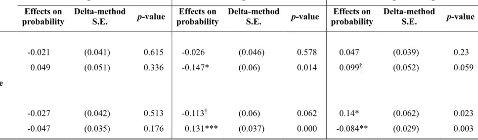
Data Source: Huang (2016).
Figure 1 Changes in Sociotropic Retrospective Economic Assessment as “Same or Better” before and after Presidential Election Day, Huang2016a pre- and post-election survevy
However, all the three left-hand-side variables are categorical variables, with both economic perceptions coded as 3-category (worse, the same, better) ordered variables while the outcome vari-able as 3-category nominal varivari-able (1=Chu, 2=Tsai, and 3=Soong). Appealing to the latent-varia-ble framework for ordinal varialatent-varia-bles, I assume the underlying propensity of choosing a particular category is continuous but unobserved. Our model can be formulated as a system of equations for latent LHS variables with superscripts “*”:
1 NP was not included in the GSEM model analysis because only 5 respondents in the panel sample identified them-selves with the New Party.
55.75 52.25 26.81 26.42 15.38 20 35.92 35.17 0 10 20 30 40 50 60 70 80 90 P ropor ti on of " the sa me or be tt er" (% ) Survey Wave KMT DPP NPP Non-partisans
12 (2) {
retrospective:
𝑀1𝑖∗ = 𝛾1𝑋𝑖+ 𝑪𝒊𝜸𝟐+ 𝑢1𝑖prospective:
𝑀2𝑖∗ = 𝛽1𝑀1𝑖∗ + 𝛾3𝑋𝑖+ 𝑪𝒊𝜸𝟒+ 𝑢2𝑖vote choice:
{ ln Pr(𝐶ℎ𝑢|𝑥) Pr(𝑆𝑜𝑜𝑛𝑔|𝑥)= 𝛽0,𝐶+ 𝛽2,𝐶𝑀1𝑖 ∗ + 𝛽 3,𝐶𝑀2𝑖∗ + 𝛾5,𝐶𝑋𝑖 + 𝑪𝒊𝜸𝟔,𝑪+ 𝑢3,𝐶 ln Pr(𝑇𝑠𝑎𝑖|𝑥) Pr(𝑆𝑜𝑜𝑛𝑔|𝑥)= 𝛽0,𝑇+ 𝛽2,𝑇𝑀1𝑖 ∗ + 𝛽 3,𝑇𝑀2𝑖∗ + 𝛾5,𝑇𝑋𝑖+ 𝑪𝒊𝜸𝟔,𝑻+ 𝑢3,𝑇where the vector C represents a vector of controlled covariates including social demographical vari-ables of gender, age, education, and attitude toward the fundamental cleavage issue of unification with China vs. Taiwan independence.
The relationship between each observed categorical and latent continuous variable is the famil-iar threshold model:
𝑀1 = { 1 if − ∞ ≤ 𝑀1𝑖∗ < 𝜏1,1 2 if 𝜏1,1 ≤ 𝑀1𝑖∗ < 𝜏1,2 3 if 𝜏1,2 ≤ 𝑀1𝑖∗ < ∞ 𝑀2 = { 1 if − ∞ ≤ 𝑀2𝑖∗ < 𝜏2,1 2 if 𝜏2,1 ≤ 𝑀2𝑖 ∗ < 𝜏2,2 3 if 𝜏2,2≤ 𝑀2𝑖∗ < ∞
In combination with the cumulative standard logistic distribution, the first two equations be-come familiar ordered logit, and the last is the multinomial logit.
Findings of Generalized SEM
Maximum likelihood (ML) estimates of our three-equation model (2)2 are listed in Tables 4 to
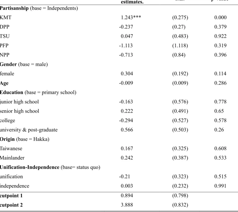
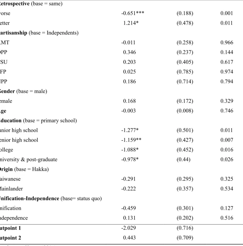
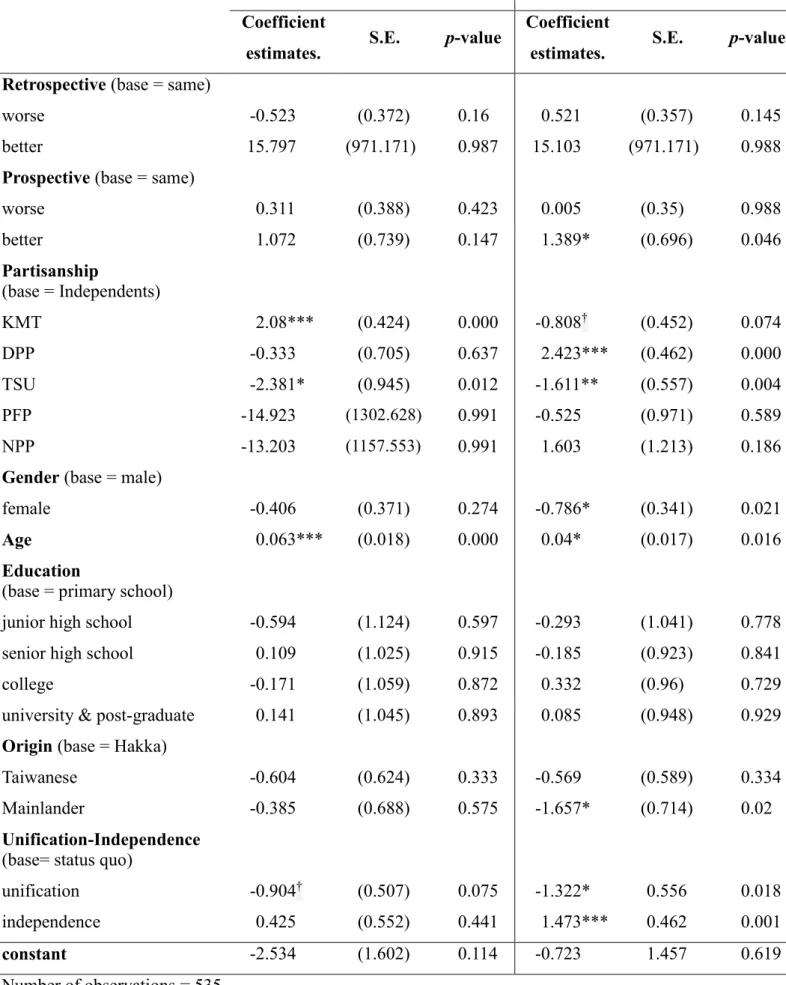
6. I first examine whether economic perceptions are exogenous variables or endogenous media-tors. As indicated in Table 4, retrospective economic assessment is affected by partisanship, with the then incumbent KMT identifiers tend to evaluate the past economic conditions more favorably than non-partisans. Next, Table 5 indicates that prospective economic assessment, though is not directly affected by partisanship, is affected indirectly through retrospective economic perception. This means that in Taiwan the partisan divide is deep and wide and it shapes both citizens’ evalua-tions of economy as well as presidential voting choice. Since this partisan divide has existed for more than two decades and constituted a long-term factor of citizens’ political attitudes and
13
ior, I conclude that in Taiwan if economic perceptions affect voting choice at all they tend to medi-ate the strong effects of partisanship.
[Tables 1 to 3 about here]
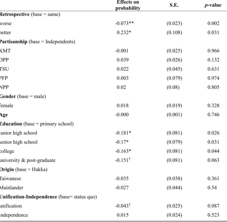
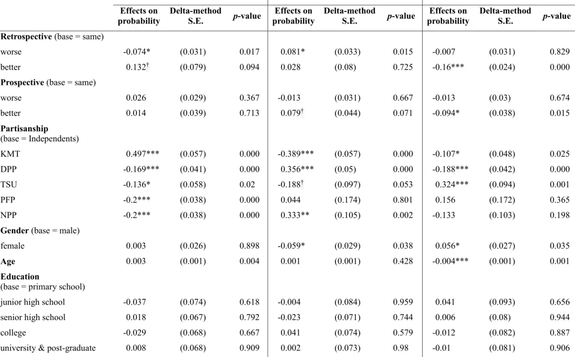
As explained in the last section, I use probability metric to evaluate and interpret the effects of explanatory variables in each equation on the LHS categorical variables. The two LHS variables in the first two equations are three-category (worse, the same, better) ordinal variables and rigor-ously speaking requires six tables with each contains “effects on probability” as well as standard er-rors estimated by delta-method (Green 2012) for each category. For the sake of parsimony, how-ever, I list only the effect on probability of choosing the highest category, i.e., perceiving the econ-omy has gotten better and will become better in Table 7 and Table 8, respectively. The final out-come variable of vote choice is multinomial and the effects of explanatory variables are listed in Ta-ble 9. Both TaTa-bles 7 and 8 indicate that in Taiwan the revisionist view is correct since partisanship significantly directly affects retrospective and indirectly affects prospective economic perceptions. For example, on average, KMT supporters are 0.053 more likely than non-partisans to believe the economy has gotten better over the past year. Furthermore, as shown in Table 8, optimistic/pessi-mistic retrospective assessment also tends to transmit to the prospective perception. After taking account partisan effects on economic perceptions, Table 9 indicates significant effects of retrospec-tive perceptions on voting choice as expected by the punishment-reward hypothesis of economic voting. On average those who consider the economy has gotten better have 0.132 higher probabil-ity of voting for the then incumbent KMT’s candidate Chu while those who consider economy has gotten worse have 0.072 lower probability of voting for Chu but 0.081 .higher probability of voting for the DDP’s Tsai. Curiously enough, positive prospective perception has weaker effect on vot-ing choice and is limited to favor the DPP’s Tsai against the PFP’s Soong. Overall, partisanship is indeed the most important determinant of vote choice, with economic voting tracing not far behind. Social and political cleavages, such as unification with China vs. Taiwan independence, are still sig-nificant but only on vote choices for Tsai and Soong, with voters leaning to Taiwan independence having 0.131 higher probability of voting for Tsai while those leaning toward unification having 0.14 higher probability of supporting Soong.
14
Table 1 Determinants of Retrospective Economic Perception
Coefficient
estimates. S.E. p-value
Partisanship (base = Independents)
KMT 1.243*** (0.275) 0.000
DPP -0.237 (0.27) 0.379
TSU 0.047 (0.483) 0.922
PFP -1.113 (1.118) 0.319
NPP -0.713 (0.84) 0.396
Gender (base = male)
female 0.304 (0.192) 0.114
Age -0.009 (0.009) 0.286
Education (base = primary school)
junior high school -0.163 (0.576) 0.778
senior high school 0.222 (0.491) 0.65
college -0.294 (0.527) 0.578
university & post-graduate 0.566 (0.503) 0.26
Origin (base = Hakka)
Taiwanese 0.167 (0.325) 0.608
Mainlander 0.242 (0.387) 0.533
Unification-Independence (base= status quo)
unification -0.21 (0.323) 0.515
independence 0.003 (0.232) 0.991
cutpoint 1 0.894 (0.798)
cutpoint 2 3.888 (0.832)
Data Source: Huang (2016).
15
Table 2 Determinants of Prospective Economic Perception
Coefficient
estimates. S.E. p-value
Retrospective (base = same)
worse -0.651*** (0.188) 0.001
better 1.214* (0.478) 0.011
Partisanship (base = Independents)
KMT -0.011 (0.258) 0.966
DPP 0.346 (0.237) 0.144
TSU 0.203 (0.405) 0.617
PFP 0.025 (0.785) 0.974
NPP 0.186 (0.714) 0.794
Gender (base = male)
female 0.168 (0.172) 0.329
Age -0.003 (0.008) 0.746
Education (base = primary school)
junior high school -1.277* (0.501) 0.011
senior high school -1.159** (0.427) 0.007
college -1.088* (0.452) 0.016
university & post-graduate -0.978* (0.44) 0.026
Origin (base = Hakka)
Taiwanese -0.291 (0.295) 0.325
Mainlander -0.222 (0.357) 0.534
Unification-Independence (base= status quo)
unification -0.459 (0.301) 0.127
independence 0.131 (0.202) 0.516
cutpoint 1 -2.029 (0.716)
cutpoint 2 0.443 (0.709)
Data Source: Huang (2016).
16
Table 3 Determinants of Presidential Voting Choice
Chu v. Soong Tsai v. Soong
Coefficient
estimates. S.E. p-value
Coefficient
estimates. S.E. p-value
Retrospective (base = same)
worse -0.523 (0.372) 0.16 0.521 (0.357) 0.145
better 15.797 (971.171) 0.987 15.103 (971.171) 0.988
Prospective (base = same)
worse 0.311 (0.388) 0.423 0.005 (0.35) 0.988 better 1.072 (0.739) 0.147 1.389* (0.696) 0.046 Partisanship (base = Independents) KMT 2.08*** (0.424) 0.000 -0.808† (0.452) 0.074 DPP -0.333 (0.705) 0.637 2.423*** (0.462) 0.000 TSU -2.381* (0.945) 0.012 -1.611** (0.557) 0.004 PFP -14.923 (1302.628) 0.991 -0.525 (0.971) 0.589 NPP -13.203 (1157.553) 0.991 1.603 (1.213) 0.186
Gender (base = male)
female -0.406 (0.371) 0.274 -0.786* (0.341) 0.021
Age 0.063*** (0.018) 0.000 0.04* (0.017) 0.016
Education
(base = primary school)
junior high school -0.594 (1.124) 0.597 -0.293 (1.041) 0.778
senior high school 0.109 (1.025) 0.915 -0.185 (0.923) 0.841
college -0.171 (1.059) 0.872 0.332 (0.96) 0.729
university & post-graduate 0.141 (1.045) 0.893 0.085 (0.948) 0.929
Origin (base = Hakka)
Taiwanese -0.604 (0.624) 0.333 -0.569 (0.589) 0.334
Mainlander -0.385 (0.688) 0.575 -1.657* (0.714) 0.02
Unification-Independence
(base= status quo)
unification -0.904† (0.507) 0.075 -1.322* 0.556 0.018
independence 0.425 (0.552) 0.441 1.473*** 0.462 0.001
constant -2.534 (1.602) 0.114 -0.723 1.457 0.619
Number of observations = 535 Log-likelihood = -1152.3834 Data Source: Huang (2016).
17
Table 4 Effects of Explanatory Variables on the Probability of Perceiving The State of the Economy Has Gotten “Better” over the Past Year
Effects on
probability S.E. p-value
Partisanship (base = Independents)
KMT 0.053*** (0.015) 0.001
DPP -0.005 (0.006) 0.405
TSU 0.001 (0.011) 0.923
PFP -0.016 (0.01) 0.133
NPP -0.012 (0.011) 0.275
Gender (base = male)
female 0.01 (0.007) 0.127
Age -0.000 (0.000) 0.299
Education (base = primary school)
junior high school -0.004 (0.015) 0.783
senior high school 0.007 (0.013) 0.626
college -0.007 (0.013) 0.611
university & post-graduate 0.02 (0.015) 0.19
Origin (base = Hakka)
Taiwanese 0.005 (0.01) 0.591
Mainlander 0.008 (0.013) 0.529
Unification-Independence (base= status quo)
unification -0.007 (0.01) 0.492
independence 0.000 (0.008) 0.991
Data Source: Huang (2016).
18
Table 5 Effects of Explanatory Variables on the Probability of Perceiving The State of the Economy Will Get “Better” in the Forthcoming Year
Effects on
probability S.E. p-value
Retrospective (base = same)
worse -0.073** (0.023) 0.002
better 0.232* (0.108) 0.031
Partisanship (base = Independents)
KMT -0.001 (0.025) 0.966
DPP 0.039 (0.026) 0.132
TSU 0.022 (0.045) 0.631
PFP 0.003 (0.079) 0.974
NPP 0.02 (0.08) 0.805
Gender (base = male)
female 0.018 (0.019) 0.328
Age -0.000 (0.001) 0.746
Education (base = primary school)
junior high school -0.181* (0.081) 0.026
senior high school -0.17* (0.079) 0.031
college -0.163* (0.081) 0.044
university & post-graduate -0.151† (0.081) 0.063
Origin (base = Hakka)
Taiwanese -0.035 (0.038) 0.361
Mainlander -0.027 (0.044) 0.54
Unification-Independence (base= status quo)
unification -0.043† (0.025) 0.087
independence 0.015 (0.024) 0.523
Data Source: Huang (2016).
19
Table 6 Effects of Explanatory Variables on the Probability of Voting for Chu, Tsai, and Soong
Voting for Chu Voting for Tsai Voting for Soong
Effects on probability Delta-method S.E. p-value Effects on probability Delta-method S.E. p-value Effects on probability Delta-method S.E. p-value
Retrospective (base = same)
worse -0.074* (0.031) 0.017 0.081* (0.033) 0.015 -0.007 (0.031) 0.829
better 0.132† (0.079) 0.094 0.028 (0.08) 0.725 -0.16*** (0.024) 0.000
Prospective (base = same)
worse 0.026 (0.029) 0.367 -0.013 (0.031) 0.667 -0.013 (0.03) 0.674 better 0.014 (0.039) 0.713 0.079† (0.044) 0.071 -0.094* (0.038) 0.015 Partisanship (base = Independents) KMT 0.497*** (0.057) 0.000 -0.389*** (0.057) 0.000 -0.107* (0.048) 0.025 DPP -0.169*** (0.041) 0.000 0.356*** (0.05) 0.000 -0.188*** (0.042) 0.000 TSU -0.136* (0.058) 0.02 -0.188† (0.097) 0.053 0.324*** (0.094) 0.001 PFP -0.2*** (0.038) 0.000 0.044 (0.174) 0.801 0.156 (0.172) 0.365 NPP -0.2*** (0.038) 0.000 0.333** (0.105) 0.002 -0.133 (0.103) 0.198
Gender (base = male)
female 0.003 (0.026) 0.898 -0.059* (0.029) 0.038 0.056* (0.027) 0.035
Age 0.003 (0.001) 0.004 0.001 (0.001) 0.428 -0.004*** (0.001) 0.001
Education
(base = primary school)
junior high school -0.037 (0.074) 0.618 -0.004 (0.084) 0.959 0.041 (0.093) 0.656
senior high school 0.018 (0.067) 0.792 -0.023 (0.071) 0.744 0.006 (0.08) 0.944
college -0.029 (0.068) 0.667 0.041 (0.074) 0.579 -0.012 (0.082) 0.887
university & post-graduate 0.008 (0.068) 0.909 0.002 (0.073) 0.98 -0.01 (0.081) 0.906
20
Table 6 Effects of Explanatory Variables on the Probability of Voting for Chu, Tsai, and Soong (Continued)
Voting for Chu Voting for Tsai Voting for Soong
Effects on probability Delta-method S.E. p-value Effects on probability Delta-method S.E. p-value Effects on probability Delta-method S.E. p-value
Origin (base = Hakka)
Taiwanese -0.021 (0.041) 0.615 -0.026 (0.046) 0.578 0.047 (0.039) 0.23
Mainlander 0.049 (0.051) 0.336 -0.147* (0.06) 0.014 0.099† (0.052) 0.059
Unification-Independence
(base= status quo)
unification -0.027 (0.042) 0.513 -0.113† (0.06) 0.062 0.14* (0.062) 0.023
independence -0.047 (0.035) 0.176 0.131*** (0.037) 0.000 -0.084** (0.029) 0.003
Data Source: Huang (2016).
21
肆、研究成果與發表論文狀況:
本計畫執行至今,已經將初步的研究成果撰寫五篇學術研討會論文,陸續發表於 2015、2016 及 2017 年的美國政治學年會(American Political Science Annual, APSA)國際學 術研討會、2015 年日本政治學年會,以及 2017 年的在中研院社會所主辦的「公民與國家: 台灣社會變遷基本調查第28 次」研討會。APSA 年會是全美政治學界最大、同時也是最知 名的國際學術研討會,有許多國際政治學與社會科學界知名學者與頂尖研究人員參與。本人 親自參與三次年會,並於會中宣讀論文。 每次參與學術研討會議時,本人除發表研究成果及會議論文之外,也由參與會議的學者 們進行問答、解釋,在彼此討論的同時,每每獲得許多寶貴的建議,有助進一步修改並精緻 化研究論文後投稿至專業學術期刊發表,並使本研究的執行過程與成果更為順利、完整。 本計畫執行至今所發表的五篇學術研討會論文的研究重點及成果詳述於下:
1. Huang, Chi, and Kah-Yew Lim. 2015. "Voter Turnout in Concurrent Elections: Does the Number of Ballots Matter?" Paper presented at the 2015 Annual Meeting of the American Political Science Association. San Francisco, CA. September 2-5, 2015.
受惠於本計畫補助出席國際學術研討會之經費,本人已將部分研究成果發表於2015 年
美國政治學年會(American Political Science Annual, APSA)國際學術研討會。APSA 年會是 全美政治學界最大、同時也是最知名的國際學術研討會,有許多國際政治學與社會科學界知
名學者與頂尖研究人員參與。本次會議是在2015 年 9 月 4 日至 9 月 7 日,於美國加州的舊
金山市舉辦。本人於會議的第一天(9 月 4 日),即在「台灣民主政治、投票與公共意見」 (Taiwan's Domestic Politics, Voting, and Mass Opinion)的討論組中,將本計畫蒐集的集體資 料,與本計畫延攬的博士後研究員林啟耀合作撰寫成研究論文,並在會中發表。本研究論文 係以2014 年我國九合一地方公職人員合併選舉為例,探討多項選舉在同時舉行的狀況下, 針對拿到不同公職人員選票張數的直轄市非原住民選區選民(三張選票:市長、市議員、里 長)與直轄市原住民選區選民(五張選票:市長、市議員、里長,另有原住民自治區長、原 住民自治區代表)的投票率進行比較。研究結果發現,與某一類型的選舉合併舉行時,對提 升其他類型選舉的投票率,有明顯的影響。
2. Lim, Kah-Yew, Chi Huang, and Ching-hsin Yu. 2016. "Assessment of Cross-strait Policy and Voting Choices in Taiwan's 2016 Presidential Election." Paper presented at the 2016 Annual Meet-ing of the Japanese Association of Electoral Studies. Tokyo: Nihon University. May 14-15, 2016.
在完成 2016 年總統與立委大選前後的二波電話訪問後,本研究也嘗試將蒐集到的個體 量化資料進行初步分析,並與本計畫延攬博士後研究員林啟耀、政大選舉研究中心游清鑫研 究員一同撰寫學術論文,發表於 2016 年日本選舉協會(Japanese Association of Electoral Studies, JAES)年會中。本論文主要聚焦於兩岸經貿利益與國家主權之間的權衡與影響,經 濟效益雖然有助於執政者,但未適當維護主權卻不利於現任政府爭取連任。研究結果顯示, 與以往的研究相仿,經濟利益是選民的重要考量因素,對於兩岸經貿互動有正面評價的選民 更有可能支持現任的國民黨總統候選人;2012 年總統大選的結果證實馬政府因為兩岸經貿 互動的經濟表現而獲得選民支持。然而在 2016 年的選舉中,維護主權的問題比經濟表現產 生了更大的影響,選民在選擇投票對象時,也一併將主權面臨的迫切問題列入考量。
22
3. Huang, Chi, and Kah-Yew Lim. 2016. "Coattail and Reverse Coattail Effects: The Case of Tai-wan's 2016 Election." Paper presented at the 2016 Annual Meeting of the American Political Sci-ence Association. Philadelphia, September 1-4, 2016.
為了讓 2016 年總統與立委大選前後蒐集的質性與總體資料發揮效益,本計畫嘗試對這 些重要資料展開分析,並與本計畫延攬博士後研究員林啟耀一同撰寫學術論文,並於 2016 年 APSA 國際學術研討會上發表。本次會議是在 2016 年 9 月 1 日至 4 日於美國費城舉辦, 本論文的重點是研究台灣 2016 年同時舉行的總統和立委大選,此個案的獨特性在於國民黨 的總統候選人朱立倫同時存在正向與反向的總統拉抬效果。依照理論,參選政黨為了同時在 總統與立委席次上獲得勝選,政黨提名的總統候選人應該會儘可能發揮對同黨立委候選人的 拉抬效果;然而對於缺乏高知名度和個人魅力的總統候選人來說,裙帶效應可能因不同立委 選區的競選狀態而異。意即,總統選舉的拉抬效果可能只存在於實力較弱、或是初次投入選 戰的立委候選人,而不存在於競選連任的現任立委;而後者更有可能出現反向的拉抬效果。 本文先透過非遞歸模型來估計選區的總體得票資料。結果顯示,在民進黨方面,蔡英文 對同黨立委具有正向的拉抬效果;但國民黨方面則既沒有正向、也沒有反向的拉抬效果出 現。另一方面,以雙變量機率單元模型(bivariate probit models)分析 TEDS2016 電訪的個 體資料後,發現只有在受訪者對總統候選人評價較高的時候,才會出現對同黨立委候選人的 拉抬效果。進一步分析總統候選人實際得票與立委得票的影響時,國民黨陣營出現了明顯的 反向拉抬效應。透過總體與個體訪問調查資料的分析,分別顯示出候選人形象與實際投票選 擇的差異。最後,本文的分析結果顯示,個人層次的調查資料可能比總體更適合用於分析總 統選舉的拉抬效應。
4. Huang, Chi, Kah-Yew Lim, Lu-huei Chen, and Eric Chen-hua Yu. 2017. “The Emergence of New Parties: A Case Study of the New Power Party in Taiwan.” Paper presented at the 2017 Annual Meeting of the American Political Science Association. San Francisco, CA. August 31-September 3, 2017.
本文的重點是2016 年選舉中新政黨:時代力量的崛起,並分別從環境機會
(environmental opportunity),創造新議題(demand side of new issues),獲得民眾普遍支持 的政黨領袖(populist leaders)的出現、以及選舉制度的激勵和約束(institutional incentives and constraints of electoral systems)等理論角度來分析此一個案,同時結合質性資料以追蹤 關鍵事件,並透過量化方法分析個體訪問結果和選區總體選舉資料。我們發現,時代力量政 黨領袖們一方面以呼籲年輕一代來發動社會運動,另一方面也證明時代力量是取代台灣團結 聯盟的可行選擇;後者雖然在立院具有席次,然而卻相對缺乏選舉競爭力。最終,時代力量
成功贏得超過5%政黨票的門檻並獲得不分區立委的席次。同樣重要的是,時代力量瞄準了
國民黨的失政議題,並在部分選區成功獲得選前在野的民進黨的禮讓。
5. Huang, Chi. 2017. "Economic Voting: The Role of Partisanship and Mediation Analysis." Pre-sented at the 28th Conference on the Taiwan Social Change Survey. Taipei: Institute of Sociology, Academia Sinica. October 20, 2017.
23 討會中的研究論文。在評價過去經濟表現和未來前景,以研究選舉問責制的議題上,經濟投 票模型已經成為研究典範。然而,最近的對於經濟投票的「修正主義觀點」認為:經濟投票 是「內生性」的,因為對於特定政黨的支持強烈,影響了選民對總體經濟表現的看法。過往 研究對這種「政黨偏見」主張有不同的看法,但很少直接分析政黨偏見是否影響經濟認知並 探討其因果效應。 本文試圖以因果推論的方式,結合以競爭模型為基礎的中介分析(competing-models-based mediation analysis)。研究策略是同時利用本計畫在 2016 年台灣總統大選選前所執行的 電話訪問及選後追蹤調查所建立定群追蹤資料,並搭配其他重複橫斷面調查(repeated cross-sectional surveys, RCS)資料來分析此議題。同時,本研究在理論和方法論的方面尋求突 破,除了採用準實驗設計(quasi-experimental design)分析政黨效應的潛在結果,透過差分 法(differences-in-differences method)驗證政黨對經濟評價的影響、估計影響效果之外,也 改善過往文獻中只利用傳統單一方程式的方式,提出中介分析方法並建立一般結構方程模型 (generalized structural equation models, GSEM)來分析政黨偏見、經濟評價和投票選擇之間 的因果關係。 伍、結論與建議: 一、結論: 本計畫在執行期間,已在台灣、美國、日本等地舉行的國際專業學術研討會中發表五篇 研究論文,同時也陸續完成重要的個體、總體與量化、質性研究資料的蒐集與彙整。這些寶 貴的資料及執行成果順利達成整體計畫原先規劃的目標。 二、建議: 本計畫在執行過程中與實際分析時發現,要分析選舉結果造成政黨輪替時的案例中,選 民如何在經濟評價與經濟投票抉擇上出現變化,非常需要透過選前訪問與選後追蹤所建立起 來的定群追蹤資料來分析;可惜的是,國內學界往往侷限於研究經費、人力等相關資源,而 難以執行追蹤調查,也不易建立用以分析、研究的定群追蹤資料。本計畫在此強烈建議貴部 往後可以繼續補助試圖建立追蹤調查的研究計畫案,為研究者提供必要且充分的研究資源, 以利取得調查與研究結果。 伍、參考文獻 王柏燿,2004,〈經濟評估投票抉擇:以 2001 年立法委員選舉為例〉,《選舉研究》,11(1): 171-195。 吳親恩、林奕孜,2012,〈經濟投票與總統選舉:效度與內生問題的分析〉,《台灣政治學 刊》,16(2): 175-232。 吳親恩、林奕孜,2013,〈兩岸經貿開放、認同與投票選擇:2008 年與 2012 年總統選舉的分 析〉,《選舉研究》,20(2): 1-36。 黃秀端,1994,〈經濟情況與選民投票抉擇〉,《東吳政治學報》,3: 97-123。 黃紀、王德育,2016,《質變數與受限依變數的迴歸分析》,臺北:五南。 Agresti, Alan. 2013. Categorical Data Analysis. 3rd edition. New Jersey: Wiley.
24
Voting: Evidence from the 1997 British Election.” Electoral Studies 23(4): 683-708.
Angrist, Joshua D. and Jörn-Steffen Pischke. 2009. Mostly Harmless Econometrics: An Empiricist’s Companion. Princeton: Princeton University Press.
Baron, Reuben M., and David A. Kenny. 1986. “The Moderator-Mediator Variable Distinction in Social Psychological Research: Conceptual, Strategic, and Statistical Considerations.” Jour-nal of PersoJour-nality and Social Psychology 51(6): 1173-1182.
Best, Henning, and Christof Wolf. 2015. “Logistic Regression.” In The SAGE Handbook of Regres-sion Analysis and Causal Inference, ed. Henning Best and Christof Wolf. London: Sage. Bollen, Kenneth A. 2012. “Instrumental Variables in Sociology and the Social Sciences.” Annual
Review of Sociology 38: 37-72.
Breen, Richard, and Kristian Bernt Karlson. 2013. “Counterfactual Causal Analysis and Nonlinear Probability Models.” In Handbook of Causal Analysis for Social Research, ed. Stephen L. Morgan. Heidelberg: Springer.
Breen, Richard, Kristian Bernt Karlson, and Anders Holm. 2013. “Total, Direct, and Indirect Effects in Logit and Probit Models.” Sociological Methods & Research 42(2): 164-191.
Choi, Eunjung. 2010. "Economic Voting in Taiwan: The Significance of Education and Lifetime Economic Experiences." Asian Survey 50(5): 990-1010.
Duch, Raymond M., and Randolph T. Stevenson. 2008. The Economic Vote: How Political and Eco-nomic Institutions Condition Election Results. Cambridge: Cambridge University Press. Evans, Geoffrey, and Mark Pickup. 2010. “Reversing the Causal Arrow: The Political Conditioning
of Economic Perceptions in the 2000–2004 U.S. Presidential Election Cycle.” The Journal of Politics 72(4):1236-1251.
Evans, Geoffrey, and Robert Andersen. 2006. “The Political Conditioning of Economic Perceptions.” The Journal of Politics 68(1):194-207.
Gerber, Alan S., and Gregory A. Huber. 2010. “Partisanship, Political Control, and Economic As-sessments.” American Journal of Political Science 54(1): 153-173.
Hardin, James W., and Joseph M. Hilbe. 2012. Generalized Linear Models and Extensions. 3rd edi-tion. Texas: Stata Press.
Hayes, Andrew F. 2013. Introduction to Mediation, Moderation, and Conditional Process Analysis: A Regression-Based Approach. New York: The Guilford Press.
Ho, Karl, Harold D. Clarke, Li-Khan Chen, and Dennis Lu-Chung Weng. 2013. "Valence Politics and Electoral Choice in a New Democracy: The Case of Taiwan." Electoral Studies 32(3): 476-481.
Hsieh, John Fuh-Sheng, Dean Lacy, and Emerson M.S. Niou. 1998. “Retrospective and Prospective Voting in a One-Party-Dominant Democracy: Taiwan's 1996 Presidential Election.” Public Choice 97(3): 383-399.
Huang, Chi. 2015. “Endogenous Regressors in Nonlinear Probability Models: A Generalized Struc-tural Equations Modeling Approach.” Journal of Electoral Studies 《選舉研究》,22(1): 1-33.
25
Huang, Chi. 2016. "Endogenous Explanatory Variables in Models with Categorical Outcome: Inno-vative Methods and Applications to Economic Voting Research." [In Chinese] MOST 104-2410-H-004-089-MY2. Taipei: Ministry of Science and Technology Research Project (First-Year Report)
Huang, Chi. 2017. “Electoral System Change and Its Effects on the Party System in Taiwan.” In The Taiwan Voter, ed. Christopher H. Achen and T.Y. Wang. Ann Arbor: University of Michigan Press.
Jackson, John E. 2008. “Endogeneity and Structural Equation Estimation in Political Science.” In The Oxford Handbook of Political Methodology, eds. Janet Box-Steffensmeier, Henry E. Brady, and David Collier. Oxford: Oxford University Press, pp. 404-431.
Karlson, Kristian Bernt, Anders Holm, and Richard Breen. 2012. “Comparing Regression Coeffi-cients Between Same-Sample Nested Models Using Logit and Probit: A New Method.” Soci-ological Methodology 42(1): 286-313.
Kline, Rex B. 2016. Principles and Practice of Structural Equation Modeling, 4th edition. New York:
The Guilford Press.
Lewis-Beck, Michael S. 1988. Economics and Elections: The Major Western Democracies. Ann Ar-bor: University of Michigan Press.
Lewis-Beck, Michael S., and Marina Costa Lobo. 2017. "The Economic Vote: Ordinary vs. Extraor-dinary Times." In The SAGE Handbook of Electoral Behaviour. Vol. 2, ed. Kai Arzheimer, Jocelyn Evans and Michael S. Lewis-Beck. London: SAGE.
Lewis-Beck, Michael S., and Guy D. Whitten. 2013. “Economics and Elections: Effects Deep and Wide.” Electoral Studies 32(3): 393-395.
Lewis-Beck, Michael S., and Mary Stegmaier. 2007. "Economic Models of Voting." In The Oxford Handbook of Political Behavior, eds. Russell J. Dalton and Hans-Dieter Klingemann. Oxford: Oxford University Press.
Lewis-Beck, Michael S., Richard Nadeau, and Angelo Elias. 2008. “Economics, Party, and the Vote: Causality Issues and Panel Data.” American Journal of Political Science 52(1): 84-95. Lewis-Beck, Michael S., Richard Nadeau, and Martial Foucault. 2013. “The Compleat Economic
Voter: New Theory and British Evidence.” British Journal of Political Science 43(2): 241-61. MacKinnon, David P. 2008. Introduction to Statistical Mediation Analysis. New York: Lawrence
Erlbaum Associates.
McCullagh, P. and J.A. Nelder. 1989. Generalized Linear Models, 2nd edition. London, Chapman and Hall.
Muller, Christopher, Christopher Winship, and Stephan L. Morgan. 2015. “Instrumental Variables Regression.” In The SAGE Handbook of Regression Analysis and Causal Inference, ed. Hen-ning Best and Christof Wolf. London: Sage.
Popescu, Gheorghe H. 2013. “Partisan Differences in Evaluations of the Economy.” Economics, Management and Financial Markets 8(1): 130-135.
Sovey, Allison J., and Donald P. Green. 2011. “Instrumental Variables Estimation in Political Sci-ence: A Readers’ Guide.” American Journal of Political Science 55(1): 188-200.
26
Terza, Joseph V.,Anirban Basu, and Paul J. Rathouz. 2008. “Two-Stage Residual Inclusion Estima-tion: Addressing Endogeneity in Health Econometric Modeling.” Journal of Health Econom-ics 27(3): 531-543.
Winship, Christopher, and Robert D. Mare. 1984. “Regression Models with Ordinal Variables.” American Sociological Review 49(4): 512-525.
Wlezien, Christopher, Mark Franklin, and Daniel Twiggs. 1997. “Economic Perceptions and Vote Choice: Disentangling the Endogeneity.” Political Behavior 19(1): 7-17.
Yu, Ching-hsin. 2017 “Parties, Partisans, and Independents in Taiwan.” In The Taiwan Voter, ed. Christopher H. Achen and T.Y. Wang. Ann Arbor: University of Michigan Press.
27 附錄:本計畫蒐集之經濟指標資料類目(2000-2017) 項次 項目 週期* 範圍 1 人口:年齡、年齡結構*、性別比例 Y 鄉鎮 2 土地:公有、私有土地面積 Y 鄉鎮 3 土地:家戶每人平均居住面積 Y 縣市 4 經濟成長率** Y/Q 全國 5 國內生產毛額(GDP)與產業結構* Q 全國
6 國民所得(NI)、平均 per capita NI Q 全國
7 消費:民間支出、政府支出、資本形成 Y 全國 8 儲蓄:國內儲蓄毛額 Y 全國 9 貿易:對主要國家進口、出口額 Y 全國 10 勞動:就業人數與行業結構、失業人口數、失業率 Y 縣市 11 工商及服務業受雇人口數、每人每月平均薪資 M 全國 12 家庭平均收支 Y 縣市 13 台灣對中國投資、中國對台灣投資申請件數 M 全國 14 台灣對中國投資、中國對台灣投資金額統計 M 全國 15 消費者物價指數CPI M 全國 16 景氣指標及燈號 M 全國 資料來源: 1. 「主要經濟指標統計報表」(行政院主計總處) 2. 《中華民國統計年鑑》(內政部) 3. 《各縣市統計要覽》(各縣市政府) 4. 陸委會《兩岸經濟統計月報、經濟部投審會《核准僑外投資、陸資來臺投資、國外投資、 對中國大陸投資統計月報》、主計總處《物價統計月報》 5. 國家發展委員會「景氣指標查詢系統」。 *說明: 1. 統計週期縮寫表說明: 1) Y:年度 2) HY:半年度 3) Q:季度 4) M:月份 2. 年齡結構分為 0-15 歲(預備勞動力)、16-64 歲(勞動力)、65 歲以上(退休) 3. 產業結構分為初級產業(農林漁牧)、二級產業(工業)、三級產業(商業與服務業)。 4. **經濟成長率雖然有季度資料,但它是「年增率」,也就是某年Qi 季相對於去年的 Qi 季 的年增長率。如果是要算每季的成長率,則需要按照每季與上一季的資料自行計算。 5. 此外致電詢問經濟部投資業務處有關台商人數、設廠數與台籍人士在陸就業人數,投資處 表示因為「台商」身分難以認定,因此沒有做相關統計。