資產報酬率波動度不對稱性與動態資產配置 - 政大學術集成

全文

(1)國立政治大學金融研究所博士論文指導教授：廖四郎博士. . y. sit er. al. n. . io. . Nat. . ‧. . 學. . 政治大資產報酬率波動度不對稱性與動態資產配置立. ‧ 國. . Ch. engchi. i Un. v. 研究生：陳正暉中華民國九十九年四月 .

(2) . Asymmetric Volatility in Asset Returns and Dynamic Asset Allocation. 立. 政治大. ‧. ‧ 國. 學. n. er. io. sit. y. Nat. al. Ch. engchi. I . i Un. v.

(3) ABSTRACT This study significantly extends the applicability of time-changed Lévy processes to the portfolio optimization. The leverage effect directly induces the intertemporal asymmetric volatility hedging demand, while the volatility feedback effect exerts a minor influence via the leverage effect. under. the. pure-continuous. time-changed. Lévy. process.. Furthermore, the leverage effect still plays a major role while the volatility feedback effect just works over the short-term investment. 政治大. horizon under the infinite-jump Lévy process. Based on the proposed. 立. general stochastic asymmetric volatility asset return model, we conclude. ‧ 國. 學. that the diffusion term is an essential determinant of financial modeling for index dynamics given infinite-activity jump structure.. ‧. n. er. io. sit. y. Nat. al. Ch. engchi. II . i Un. v.

(4) Contents 1. Introduction. 1. 2. Time-Changed Lévy Processes with Asymmetric Volatility. 8. 2.1. Fundamental Properties of Lévy Process. 8. 2.2. Stochastic Time Changes for Lévy Processes. 10. 2.3. Time-Changed Asset Price Processes with Asymmetric Volatility. 12. 政治大 2.3.1 Pure-Continuous Asset Dynamic Process 立 2.3.2 Infinite-jump Asset Dynamic Process. 14 16. ‧ 國. 學. 3. Dynamic Asset Allocation. 23. Investment Opportunity Set and Investor Preference. 23. 3.2. Pure-Continuous Asset Dynamic Process. 25. ‧. 3.1. sit. y. Nat. io. Infinite-Jump Asset Dynamic Process. al. n. 3.3. Ch. er. 3.2.1 Numerical Examples. n engchi U. 3.3.1 Reduced Time-Changed Lévy Process. iv. 3.3.2 Numerical Examples. 28 34 39 42. 4. Empirical Results. 48. 4.1. The General Stochastic Asymmetric Volatility Model. 48. 4.2. Data and Model Parameter Estimation. 50. 5. Concluding Remarks. 60. References. 63. Appendices. 69. III .

(5) Chapter 1 Introduction. CHAPTER 1. Introduction Merton (1971) carried out seminal work on intertemporal optimal portfolio choices assuming a Gaussian distribution in asset returns. Following the framework of Merton, diffusion has been. 治政大uncertainty with regard to investthe standard continuous-time stochastic process representing 立 ment opportunities for optimizing portfolio choice.. ‧ 國. 學. The focus of asset price modeling has shifted to a framework based on non-Gaussian distribu-. ‧. tion to alleviate problems in underestimating the frequency and magnitude of extreme events,. sit. y. Nat. namely, crashes and booms. Particularly, many early empirical evidences have fundamentally. io. al. er. shaken assumptions made by the diffusion model, for instance, Mandelbrot (1963), Fama (1965). iv n C h e n gflux. Portfolio optimization is a field in continuous i U returns are non-Gaussian, the Merc hWhen n. and Engle (1982). Recently, Jondeau et al. (2007) published an organized treatise on this topic.. ton rule may fail to optimize a portfolio due to the first and second moments are no longer fully representing asset return specifications in real financial markets. Furthermore, advanced improvement in financial modeling provides researchers and participants with insights into portfolio optimization, asset pricing, and risk management. Particularly, observations of real asset markets reveal numerous stylized facts. Cont (2001) comprehensively summarized the facts, such as asymmetric volatility, aggregated normality, and absence of serial correlation, etc.. -1-.

(6) Chapter 1 Introduction. Among these non-Gaussian specifications, asymmetric volatility and fat tail are relevant considerations with regard to asset allocation decisions (see Chunhachinda et al. (1997)). Campbell et al. (1997, Chapter 12) explained asymmetric volatility in terms of the leverage and volatility feedback effects. The leverage effect proposed by Black (1976), Christie (1982) and Nelson (1991), claimed that a negative equity return reduces the leverage firm value and thus increases the risk of holding equity, thus increasing volatility risk. Additionally, the volatility feedback effect proposed by Campbell and Hentschel (1992), Bekaert and Wu (2000) and Wu (2001) ad-. 政治大. vocated that it should be satisfied if return volatility behavior involves persistent clustering, in. 立. which case a shock in either direction enhances the anticipated increase in volatility and increase. ‧ 國. 學. the required rate of return for holding stocks, and furthermore, reduces the asset price to enable. ‧. higher future returns. Kraus and Litzenberger (1976) demonstrated that investors with the power utility favor positive over negative skewness. Therefore, the leverage and volatility feedback. y. Nat. er. io. sit. effects significantly influence optimal portfolio choices when asset return has asymmetric volatility. While asymmetric volatility is of central interest in the context of portfolio optimization,. n. al. Ch. i Un. v. the area is under-researched and comparatively neglected, particularly for continuous-time asset return models.. engchi. The Lévy process has recently been applied to asset price modeling in response to such criticisms. Since Lévy processes offer the merit of extending the scope of the distribution via the law of infinite divisibility and/or independent increment property, the price change can be expressed as the result of the aggregation of random economic shocks. Moreover, non-Gaussian or discontinuous specifications for stylized facts are characterized by Lévy measure (density) which de-. -2-.

(7) Chapter 1 Introduction. scribes the arrival rate for jumps of all sizes. The finance literature has extensively explored the setting of Lévy density, for instance, Variance Gamma (VG) was presented by Madan and Seneta (1990) and extended to skewness by Madan et al. (1998), CGMY was adapted by Geman et al. (2001) and Carr et al. (2002), and exponential dampened power law was proposed by Wu (2006). While the literature documents evidence supporting the superior fitting ability of Lévy processes (e.g. Carr et al. (2002) and Geman (2002)), room remains for Lévy processes related to financial modeling, such as the ab-. 政治大. sence of stochastic volatility, stochastic skewness, and predictability of returns or volatility (see. 立. Wu (2008)). Consequently, time-changed Lévy processes emerge for these deficiencies.. ‧ 國. 學. Time-changed Lévy process is widely utilized due to its probabilistic tractability, and the in-. ‧. stantaneous rate of stochastic time change is regarded as a state variable (Carr and Wu (2004)). Furthermore, asset price can also be considered the outcome of interaction among several eco-. y. Nat. io. sit. nomic variables. Under the framework of the time-changed Lévy processes, stochastic time. n. al. er. changes are particularly suitable candidates for playing this relevant role1, namely, economic. Ch. i Un. v. variables. The Lévy process accelerated by an increasing stochastic time is cautiously selected. engchi. to match the features existing in different financial markets (e.g. Mo and Wu (2007), Carr et al. (2003) and Carr and Wu (2007)). Carr et al. (2003) discussed stochastic volatility in relation to the pure-continuous asset price model in three homogeneous Lévy processes, including normal inverse Gaussian (NIG) presented by Barndorff-Nielsen (1998), VG, and CGMY, in the form of a stochastic time change. 1. See Bertoin (1996), Sato (1999), Applebaum (2004) and Cont and Tankov (2004).. -3-.

(8) Chapter 1 Introduction. independent of the original Lévy processes. Besides stochastic volatility, the instantaneous rate of stochastic time change, a solution to the CIR mean-reverting square root stochastic process, is offered to promote volatility clustering, but without the leverage effect. Cvitanić et al. (2008) denoted risky asset price dynamics as a pure-jump stochastic process in which underlying uncertainty is described via the state-dependent Lévy density for a VG model. The. of state-dependent Lévy density is fully captured by the state variable followed in the. form of a CIR mean-reverting square root stochastic process to investigate the portfolio optimi-. 政治大. zation for investors facing higher moments. However, the research of Cvitanić et al. did not di-. 立. rectly invoke stochastic time changes; rather they simply randomized the intensity of the jump. ‧ 國. 學. structure, namely, transforming the constant Lévy density into a varying one. Hence some inter-. ‧. esting findings may be sacrificed.. In contrast to early studies, this work further probes the time-changed Lévy processes related. y. Nat. er. io. sit. to portfolio optimization. In comparison to those of Carr et al. (2003), present study enhances a Brownian motion with drift subordinated by a pure-continuous increasing stochastic process, an. al. n. iv n C integral of a solution to the CIR mean-reverting root stochastic process, such that the h e n g csquare hi U time-changed Lévy process is associated with the state variable. Hence the pure-continuous time-changed asset return model is established. In contrast with Cvitanić et al. (2008), this study provides another infinite-jump asset return model obtained by directly applying a one-sided jump process (with finite ) to randomize the clock in which a Brownian motion with drift is run. The infinite-jump time-changed asset return model represents the risky asset available for investors in my economy.. -4-.

(9) Chapter 1 Introduction. Regarding portfolio optimization under the non-Gaussian framework, several studies have recently considered the asset allocation decision, either in studying the influence of jumps or in introducing stochastic volatility. For example, Kallsen (2000) proposed a continuous-time framework for maximizing expected utility based on terminal wealth in a market in which risky asset prices follow an exponential Lévy process. Building on the Merton problem, Benth et al. (2003) provided a model that includes stochastic volatility in asset returns using a superposition of non-Gaussian Ornstein-Uhlenbeck process (Barndorff-Nielsen and Shephard (2001)). Finally,. 政治大. Gron et al. (2004) examined the effect of stochastic volatility on optimal portfolio choices in. 立. both partial and general equilibrium using single period returns.. ‧ 國. 學. However, few studies have investigated the implications of asymmetric volatility, particularly. ‧. for leverage and volatility feedback effects, in relation to optimal portfolio choices. Research on the performance of time-charged Lévy processes in optimal portfolio choice still remains im-. y. Nat. er. io. sit. mature. This study attempts to fill this gap and enrich the literature. The primary contributions of this work are as follows: First, this study proposes two distinct exponential time-changed. n. al. Ch. i Un. v. Lévy processes with asymmetric volatility for risky assets. Second, this study numerically ex-. engchi. amines the economic implications of leverage effect and volatility feedback effect for optimizing portfolio. Finally, I adopt the perspective of econometric analysis to apply the proposed general stochastic asymmetric volatility asset return model by calibrating them to S&P500 index returns. To resolve the difficulties in getting an analytical expression for probability density function, this study employs spectral GMM estimation (Chacko and Viceira (2003)) to estimate the parameters of the general asset return model. Based on asymmetric volatility, I examine. -5-.

(10) Chapter 1 Introduction. whether the diffusion term needs to be included when modeling asset returns given the ability of infinite-activity jump structure to describe both frequent small moves and occasional large moves. Following the discussion of the influence of asymmetric volatility on portfolio optimization, this study proposes that the leverage effect directly induces the intertemporal asymmetric volatility hedging demand while the volatility feedback effect works indirectly via the leverage effect and thus exerts only a minor influence on asset holding under the pure-continuous. 政治大. time-changed Lévy process. The volatility feedback effect can induce additional hedging de-. 立. mand for risky assets when the returns on those assets are negatively correlated with changes in. ‧ 國. 學. asset volatility, that is, the positive leverage effect exists in the economy. Conversely, hedging. ‧. demand for risky assets occurs when the volatility feedback effect is not obvious but the negative leverage effect dominates the economy. Otherwise, this study partially explains why inves-. y. Nat. er. io. sit. tors prefer to hold low-price assets during the periods of high volatility.. Based on the infinite-jump time-changed Lévy process, I claim that the leverage effect induc-. n. al. Ch. i Un. v. es the intertemporal hedging demand. However, the volatility feedback effect just works over. engchi. the short-term investment horizon. In sum, the leverage effect plays a major role for portfolio optimization. Empirically, this study concludes that the diffusion term in the general asset return model is an essential determinant when modeling the index dynamics given infinite-activity jump structure. The rest of the paper is organized as follows: chapter 2 reviews some essential results related. -6-.

(11) Chapter 1 Introduction. to Lévy processes and time-changed Lévy processes, and further proposes two distinct exponential time-changed Lévy processes with asymmetric volatility for risky assets. Chapter 3 presents a rigorous formulation of the problems associated with dynamic asset allocation and provides some results for optimal portfolio weights together with some relevant numerical examples to investigate the implications of asymmetric volatility, particularly for the leverage and volatility feedback effects. To understand whether the diffusion term provides the critical effect for financial modeling, chapter 4 assesses the asymmetric volatility to explore the proposed general asset. 政治大. return model, which employs stochastic time changes associated with both jump and diffusion. 立. components. Chapter 5 presents conclusions.. ‧. ‧ 國. 學. n. er. io. sit. y. Nat. al. Ch. engchi. i Un. v. -7-.

(12) Chapter 2 Time-Changed Lévy Processes with Asymmetric Volatility. CHAPTER 2. Time-Changed Lévy Processes with Asymmetric Volatility. 政治大. 2.1 Fundamental Properties of Lévy Process. 立. ,. denote a filtered complete probability space representing the underly-. ‧ 國. Ω, ,. ing economic uncertainty, where. 學. Let. represents a physical probability measure and the filtration. ‧. satisfies the usual conditions (cf. Jacob and Shiryaev (2003)). All stochastic. Nat. n. al. such that. 0. sit. 0 with values in. 0 (almost surely) is termed a. er. ,. io. A process. y. processes considered in this study are adapted to this filtration.. i Un. v. Lévy process, which includes Poisson process, Brownian motion (simply a Lévy process with a. Ch. engchi. continuous sample path) and compound Poisson process as special cases, if it is right continuous with left limits almost surely and its increments are independent and time-homogeneous. The first can exclude the “calendar effect” due to the impossibility of anticipating a jump prior to time . The second expresses that two non-overlapping increments are independent and the final condition, “time homogeneity”, characterizes the Lévy process that for any time interval ceeding zero, the law of the increment. ex-. does not depend on .. -8-.

(13) Chapter 2 Time-Changed Lévy Processes with Asymmetric Volatility. The Lévy-Khintchine formula and Lévy-Itô decomposition can help strengthen understanding of path variation and the distributional property of the Lévy process. From the Lévy-Khintchine formula, the characteristic function of real-valued Lévy process. has the form 0,. where. √ 1,. · denotes the expectation operator under the measure ,. tic exponent. and the characteris-. , is given by 1 2. 立. 政 1治大. 1|. |. 0. belongs to. denotes the constant diffusion coefficient and. io. al. ∞, and. n. | |. Ch. er. rate for jumps of size and satisfies | |. describes the arrival. y. ),. de-. sit. |. , ,. is the constant drift depending on the choice of the truncation. Nat. function (e. g. 1|. 0 . The characteristic triplet. ‧. notes the Lévy triplet, where. ,. 學. whose size. ‧ 國. is termed the Lévy measure, which is the expected number, per unit time, of jumps. | |. v ni. ∞. e n gexits c h2.iTheU sample paths of a pure-jump Lévy. For simplicity, I assume a Lévy density. process excluding diffusion risk display finite (infinite) activity when the integral of the Lévy density is finite (infinite). A finite (infinite) activity jump process generates a finite (infinite) number of jumps within any finite time interval. Finally, the distribution of increments of the Lévy process is infinitely divisible, which describes price changes as resulting from numerous. 2. The density of Lévy measure is called the Lévy density, which has the same mathematical requirements as a probability density function, except that is does not need to be integrable and must have zero mass at the origin.. -9-.

(14) Chapter 2 Time-Changed Lévy Processes with Asymmetric Volatility. economic shocks if the characteristic function. is linear at time .. The Lévy-Itô decomposition can be used to divide the Lévy process into three semimartingales, a Brownian motion with drift, an infinite superposition of independent Poisson processes and an infinite superposition of independent compensated Poisson processes. Therefore, any Lévy process is also a semimartingale, which represents a good property for the no-arbitrage assumption from a financial standpoint, such as asset pricing, under the physical probability measure . Lévy processes should be an appropriate starting point in representing asset returns. 政治大. (Cartea and Howison (2003); Nunno et al. (2006); Carr and Wu (2008)).. 立. ‧ 國. 學. 2.2 Stochastic Time Changes for Lévy Processes. To more accurately capture and explore the stylized facts of asset returns, this study applies sto-. ‧. chastic time changes to alter the clock time used in running the Lévy process. The mapping. y. Nat. n. al. represents business time. Business time runs. Ch. er. io. denotes calendar time and the random clock. sit. can be regarded in the same way as the above procedure. Intuitively, the original time. i Un. v. faster during busy trading periods, implying that business time speed is related to business activ-. engchi. ity rate, which stands for the intensity of trading activity. Furthermore, after time-changing a Brownian motion with drift, the Brownian scaling property shifts the focus from scale changes to time changes. Hence, academics immediately replace the role of the diffusion process with the familiar Brownian motion. Clark (1973) was the first researcher to propose stochastically altering the calendar time in the finance literature. Geman and Ané (1996) and Ané and Geman (2000) subsequently further elu-. - 10 -.

(15) Chapter 2 Time-Changed Lévy Processes with Asymmetric Volatility. cidated this concept. Clark proposed the subordinated process derived from stochastically time-changing a Brownian motion through the cumulative volume of traded contracts as the proxy of the speed of business time. On the contrary, Ané and Geman claimed the cumulative number of trades is a better proxy as an increasing stochastic time process than the cumulative volume. Furthermore, the well-known theorem of Monroe (1978) indicated that every semimartingale can be presented as a Brownian motion evaluated at a stochastic time change, thus providing the fuels for the subsequent studies to asset price modeling.. 政治大. Geman (2005) extensively reviewed stochastic time changes and changes of numéraire. A. 立. growing number of recent publications and empirical evidences have confirmed the positive. ‧ 國. 學. contribution of time-changed Lévy processes by extracting and capturing features of asset re-. ‧. turns in financial markets. Geman (2002) argued that pure-jump Lévy processes, for instance, CGMY and the hyperbolic motion by Eberlein and Keller (1995), Barndorff-Nielsen (1998) and. y. Nat. er. io. sit. Rydberg (1999), possess better fit than classical diffusion or jump-diffusion models. Carr et al. (2003) introduced stochastic volatility and distributional skewness into exponential Lévy. n. al. Ch. i Un. v. processes via stochastic time changes. Similarly, Carr and Wu (2004) provided a framework that. engchi. permits jumps, stochastic volatilities, and the leverage effect in stock prices and which encompasses all models presented in the literature. Recently, Mendoza et al. (2008) proposed time-changed Markov processes designed for defaultable stocks. The present study can be considered a combination of the extension of mean-reverting stochastic volatility model developed by Carr et al. (2003) and the concept of state-dependent Lévy density proposed by Cvitanić et al. (2008).. - 11 -.

(16) Chapter 2 Time-Changed Lévy Processes with Asymmetric Volatility. 2.3 Time-Changed Asset Price Processes with Asymmetric Volatility This subsection comprises two main parts, which respectively consider two models to yield appropriate representations of asset return with asymmetric volatility. Mathematical models are developed to make comparison of the two stochastic time changes, including a pure-continuous asset dynamic process and an infinite-jump asset dynamic process. The theoretical setup is based on the essential characteristics of the business time, which is an increasing stochastic process.. 治政 As I pointed out at the beginning, asymmetric volatility 大 is the striking empirical regularity in 立. the finance literature. Particularly, Bekaert and Wu (2000) proposed a unified framework to in-. ‧ 國. 學. vestigate this topic at the firm and the market level and to explore two possible explanations for. ,. var. .. ,. al. Ch. engchi. Definition [Bekaert and Wu (2000)]: A return var. ,. 1. Finally, define conditional variances. at time. er. denotes the return of the stock. denotes the information set available at time. y. , where. sit. ,. n. as. ,. ,. io. and. ,. Nat. tion, let. ‧. volatility asymmetry: the leverage effect and the volatility feedback effect. To introduce defini-. ,. ,. 0. ,. ,. i Un. v. exhibits asymmetric volatility if var. ,. ,. ,. 0. ,. In simple terms, negative unanticipated innovations in asset return enhance the level of the conditional volatility, whereas positive unanticipated innovations compensate the level of the condi-. - 12 -.

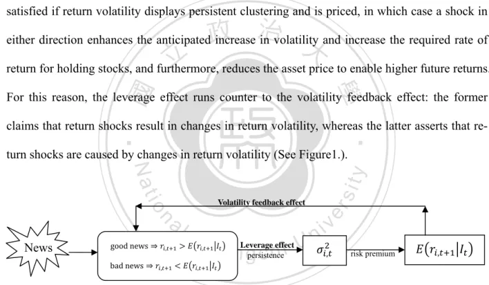
(17) Chapter 2 Time-Changed Lévy Processes with Asymmetric Volatility. tional volatility. Campbell et al. (1997) further put forward asymmetric volatility in light of the leverage and volatility feedback effects. The key research by Black (1976), Christie (1982) claimed that a negative equity return reduces the firm value and thus increases the risk of holding equity, thus increasing volatility risk, under the leverage argument. The volatility feedback effect by Campbell and Hentschel (1992), Bekaert and Wu (2000) and Wu (2001) advocated that it should be satisfied if return volatility displays persistent clustering and is priced, in which case a shock in. 政治大. either direction enhances the anticipated increase in volatility and increase the required rate of. 立. return for holding stocks, and furthermore, reduces the asset price to enable higher future returns.. ‧ 國. 學. For this reason, the leverage effect runs counter to the volatility feedback effect: the former. ‧. claims that return shocks result in changes in return volatility, whereas the latter asserts that return shocks are caused by changes in return volatility (See Figure1.).. n. News. good news bad news. , ,. Ch ,. er. io. al. sit. y. Nat Volatility feedback effect. ni Leverage effect U e n gpersistence , chi. v. risk premium. ,. ,. Figure 1: Unanticipated news impact on asset return volatility.. Although much work has been done for continuous-time stochastic volatility model in Lévy processes (e.g. Carr et al. (2003)), more works need to be conducted to ascertain the leverage effects and volatility feedback effect in asymmetric volatility. Moreover, the requirement of. - 13 -.

(18) Chapter 2 Time-Changed Lévy Processes with Asymmetric Volatility. non-Gaussian specification can be easily grasped by the jump structure of Lévy processes, but stochastic volatility in asset return need to be considered by altering the clock the original process is run. In this paper, I further propose two models as having the asymmetric volatility by introducing unobservable state variable which describes the economic environment and is related to the intensity of trading. 2.3.1 Pure-Continuous Asset Dynamic Process . To model asset price 治政大 time change dynamics, the Brownian motion with drift and the stochastic are in立. is as follows3:. n. al. tion, and continuous integrated stochastic time change. where. Ch. engchi. is a standard Brownian mo-. er. io. 0 represents the initial asset price,. sit. y. Nat. denotes a constant,. 0 exp. ‧. where the process. 學. cluded as:. ‧ 國. Formally, this study denotes the process for the risky asset price by. i Un. v. is given by (1). is considered the state variable of the pure-continuous asset price dynamics, which. is unobservable and is a positive quantity for considering the nature of realistic clock. Carr and Wu (2004) labeled. the instantaneous activity rate.. Following Carr et al. (2003), this study assumes a continuous stochastic time change and spe3. Volatility of Brownian motion with drift is captured by the stochastic time change process tility term could be omitted.. . Hence the vola-. - 14 -.

(19) Chapter 2 Time-Changed Lévy Processes with Asymmetric Volatility. cifies it using the instantaneous activity rate following a CIR mean-reverting square root stochastic process (Cox et al. (1985)):. denotes a standard Brownian motion independent of another Brownian. where tion. . Furthermore, the parameter. controls the speed with which termined by. of the. 立. 治政大 drift Brownian motion with. with the stochastic time. to yield the following expression:. 學. (2). ‧. ‧ 國. change. returns to its long-term mean and the path variability is de-. .. I replace calendar time. is the long-term mean of state variable, while. The driving noise term. of the Eqn. (2) can be transformed into another Brownian. y. sit. n. al. er. io. such that. Nat. motion along the lines proposed by Karatzas and Shreve (1991, p.174) and Mo and Wu (2007),. The following result is obtained:. Ch. engchi. i Un. v. The log-return dynamics is as follows: log Hence the percentage return is given as:. - 15 -.

(20) Chapter 2 Time-Changed Lévy Processes with Asymmetric Volatility. (3) 1⁄2. This study assumes that. where. with constant correlation. and. are two Brownian motions. such that. , thus introducing leverage ef-. fect into the model. The introduction of the CIR dynamic process can help capture the volatility clustering as the required condition for volatility feedback effect, because the instantaneous activity rate. can be considered the instantaneous variance of the Brownian motion.. 政治大. Since the integrated stochastic time change is continuous, the asset return model of Eqn. (3) is. 立. also continuous (Geman et al. (2001)). Additionally, the representation of the asset return be-. ‧ 國. 學. longs to the class of stochastic volatility models, as demonstrated by Ané and Geman (2000).. ‧. 2.3.2 Infinite-jump Asset Dynamic Process. sit. y. Nat. To date, two approaches usually exist in the finance literature for stochastically time-changing. n. al. er. io. original clocks. The first approach has already been documented as preceding context, and the. i Un. v. second is presented below. Additionally, Cont and Tankov (2004) summarize three conventions. Ch. engchi. in relation to building a new Lévy process based on a known one.. Lemma 1: Given a filtered complete probability space Ω , , process on. with characteristic exponent. ists a subordinator subordinated process. and Lévy triplet. with Laplace exponent defined by. ,. , , ,. and Lévy triplet ,. ,. , let. for each. be a Lévy . There also ex-. , 0,. . Then the. Ω is a new Lévy. - 16 -.

(21) Chapter 2 Time-Changed Lévy Processes with Asymmetric Volatility. process with characteristic function given by. and the Lévy triplet. ,. ,. of. is given by. | |. ,. where. 政 .治大. is the probability distribution of. 立. Proof: Please see Sato (1999, p.197) or Cont and Tankov (2004, p.108).. ‧. io. is a Lévy process on. , ,. and let ,. with Lévy triplet. n. al. be a ,. matrix. Then. , where. i n C1h| | 1 :|U engchi | :. be a Lévy. sit. with Lévy triplet. , let. er. Nat. process on. ,. y. ‧ 國. 學. Lemma 2: Given a filtered complete probability space Ω , ,. v. ,. Proof: Please see Sato (1999) or Cont and Tankov (2004, p.105).. To compare two asset return models in terms of portfolio optimization, this study further introduces another way of representing asset prices accompanied by a stochastic process. :. - 17 -.

(22) Chapter 2 Time-Changed Lévy Processes with Asymmetric Volatility. 0 exp where. (4). 0 represents the initial asset price. Economic uncertainty is described by the stochas-. tic process. satisfying (5). and. where. ,. is a constant drift term,. represents a standard Brownian motion. The coefficient ρ allows for correlation be-. 學. ‧ 國. and. 治政 denotes a stochastic time change, 大立. tween the Lévy asset return and changes in volatility.. ‧. To ensure asset return representation exhibits the infinite-jump path behavior, this study ap-. al. and. are independent. The stochas-. er. io. motion with drift. For simplicity, I assume that. sit. y. Nat. plies stochastic time changes resulting from the one-sided pure-jump process to the Brownian. v. n. tic volatility and higher moments are generated by the stochastic time change:. Specifically,. Ch. engchi. i Un. is assumed to be the finite pure-jump Lévy process, which can be ex-. pressed as the difference between two increasing pure-jump Lévy processes: a positive pure-jump Lévy process stochastic time change. and a negative pure-jump Lévy process. . To ensure that a. remains increasing, the negative component is set to zero, that is,. .. - 18 -.

(23) Chapter 2 Time-Changed Lévy Processes with Asymmetric Volatility. Furthermore, the arrival rate of jumps of every positive size time change. in the pure-jump stochastic. is expressed as follows: 1. with the parameter. 0,1 , ,. . The condition. 0,1 is induced by the requirement. is the subordinating process satisfying. that the stochastic time change. 1. ∞. 政治大. Wu (2006) discussed a similar setting including negative jump size . The Lévy density re-. 立 0, and to inverse Gaussian process if. duces to Gamma process if. ‧ 國. ting. 學. coefficient. determines the rate of exponential decay on the right of the Lévy density. By set-. 0 , indicating the absence of exponential dampening, the Lévy density reduces. ‧. to -stable motion as proposed by Mandelbrot (1963). The process. y. Nat. is termed the tem-. io. sit. -stable subordinator which is the Esscher transformed stable subordinator, and. usually termed a normal tempered. n. al. Notably, by setting. is. -stable process (see Cont and Tankov (2004), Chapter 4).. er. pered. 1⁄2. The dampening. Ch. i Un. v. 0, this Lévy density including negative jump reduces to the VG model.. engchi. The parameter simultaneously controls the intensity of jumps of every positive size and transforms the time scale of the dynamic processes. The idea of stochastic intensity of jumps seems to better capture the varying jump structure (Carr et al. (2002)), and is further utilized for optimizing portfolio choice by Cvitanić et al. (2008). Unlike previous studies, rather than indirectly introducing the state variable into the Lévy density resulting from a stochastic time change, as in the VG model, this study employs a more. - 19 -.

(24) Chapter 2 Time-Changed Lévy Processes with Asymmetric Volatility. intuitive approach, which directly introduces the state variable into the stochastic time change describing the change in economic information over time, that is, ,. where. 1. , and. 1. follows CIR dynamic process:. 政治大. The introduction of the CIR mean-reverting square root stochastic process can help capture. 立. stantaneous activity rate. 學. ‧ 國. the volatility clustering as the required condition for volatility feedback effect, because the inalters the intensity of all positive jumps simultaneously. Further-. more, to account for the leverage effect in the asset price dynamics, the second. ‧. nent. in Eqn. (5) is included.. y. Nat. io. sit. Revisiting the Eqn. (5), this study applies Lemma 1 to generate the new Lévy process. n. al. er. which possesses the following Lévy density: ,. Ch. ,. , ,. e| n| g c h i. iv n U ||. 2 (6). where , ,. | |. | | , ,. 2 √2. 2. 2. - 20 -.

(25) Chapter 2 Time-Changed Lévy Processes with Asymmetric Volatility. and. denotes the second kind of modified Bessel function.. Similarly, the Lévy process. has zero diffusion and the drift term is as follows: , | |. The process. | |. can be established by combining two stochastic processes,. which are assumed to be independent for simplicity. Finally, the Lévy triplet. , ,. ,. is given by:. 政治大. ,. √ ,. ,. ,√. ,√. √ ,. ,√. y. Nat. √ ,. io. er. | |. al. n. where. ‧. | |. 學. ‧ 國. 立. sit. for the resulting process. ,. and. Ch. e n g0c h i. i Un. v. and | |. √ ,. ,√. This study gathers all materials to present another representation of asset return such that log. ,. , ,. ,. - 21 -.

(26) Chapter 2 Time-Changed Lévy Processes with Asymmetric Volatility. Percentage return is given by 1. ,. ,. 1 where. ,. ,. denotes the Poisson random measure on Ω. , ,. Lévy density,. When the parameter. related to trading activity or market volatil-. ‧ 國. 政治大 of the Lévy 立 density of the stochastic time change is replaced by the in, the introduction to the CIR dynamic process can help include the. 學. stantaneous activity rate. . Furthermore, its. , captures the varying arrival rate of jumps depending on the informa-. tion of state variable, which represents the current ity.. ,. volatility feedback effect. Additionally, coefficient. considers the presence of the leverage ef-. ‧. fect. In contrast to the pure-continuous model, the infinite-jump asset dynamic process is suita-. Nat. n. sit er. io. al. y. ble to account for periods of high market activity.. Ch. engchi. i Un. v. - 22 -.

(27) Chapter 3 Dynamic Asset Allocation. CHAPTER 3. Dynamic Asset Allocation Next, dynamic asset allocation problem is formally considered, including stochastic asymmetric volatility, using different stochastic time change processes.. 治政 3.1 Investment Opportunity Set and Investor Preference大立 ‧ 國. 學. This section focuses the economic environment in which an investor with CRRA (constant relative risk aversion) utility makes portfolio choices involving two tradable assets: one riskfree as-. ‧. set (money market account) and one risky asset.. Nat. sit. y. Following Merton (1971), I assume that (1) there are no transaction costs and taxes; (2) asset. n. al. er. io. divisibility; (3) the agent is price taker; (4) short sales are allowed; (5) and trading in assets takes. i Un. v. place continuously in time. The stochastic process for the riskfree asset. Ch. engchi. is described by:. where represents the constant instantaneous riskfree interest rate. The stochastic process for the risky asset. has been presented previously, as follows:. Scenario 1: Pure-continuous asset dynamic process (7). - 23 -.

(28) Chapter 3 Dynamic Asset Allocation. Scenario 2: Infinite-jump asset dynamic process 1. ,. ,. (8). Given the stochastic investment opportunity, the agent (fund manager) chooses to invest a fraction. of his funds in the risky asset at each time ,. , and attempts to maximize. the expected utility from terminal wealth with CRRA utility, being given by , if. 0. 政 0, 治if 0大 Regarding the remaining wealth, the proportion 1 , is invested in the riskfree asset. The 立 and maximize. ‧. ‧ 國. Max. sit. Nat. ,. y. his expected utility:. 學. aim of the investor is assumed to care only about wealth at some finite horizon. 0,. 1.. al. n. where. io. on the model choice:. er. subject to intertemporal budget constraints satisfying the self-financing condition, which depend. Ch. e n g c1 h i. i Un. 1,2.. represents investor’s wealth dynamics under the different model ,. 1,2. The investor is endowed with positive initial wealth tion reduces to. v. log. 0 . If. 1, the utility func-. .. - 24 -.

(29) Chapter 3 Dynamic Asset Allocation. 3.2 Pure-Continuous Asset Dynamic Process Likewise, the investor continuously considers how to optimize the allocation of their funds across a risky and riskfree asset. Investor objective function and budget constraint are again given by: Max , subject to the budget constraint. 立. 政1 治大 2. ‧ 國. 學. Following the standard procedure of Merton (1971), Liu et al. (2003) and Liu (2007)4, the value. sit. io. er. ,. y. Max ,. Nat ,. ‧. function (indirect utility function) is defined as. Using the principle of dynamic programming for jump-diffusion processes, the following Ham-. n. al. Ch. ilton-Jacobi-Bellman equation (HJB equation) is obtained,. 0. where. ,. engchi. i Un. v. Max. and. (9). denote the first partial derivatives of. ,. ,. , and so on for higher de-. rivatives. This equation is solved by guessing (then verifying) that the solution to the value function has the following form: 4. More details about technical conditions of HJB equation can be found in Øksendal and Sulem (2005).. - 25 -.

(30) Chapter 3 Dynamic Asset Allocation. ,. ,. (10). Differentiating the above with respect to. , I obtain the following result: in the presence of asymmetric volatility un-. Proposition 1: The optimal portfolio weight. der the pure-continuous stochastic time-changed asset return model in Eqn. (7) is given by , and. 0. for all. (11). satisfy the following system of ordinary differential equations: 1. 1. 0.. 0. (12) (13). ‧. ‧ 國. 1. 1. 學. Proof: See Appendix.. 立. 政治大 1. When the asset return dynamics ignore asymmetric volatility and the stochastic time change is. y. Nat. 0, the investor chooses the following portfolio weight as. io. specified by Merton (1971).. sit. 1 and. n. al. er. omitted, that is,. Ch. engchi. Corollary 1: The optimal portfolio weight. i Un. v. in the absence of asymmetric volatility under. the pure-diffusion stock return model as Merton (1971) is given by5 ,. for all. 0. (14). 5. For comparing to Merton (1971), consumption rate is included in asset allocation problem with power utility. See appendix.. - 26 -.

(31) Chapter 3 Dynamic Asset Allocation. Using the proposition 1, the optimal portfolio choice is determined via two strategies. The first strategy in Eqn. (11) is the mean-variance portfolio or myopic strategy related to the state variable. which describes the current economic information. The second strategy is the. intertemporal asymmetric volatility hedging demand which directly depends on the leverage effect via the correlation coefficient via. . When correlation. , and is indirectly affected by the volatility feedback effect. is nonzero, the investor can hedge expected utility against. asymmetric volatility risk by taking the second holding. Additionally, when the correlation. 政治大. is. zero, namely, ignoring the leverage effect, the intertemporal hedging portfolio strategy imme-. 立. diately disappears regardless of the volatility feedback effect embedded by. . Conversely,. ‧ 國. 學. Chung et al. (2008) claimed the volatility feedback effect is the primary driver of intertemporal. ‧. hedging demand, with the leverage effect playing only a minor role. Notably, the intertemporal. sit. y. Nat. asymmetric volatility hedging demand is independent of the level of the state variable, and in.. io. er. stead is related to the diffusion term of the stochastic time change,. al. A similar hedging strategy for risky assets is surveyed in the finance literature, such as Liu et. n. iv n C h e n gacsimilar al. (2003) and Liu (2007). Wu (2003) proposed h i Uintertemporal hedging strategy based. on the predictability of stock return, which is implicitly embedded in my model setting, as captured by correlation. . On the other hand, the mean-variance portfolio is interpreted as the risky. asset holding against the changes in the financial market. It is inversely proportional to the magnitude of the speed of trading activities, namely,. .. Similar to those of Liu et al. (2003), “market timing” exists for optimizing portfolio choice in relation to asymmetric volatility through the dependence on. . Stated another way, since the. - 27 -.

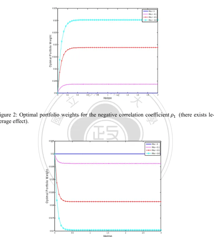
(32) Chapter 3 Dynamic Asset Allocation. state variable alters the original clock using the CIR stochastic process, return volatility is time-varying and clustering. Investment decisions thus are made over a significant horizon. 3.2.1 Numerical Examples This subsection numerically illustrates the implications of asymmetric volatility for optimizing portfolio under the pure-continuous asset dynamic process. The quantitative analyses for the optimal portfolio choice are performed using the following selected parameter values: the state va0.08. 治政大 demand for risky assets for the Figures 2 and 3 illustrate how the leverage effect influences 立. riable. 0.02,. is set to be 0.05,. 2.5 and. ‧ 國. 學. purpose of hedging against the risk caused by changes in investment opportunities. For the numerical example, other parameters should be set besides the parameter equals 5, while. equals 15. This work views the optimal portfolio. ‧. aversion coefficient. . The relative risk. sit. y. Nat. weight as a function of investor horizon measure in years for three different values of the corre-. n. al. timal portfolio weights converge to a constant as. Ch. er. io. lation coefficient, and for both: positive and negative cases. These figures also show that the op-. v. ∞. Notice that intertemporal asymmetric. engchi. i Un. volatility hedging demand disappears when the correlation coefficient. is zero, as mentioned. previously.. - 28 -.

(33) Chapter 3 Dynamic Asset Allocation. 0.5235 Rho = 0 Rho = -0.1 Rho = -0.5 Rho = -0.8. 0.523. O p tim a l P o rtfo lio W e ig h t. 0.5225. 0.522. 0.5215. 0.521. 0.5205. 0.52. 0. 0.2. 0.4. 立. 政治大. 0.6. 0.8. 1. 1.2. 1.4. 1.6. 1.8. 2. Horizon. 0.5205. Nat. Rho = 0 Rho = 0.1 Rho = 0.5 Rho = 0.8. sit. n. al. er. io. O p tim a l P o rtfo lio W e ig h t. y. 0.52. 0.5195. 0.519. (there exists le-. ‧. ‧ 國. 學. Figure 2: Optimal portfolio weights for the negative correlation coefficient verage effect).. 0.5185. Ch. i Un. engchi. v. 0.518. 0.5175. 0.517. 0. 0.5. 1. 1.5. 2. 2.5. 3. Horizon. Figure 3: Optimal portfolio weights for the positive correlation coefficient ative leverage effect).. (there exists neg-. - 29 -.

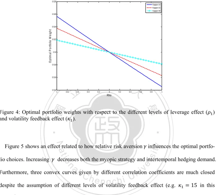
(34) Chapter 3 Dynamic Asset Allocation. Several important features are illustrated. First, the leverage effect is closely related to the optimal portfolio weights for risky assets. When the leverage effect is positive, that is,. 0, de-. mand for risky assets increases with respect to the magnitude of the leverage effect, | |. Fig. 3 shows that demand for assets is inversely proportional to the magnitude of the correlation coefficient, when the leverage effect is negative. 0 .. Figure 4 illustrates the optimal portfolio weight as a function of the level of leverage fect. for different levels of volatility feedback effect. . A larger. 政治大. implies rapid reversion. of the mean to long-term trends, reducing the volatility feedback effect. This result shows that. 立. the dependence of optimal portfolio choice on the volatility feedback effect differs according to. ‧ 國. 學. the condition of the leverage effect. Remarkably, the volatility feedback effect can induce addi-. 0 . Conversely, hedging demand for risky assets occurs when the volatility. y. Nat. 30 but the negative leverage effect dominates the econo-. io. my ρ. sit. feedback effect is not obvious. er. in volatility. ‧. tional hedging demand for risky assets when asset returns are negatively correlated with changes. 0 . When the positive leverage effect exists as documented in the literature, the vola-. al. n. iv n C tility feedback effect implies that rebounds returns are followed by market slumps, h e ningasset chi U. namely, thus volatility involves persistent clustering. The result partially explains why investors prefer to hold low-price assets during the periods of high volatility.. - 30 -.

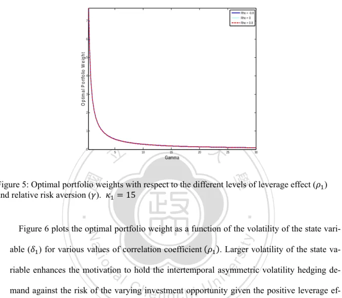
(35) Chapter 3 Dynamic Asset Allocation. 0.528 Kappa=10 Kappa=15 Kappa=30 0.526. O p tim a l P o rtfo lio W e ig h t. 0.524. 0.522. 0.52. 0.518. 0.516. 0.514 -1. -0.8. 立 -0.6. -0.4. 政治大 -0.2. 0. 0.2. 0.4. 0.6. 0.8. 1. Rho. ‧ 國. 學. Figure 4: Optimal portfolio weights with respect to the different levels of leverage effect ( ) and volatility feedback effect ( ).. ‧. Nat. sit. n. al. er. decreases both the myopic strategy and intertemporal hedging demand.. io. lio choices. Increasing. y. Figure 5 shows an effect related to how relative risk aversion influences the optimal portfo-. i Un. v. Furthermore, three convex curves given by different correlation coefficients are much closed. Ch. engchi. despite the assumption of different levels of volatility feedback effect (e.g.. 15 in this. graph)6. Therefore, the leverage effect dominates the volatility feedback effect based on the standpoint of investors considering portfolio optimization.. 6. Other results are available from the authors by request.. - 31 -.

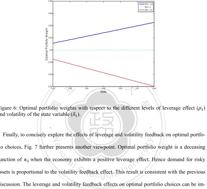
(36) Chapter 3 Dynamic Asset Allocation. Rho = -0.8 Rho = 0 Rho = 0.8. 7. O p tim a l P o rtfo lio W e ig h t. 6. 5. 4. 3. 2. 1. 0. 立 5. 政治大 10. 15. 20. 25. 30. Gamma. ‧ 國. 學. Figure 5: Optimal portfolio weights with respect to the different levels of leverage effect ( ) and relative risk aversion ( ). 15. ‧. io. al. . Larger volatility of the state va-. er. able ( ) for various values of correlation coefficient. sit. y. Nat. Figure 6 plots the optimal portfolio weight as a function of the volatility of the state vari-. riable enhances the motivation to hold the intertemporal asymmetric volatility hedging de-. n. iv n C mand against the risk of the varyinghinvestment i U given the positive leverage efe n g c hopportunity fect. Meanwhile, the motivation for holding intertemporal hedging demand is reduced by the negative leverage effect.. - 32 -.

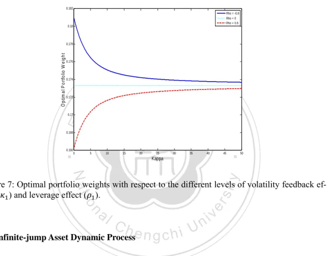
(37) Chapter 3 Dynamic Asset Allocation. 0.524 Rho = -0.8 Rho = 0 Rho = 0.8 0.523. O p tim a l P o rtfo lio W e ig h t. 0.522. 0.521. 0.52. 0.519. 0.518. 0.517 0.02. 立 0.03. 政治大 0.04. 0.05. 0.06. 0.07. 0.08. Delta. ‧ 國. 學. Figure 6: Optimal portfolio weights with respect to the different levels of leverage effect ( ) and volatility of the state variable ( ).. ‧. sit. y. Nat. Finally, to concisely explore the effects of leverage and volatility feedback on optimal portfo-. io. function of. al. er. lio choices, Fig. 7 further presents another viewpoint. Optimal portfolio weight is a deceasing when the economy exhibits a positive leverage effect. Hence demand for risky. n. iv n C assets is proportional to the volatility feedback h e n effect. i Uresult is consistent with the previous g c hThis discussion. The leverage and volatility feedback effects on optimal portfolio choices can be implemented separately in the present example. The case of large. (e.g.. 50) is regarded as. the model without the volatility feedback effect. As reflected in Fig. 7, I observe that the positive leverage effect induces intertemporal hedging demand when the volatility feedback effect is ineffective. From the above numerical examples, the leverage effect mainly induces the intertemporal. - 33 -.

(38) Chapter 3 Dynamic Asset Allocation. hedging demand. The volatility feedback effect works indirectly via the leverage effect and then exerts only a minor influence on asset holding.. 0.182 Rho = -0.8 Rho = 0 Rho = 0.8. 0.18. O p tim a l P o rtfo lio W e ig h t. 0.178. 0.176. 政治大. 0.174. 立. 0.172. 0.168. 0.166. 0. 5. 10. 15. 20. 25. 30. 35. ‧. ‧ 國. 學. 0.17. 40. 45. Kappa. Nat. y. 50. sit. n. al. er. io. Figure 7: Optimal portfolio weights with respect to the different levels of volatility feedback effect ( ) and leverage effect ( ).. Ch. engchi. 3.3 Infinite-jump Asset Dynamic Process. i Un. v. Similarly, the investor also faces the same objective function, with different budget constraint. Investor objective function and budget constraint are given by: Max , subject to the wealth dynamics,. - 34 -.

(39) Chapter 3 Dynamic Asset Allocation. 1. ,. ,. Following the standard procedure of Merton (1971), this study also defines the value function as ,. Max ,. ,. As usual, applying the principle of dynamic programming for Lévy processes, one can yield the following HJB equation,. 0. 政治大 1 , ,. Max. 立1 and. ,. denote the first partial derivatives of. ‧ 國. ,. , ,. 學. where. (15) ,. ,. , and similarly for higher. derivatives. Following Cvitanić et al. (2008, eq. 46), the equation is solved by guessing (and. ‧. verifying) the solution to the value function has the following separable functional form:. y. ,. io. , I reach the following result:. n. er. Differentiating the above with respect to. al. Ch. Proposition 2: Assume that a solution weight. (16). sit. Nat. ,. engchi. i Un. v. to Eqn. (15) exists. Then the optimal portfolio. in the presence of asymmetric volatility under the infinite-jump stochastic. time-changed asset return model in Eqn. (8) is given by 1. 1. 1. 0,for all. 0. (17). Also. - 35 -.

(40) Chapter 3 Dynamic Asset Allocation. | |. √ ,. ,√. where. and , ,. | |. 2. 1. , and. Proof: See Appendix.. 立. 政治大. Proposition 2 indicates that the optimal portfolio weight. ‧ 國. 學. state variable. for risky assets depends on the. because of the implicit relationship shown in Eqn. (17). In contrast to the. ‧. findings of Benth et al. (2001), namely that optimal portfolio choice is a fixed fraction of wealth. sit. y. Nat. over time, the finding of Benth et al. can be considered my special case in the situation where. io. al. er. the stochastic time change (implicitly including volatility feedback effect) and leverage effect are eliminated. In contrast to Cvitanić et al. (2008), present study builds on previous research. n. iv n C U h e nbygdirectly ensuring agreement with more stylized facts the calendar time into the c h i transforming business time, and allowing for the dependence between the time-changed Lévy process and the state variable. In conclusion, the optimal portfolio weight. is a deterministic function of. . There-. fore, once the expectation of the state variable is known, the long-term policy of asset allocation, namely, the expectation regarding the optimal portfolio choice, is determined.. - 36 -.

(41) Chapter 3 Dynamic Asset Allocation. For simplicity this study applies the conditional cumulant exponent. , as previously applied. by Cvitanić et al. (2008) and Wu (2006), which is defined as 1. ,. The unconditional version is 1 Then. 政治大. 立. is obtained by 1. ,. 2. ‧. 2. 學. ‧ 國. The instantaneous variance of percentage returns. 1. n. al. er. io. sit. y. Nat. Next, I present the following proposition:. Ch. Proposition 3: Assume that the ratio ⁄. Eqn. (8), that is,. ⁄. engchi. i Un. v. is a constant under the Model 2 in. . Then the optimal portfolio weight. is indepen-. dent of state variable, and satisfies 2. 2. 1. 1. 1. 1. 0, for all. 0 (18). where. and. - 37 -.

(42) Chapter 3 Dynamic Asset Allocation. , ,. | |. 2. 1 Proof: Refer to Cvitanić et al. (2008).. is determined without the state variable information, which de-. From the Eqn. (18),. scribes the randomness of the economic environment. The independence of the optimal portfolio weight from. 政治大. stems from the fact that stochastic risk premium,. 立. to the instantaneous rate of variance. , is proportional. and the randomness of the Lévy density under the. ‧ 國. 學. present study. Similar results are presented in the finance literature, such as Liu et al. (2003) and. ‧. Cvitanić et al. (2008). More importantly, the results claim that the channel for influencing the. sit. y. Nat. asymmetric volatility based on volatility feedback effect is ignored. The leverage effect becomes. io. er. the only cause for the intertemporal asymmetric volatility hedging demand, thus implying that the leverage effect plays a major role for portfolio optimization in this situation.. n. al. ble. engchi. ⁄. Remark: Assuming that interest rate. Ch. i Un. v. is constant means that the constant riskfree. is relaxed to be the stochastic process proportional to the positive state. , that is,. 2. 2. 1. .. - 38 -.

(43) Chapter 3 Dynamic Asset Allocation. 3.3.1 Reduced Time-Changed Lévy Process To illustrate asymmetric volatility risk effect upon optimal portfolio choices using time-changed Lévy processes, particularly for leverage and volatility feedback effects, this study works with a reduced form of general time-changed Lévy process and numerically explores adjustment mechanism related to optimizing portfolio given varied asset return volatility. As mentioned previously, VG and NIG models can be considered time-changed Lévy processes by altering the calendar time used to run a Brownian motion with drift. In contrast to. 政治大. these models, CGMY of Carr et al. (2002) was adapted by directly specifying the Lévy density,. 立. 學. ‧ 國. and it is unclear whether this process can be built as a time-changed Brownian motion. Madan and Yor (2008) presented the findings to answer this question.. ,. , and. :. y. Nat. io. 1. al. | |. n. where. 0,. 0,. the stochastic time change. sit. ,. 0, and. Ch. 1. | |. engchi. er. with parameters. ‧. To extend VG model to more general cases, Carr et al. provided the following Lévy density. i Un. v. 2. Based on the derivation of Madan and Yor (2008),. related to CGMY is absolutely continuous with respect to. one-sided stable ⁄2 subordinator with the following Lévy density: 1 ⁄ ⁄. - 39 -.

(44) Chapter 3 Dynamic Asset Allocation. 2 2 1 2 where. ⁄. ,. ⁄. 4. 1. are two independent gamma variates with unit scale parameters and shape pa-. rameter ⁄2, 1⁄2 respectively. Next, the above expectation term can be explicitly evaluated, as follows:. ,. 2. ,. 2. ‧. ‧ 國. 2. ⁄. n. al. Ch. sit. .. 2. er. io. is the Hermite function with parameter. y. 2. Nat. , , and. ⁄ ⁄. 學. where. 立. 政治大. i Un. v. Applying the results of Madan and Yor (2008), this study defines a state-dependent Lévy den-. engchi. sity for the stochastic time change to reduce the general case, as follows: ·. ,. ·. ⁄ ⁄. ·. 1. where. - 40 -.

(45) Chapter 3 Dynamic Asset Allocation. ⁄ ⁄. ·. ·. 1. and. . The. can then be replaced by reduced GMY (state-dependent) Lévy. density such as: 1 | |. | |. 1. 治政 . The parameters and 大 control the sign of skewness of dis立. and. , the rate of exponential decay on the right of the Lévy density is. 學. ‧ 國. tribution function. For. larger than the left, leading to the fact that large negative realizations are more likely to appear. ‧. than large positive realizations, namely, negative skewness. Following numerical examples. y. sit. io. al. er. uation.. Nat. concerning unsymmetrical time-changed Lévy process are provided within the scope of this sit-. v. n. Inspecting the above equations, the model of Cvitanić et al. (2008) is naturally adopted as my. Ch. i Un. e n g c h 0.i Assuming that. special case if the leverage effect is ignored and. | |. ∞, this study is simplified as much as possible in the numerical examples. From the results of Wu (2006) and Madan and Yor (2008)7, this work immediately determines that log 2. cos. (19). 7. Wu (2006) ignored the truncation function in the characteristic function and regarded CGMY model as their special case.. - 41 -.

(46) Chapter 3 Dynamic Asset Allocation. 2 tan The reduced CGMY model is infinite-jump time-changed Lévy process. I then obtain the following results.. 政治大 rived by Madan and Yor (2008), the optimal portfolio weight 立. Corollary 2: When the time-changed Brownian motion with drift follows the CGMY model de-. 1. 1. 1. ,. 1. for all. 0.. (20). Nat. er. io. sit. y. 1. ‧. 0. ‧ 國. Then. 1. 學. 1. in Eqn. (17) reduces to. This investigation focuses on the implicit relationship in Eqn. (20) between the long-term. al. n. iv n C policies of asset allocation and the volatility effect . Chacko and Viceira (2005) and h e nfeedback gchi U. Wachter (2002) stressed the importance of mean-reverting asset returns for portfolio optimization. Therefore, the reduced form of the general model is conducted by the desire to develop a simple framework in which the optimal portfolio problem can be explored in the presence of asymmetric volatility, especially for the leverage and volatility feedback effects. 3.3.2 Numerical Examples This subsection illustrates the implications of asymmetric volatility for optimizing portfolio un-. - 42 -.

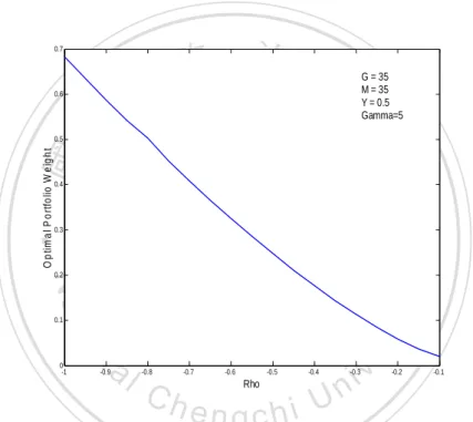
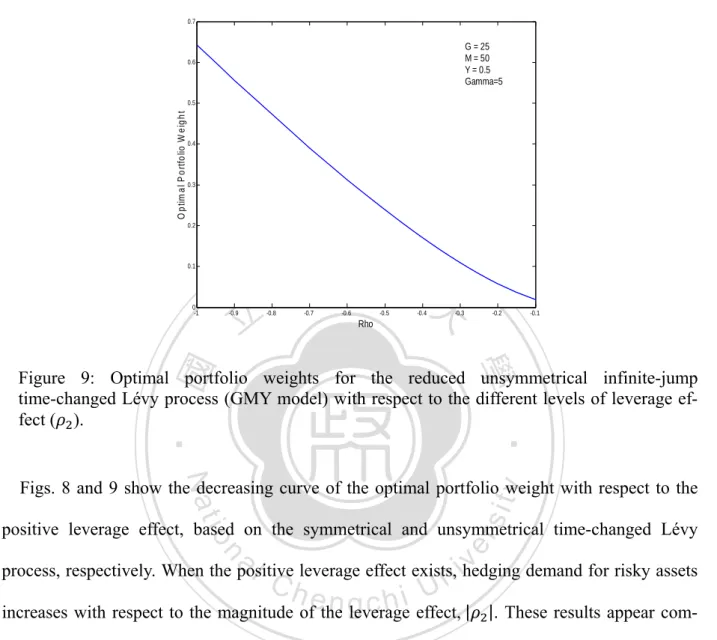
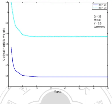
(47) Chapter 3 Dynamic Asset Allocation. der the Proposition 3 and the reduced form of the infinite-jump dynamic process. First of all, Figure 8 shows the symmetrical state-dependent CGMY (GMY model) using the Proposition 3, that is,. , in which the correlation coefficient. cal studies, with the mean-reverting state variable. is negative as documented in the empiri, to enable simultaneous leverage effect and. volatility feedback effect.. 政治大. 0.7. 立. 0.6. G = 35 M = 35 Y = 0.5 Gamma=5. 0.5. ‧. O p tim a l P o rtfo lio W e ig h t. ‧ 國. 學. 0.4. 0.3. sit. y. Nat. 0.2. io. al. n. 0 -1. -0.9. er. 0.1. -0.8. -0.7. Ch. -0.6. -0.5. Rho. -0.4. engchi U. v ni -0.3. -0.2. -0.1. Figure 8: Optimal portfolio weights for the reduced symmetrical infinite-jump time-changed Lévy process (GMY model) with respect to the different levels of leverage effect ( ).. - 43 -.

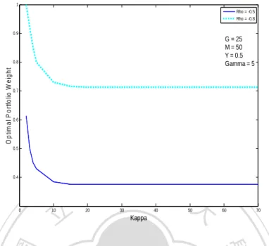
(48) Chapter 3 Dynamic Asset Allocation. 0.7. G = 25 M = 50 Y = 0.5 Gamma=5. 0.6. O p tim a l P o rtfo lio W e ig h t. 0.5. 0.4. 0.3. 0.2. 0.1. 0 -1. 立. -0.9. -0.8. 政治大 -0.7. -0.6. -0.5. -0.4. -0.3. -0.2. -0.1. Rho. ‧ 國. 學. ‧. Figure 9: Optimal portfolio weights for the reduced unsymmetrical infinite-jump time-changed Lévy process (GMY model) with respect to the different levels of leverage effect ( ).. Nat. sit. y. Figs. 8 and 9 show the decreasing curve of the optimal portfolio weight with respect to the. n. al. er. io. positive leverage effect, based on the symmetrical and unsymmetrical time-changed Lévy. i Un. v. process, respectively. When the positive leverage effect exists, hedging demand for risky assets. Ch. engchi. increases with respect to the magnitude of the leverage effect, | |. These results appear compatible with the pure-continuous variation case, despite signs of skewness in distributions of asset returns. To examine the long-term influence of the volatility feedback effect on policies of asset allocation, some numerical examples inevitably need to be executed based on the reduced model8.. 8. This study assumes the interest rate equals 0.01.. - 44 -.

(49) Chapter 3 Dynamic Asset Allocation. 1.1 Rho = -0.5 Rho = -0.8 1. G = 35 M = 35 Y = 0.5 Gamma=5. O p tim a l P o rtfo lio W e ig h t. 0.9. 0.8. 0.7. 0.6. 0.5. 0.4. 立. 0. 10. 20. 政治大 30. 40. 50. 60. 70. Kappa. ‧ 國. 學. Figure 10: Optimal portfolio weights for the reduced symmetrical infinite-jump time-changed Lévy process (GMY model) with respect to the different levels of volatility feedback effect ( ).. ‧ sit. y. n. al. does induce the intertemporal hedging. er. under the symmetrical GMY model. Decreasing. io. of. Nat. Figure 10 shows that optimal portfolio weight is inversely proportional to the value. i Un. v. demand. Consequently, the volatility feedback effect motivates hedging demand for risky assets. Ch. engchi. due to the asset volatility clustering embedded in the stochastic time change. These results greatly resemble those demonstrated in the pure-continuous variation case. Figure 11 also provides the similar results.. - 45 -.

(50) Chapter 3 Dynamic Asset Allocation. 1 Rho = -0.5 Rho = -0.8 0.9. G = 25 M = 50 Y = 0.5 Gamma = 5. O p tim a l P o rtfo lio W e ig h t. 0.8. 0.7. 0.6. 0.5. 0.4. 立. 0. 10. 20. 政治大 30. 40. 50. 60. 70. Kappa. ‧ 國. 學. Figure 11: Optimal portfolio weights for the reduced unsymmetrical infinite-jump time-changed Lévy process (GMY model) with respect to the different levels of volatility feedback effect ( ).. ‧ y. sit. n. al. er. to be 0.25, namely, a short-term investment horizon. When the investment decision. io. meter. Nat. Several points are worth noting. The experiments presented in Figs. 10 and 11 set the para-. i Un. v. horizon is lengthened, the influence of volatility feedback effect on optimal portfolio choice is. Ch. engchi. reduced9. This may be due to the fact the volatility feedback effect will be offset over the long-term investment horizon. Finally, similar to the results in Fig. 3, increasing. reduces the. optimal portfolio weight. In a word, my findings are crucial in clarifying how the leverage and volatility feedback effects influence optimal portfolio choices for investors beyond stochastic volatility in financial theory. This study mainly highlights the importance of the well-known stylized fact, asymmetric 9. The results are available from the authors by request.. - 46 -.

(51) Chapter 3 Dynamic Asset Allocation. volatility, for determining the risky asset holdings in dynamic asset allocation. According to the numerical examples and discussions, the (positive) leverage effect also induces the intertemporal hedging demand. The volatility feedback effect just works over the short-term investment horizon. Restated, the leverage effect plays a major role for portfolio optimization.. 立. 政治大. ‧. ‧ 國. 學. n. er. io. sit. y. Nat. al. Ch. engchi. i Un. v. - 47 -.

(52) Chapter 4 Empirical Results. CHAPTER 4. Empirical Results Several studies (e.g. Carr et al. (2002) and Geman (2002)) examined whether the diffusion term needs to be included when modeling asset returns given the ability of infinite-activity jump. 治政大 large moves. This section asstructure to describe both frequent small moves and occasional 立. sesses the asymmetric volatility to explore the proposed general asset return model, which em-. ‧ 國. 學. ploys stochastic time changes associated with both jump and diffusion components by calibrat-. ‧. ing model parameters to U.S. equity index returns. Unlike previous studies, this investigation. sit. y. Nat. particularly answers this problem by adding two different drivers to asymmetric volatility,. io. al. er. namely, diffusion and jump components. The section is structured as follows: first, this section. iv n C U section describes the data source h e n gSecond, time changes via two distinct driving channels. c h i this n. presents the general stochastic asymmetric volatility asset return model by utilizing stochastic. and illustrates the use of spectral GMM estimation by Chacko and Viceira (2003) to calibrate the parameters of the proposed general stochastic asymmetric volatility asset return model. 4.1 The General Stochastic Asymmetric Volatility Model To deal with this issue, this study denotes the asset spot price at time as. . Following the. preceding discussion, the general stochastic asymmetric volatility model is proposed as follows:. - 48 -.

(53) Chapter 4 Empirical Results. 0 exp. (21). : State-dependent subordinating Lévy process, where. ,. denote the distinct stochastic time changes as mentioned before, which are. mutually independent,. represents a Brownian motion with drift and. Brownian motion independent of. 立. is a standard. . Carr et 治 al. (2002) presented an exploration regarding 政大. the employment of diffusion in their framework. In contrast to Carr et al., this work considers. ‧ 國. 學. the well-cited stylized fact, asymmetric volatility, via stochastic time changes. This study aims to improve the understanding of the use of diffusion term for financial modeling under the. ‧. and. . The state variable. n. al. , the variation of asset price is controlled by two. sit. io. state variables, represented by. and. er. Nat. In the above model, besides. y. framework of the time-changed Lévy process10.. nuous shock. Ch. i Un. v. underlying the conti-. captures the leverage effect by allowing for negative correlation. The pro-. engchi. posed model then considers the volatility feedback effect by setting. as a CIR. mean-reverting square root stochastic process. Meanwhile, the state variable. underlying. the jump structure captures both the leverage and volatility feedback effects as described above. Particularly, two state variables are unobservable in the market. By applying two stochastic time 10. This work omits the term ‘convexity correction’ due to access the relevance of the diffusion term from the evolu-. tion of statistical process.. - 49 -.

(54) Chapter 4 Empirical Results. changes to the Brownian motions (with drift), the proposed asset return model emphasizes that stochastic asymmetric volatility is driven by multiple sources of random shock. According to the general model specifications, the extended model of Carr et al. (2002) with a diffusion is adopted as a special case when the stochastic time change while. is constant,. remains random as proposed by Madan and Yor (2008), and asymmetric volatili-. ty(e.g. leverage effect and volatility feedback effect) is ignored. On the other hand, VG model is evolves like Gamma. also my special case similar to those of Carr et al. (2002), but process.. 立. 政治大. Formally, this work permits the separate treatment of the pure-continuous and infinite-jump. ‧ 國. 學. time-changed Lévy processes to enable the generation of stochastic asymmetric volatility via. ‧. both components.. sit. y. Nat. 4.2 Data and Model Parameter Estimation. n. al. er. io. This study uses the S&P 500 index data from January 1, 1980 to June 30, 2008 at two different. i Un. v. frequencies, daily and weekly, to estimate the proposed general stochastic asymmetric volatility. Ch. engchi. asset return model, based on the characteristic function with spectral GMM estimation proposed by Chacko and Viceira (2003).. - 50 -.

(55) Chapter 4 Empirical Results. 0.05. log-return. 0. -0.05. -0.1. -0.15. -0.2. 立 1000. 2000. 3000. 4000. 5000. 6000. 7000. 學. days. ‧ 國. -0.25. 政治大. ‧. Figure12: Daily S&P index log-return, from January 1, 1980 to June 30, 2008.. y. Nat. er. io. sit. Numerous studies have estimated the parameters of the stochastic volatility model through the characteristic function methods, such as Singleton (2001), Jiang and Knight (2002) and Chacko. n. al. Ch. i Un. v. and Viceira (2003). Among these studies, spectral GMM estimation is particularly suitable for. engchi. time-changed Lévy processes because of its direct use of characteristic function without inversion to recover the density function and closed form of the return moment. Generally, few estimation methods using the traditional maximum likelihood are easy to be use because no analytical expression is known for the density function of the time-changed Lévy process, as the model presented here. Therefore, to respond to the above difficulty, this study employs spectral GMM to estimate the parameters of the general stochastic asymmetric volatility asset return. - 51 -.

(56) Chapter 4 Empirical Results. model. First, the conditional characteristic function. , ; , log. must be defined as follows:. , ; , log cos where. log. , log. , log. sin. log. , log. (22). 0. The Eqn. (22) de-. is a vector of parameters of the general asset return model,. notes the Euler expansion of exponential of complex variable. The definition of the conditional. 政治大. characteristic function implies. 立. 0. (23). ‧ 國. 學. for all. , ; , log. . The Eqn. (23) defines an infinite set of complex-valued moment conditions. The. following pair of real-valued moment conditions can be induced: , ; , log. log. , ; , log. 0. io. n. al. 0. (24). er. Im exp. sit. y. log. Nat. ‧. Re exp. v. where Re · and Im · are real-valued operators that extract the real and imaginary parts of the complex to. , ;. number.. The. Ch. r-dimensional. instrument. log. ,. orthogonal. is given as follows: log. where. evector n g c hofi. i Un. , ;. exp. log. ,. , ; , ; , log. 0 . Furthermore, the above ex-. pression can be considered the complex-valued moment conditions implying the following pair of real-valued moment conditions:. - 52 -.

(57) Chapter 4 Empirical Results. Re. log. ,. , ;. 0. Im. log. ,. , ;. 0. ,. Choosing a set of appropriate points for. ,…,. , the pair of real-valued moment. conditions can be obtained as ; log ; log. where. ,. denotes a 2. log. ;. 立. ,. ,. ;. ,…,. ,. ;. , ;. is an n-dimensional vector orthogonal. 學. to. ,. , ;. ‧ 國. , ;. 1 vector of moment condition satisfying Re log , 治政 Im log , 大. ; and. 0. , .. ‧. Based on the above discussion, Chacko and Viceira (2003) treat above transformation as the. sit. y. Nat. standard procedure involved in the GMM estimation. Given a set of index data observed at a. n. al. ; log. C, h. er. io. discrete time, the corresponding sample moment conditions is denoted as 1. engchi. Spectral GMM estimation identifies values of. i Un. ; log. v. that make the sample moment condition as. close to zero as possible, based on the following quadratic form: arg min. SGMM. where. ; log. ,. ; log. ,. ; log. ,. ; log. ,. denotes a positive-definite, symmetric weighting matrix. Similar to the. properties of GMM, the asymptotic variance of the spectral GMM estimator is minimized when. - 53 -.

(58) Chapter 4 Empirical Results. choosing the following weighting matrix: ; log ; log. where. ,. ; log. timator to replace the. ; log ,. , ,. . In fact, I can find any consistent es-. .. The conditional characteristic function is defined as follows: , ; , log. ,. , log. ,. 1,2.. Next, this study integrates the unobservable state variable in the asset return model out of the. 政治大 above conditional characteristic function to yield the characteristic function based only on cur立. ‧ 國. 學. rent asset price. The conditional characteristic function should be provided to estimate the parameters of the proposed general asset return model via the Kolmogorov backward equation11.. ‧. The conditional characteristic functions of the pure-continuous and infinite-jump stochastic. sit. y. Nat. time-changed asset price models are prioritized in calibrating the general stochastic asymmetric. n. al. er. io. volatility asset return model.. Ch. engchi. i Un. v. Proposition 4: If the asset percentage return is introduced as Eqn. (7), then the conditional cha, ;. racteristic function log. , ;. , log. , log log. satisfies the following analytic expression: , ;. log. , ;. (25). where 11. Further details of the Kolmogorov (forward-) backward equation and their applications are presented in Ma and. Yong (1999).. - 54 -.

(59) Chapter 4 Empirical Results. ,. ,. ,. ,. , ; , ;. log 2 2. Proof: See Appendix.. 立. 政治大. , ;. , ;. , log. , log. ,. ,. satisfies the following analytic expression:. ‧. log. ‧ 國. racteristic function. 學. Proposition 5: If the asset percentage return is introduced as Eqn. (8), then the conditional cha-. log. y. Nat. sit. n. al. er. io. Furthermore,. Ch , log. , ;. log. 2. e nlog gchi. i Un. v. log. , ;. (26). where , , , ;. ,. ,. ,. , 2. Proof: Refer to Cont and Tankov (2004, p. 115) and the Appendix of the Proposition 4.. - 55 -.

(60) Chapter 4 Empirical Results. The results of Propositions 4 and 5 easily lead to the following expression regarding the conditional characteristic function of the general time-changed asset price dynamics with asymmetric volatility.. Proposition 6: If the asset price dynamics is given as Eqn. (21), then the conditional characte-. ,. ,. ,. Nat. , ;. log. ,. ,. ,. al. n. , ;. io. , ;. ,. , ;. (27). y. ,. log. , ;. ‧. , ,. 立. , ;. 學. where. , log. 治政 log log 大. ‧ 國. , ;. satisfies the following analytic expression:. sit. log. , ; , log. er. ristic function. Ch. engchi. i Un. v. 2. With the closed-form conditional characteristic functions as described above, spectral GMM estimation can be applied in the proposed general stochastic asymmetric volatility asset return. - 56 -.

(61) Chapter 4 Empirical Results. model.. Table 1: The spectral GMM Estimates of the General Continuous-time Time-changed Asymmetric volatility Model. Daily Data. Model parame-. Weekly Data. Estimates. SE. p-value. 0.811855**. 0.036300. 0.000000. 82.615909**. 30.721756. 0.767493**. 0.367373. -0.348467**. 0.004590. Estimates 0.942102**. 66.147332** 0.007179 治政大 0.754793 0.036729. SE. p-value. 0.014586. 0.000000. 15.646848. 0.000025. 0.461611. 0.102236. 0.000000. -0.434598**. 0.133070. 0.001116. 學. 立. ‧ 國. 0.025543. 0.772264*. 0.412224. 0.061210. 63.253463**. 0.538977. 0.000000. 48.152096**. 20.409658. 0.018440. 74.069214**. 10.143394. 0.000000. 101.865132**. 27.397853. 0.000208. 0.539658**. 0.058467. 0.000000. 0.880970**. 0.152962. 0.000000. 0.075333. 0.000000. 0.421849**. 0.082872. 0.000000. 0.000204. 0.057222*. 0.033777. 0.090460. 0.025903. 0.004381. io. 0.013523**. 0.003640. n. al. y. sit. 0.446344**. ‧. 0.371334. Nat. 0.829387**. er. ters. i n C U hengchi *denote an estimate that is significant at 95% level. 0.078087**. 0.022087. 0.000410. v. 0.073922**. ** denote an estimate that is significant at 90% level.. Table 1 lists the model parameter estimates, together with their standard errors (SE) and p-values. This table clearly indicates that stochastic asymmetric volatility and infinite-jump structure need to be included to describe the asset price dynamics. The coefficients for the pure-continuous and infinite-jump time-changed components are statistically significant in daily. - 57 -.