行政院國家科學委員會專題研究計畫 成果報告
不動產估價師部分調整行為之研究
研究成果報告(精簡版)
計 畫 類 別 : 個別型 計 畫 編 號 : NSC 98-2410-H-004-132- 執 行 期 間 : 98 年 08 月 01 日至 99 年 07 月 31 日 執 行 單 位 : 國立政治大學地政學系 計 畫 主 持 人 : 陳奉瑤 計畫參與人員: 碩士班研究生-兼任助理人員:廖彬傑 碩士班研究生-兼任助理人員:徐笠嫻 報 告 附 件 : 出席國際會議研究心得報告及發表論文 處 理 方 式 : 本計畫可公開查詢中 華 民 國 99 年 10 月 11 日
1
1. 前言
此次金融海嘯席捲世界造成重大傷害,突顯出經濟景氣循環中繁榮階段的過 度樂觀與泡沫化,其似乎隱現投資人具動物本性(animal spirit),有追高助跌的行 為,也引發對估價平滑評判的再省思。不動產估價師應於市場中扮演提供合理價 值資訊的角色,如果如同 Fisher et al.(1999)與 Geltner(1998)之主張,估價 師於景氣繁榮階段的估值傾向低於真實成交價格;景氣衰退時,估值相對高於成 交價格,那麼呈現的估價平滑是一種偏誤,抑或是理性預期(rational expectation) 的行為?如果以估值基礎指數小於成交資料指數變異程度或呈落後現象予以論 斷,屬於前者的思維;但若就景氣循環觀察並深究估價師部分調整的成因,或有 不同的發現。尤其,華人受財產偏好觀念的影響,對於不動產增值利得的重視遠 甚於持有期間的租金收益,房價追高助跌的情形時有所聞,此時估價師的部分調 整行為是否理性,是否因市場的不確定性增加而更趨保守,值得深入探究。 本文除前言外,首先回顧估價平滑與部分調整之相關文獻,進而運用 T-REITs 之信託資產重新估價案例為對象,調整 Quan and Quigley(1991)提出之部分調 整模型,除藉以驗證估價師是否採取部分調整的重新估價策略外,並進而做為推 論該部分調整行為是否因市場不確定性的增加而更趨保守的基礎,經實證分析 後,最後提出結論。2. 文獻回顧
價格部分調整,意指有估價平滑現象。早期有關估價平滑之相關研究,由於 研究者僅能獲得估值資料,當估值報酬偏離或未能及時反映市場價值或報酬變動 時,偏誤的資料將會造成風險性的判斷錯誤,導致錯誤的投資決策,對於基金投 資人影響甚鉅。故文獻上多以估值指數相對落後於成交價格指數觀察(Geltner, 1989a ;Fisher et al., 1999),並研究不同方法設法改進平滑因子(Ross and Zisler,1987;Geltner, 1989b),發展去平滑技術,以得到相對較「真實」的不動產價格
指數或報酬序列,進而和其他投資組合進行風險的比較分析,而此等文獻多從總 體角度進行分析。
2 Matysiak, 1998),且不同不動產類型與估價報告書使用方式,所造成的效果皆不 同,並不能就過去推論某資料具有估價平滑現象便一概而論,且以偏誤的觀點移 除平滑效果時,隱含造成估價平滑原因來自估價師誤用方法或能力不足,係導因 於估價師「未能」確實掌握市場變動而造成估值偏離市場成交價格。誠如 Brown and Matysiak(1998)所言,參考太多過去資訊的估價結果,將出現強烈自我迴 歸而產生估價平滑。
Lai and Wang(1998)提出相反的見解,認為先前的探討多受限於估價平滑 確實存在變異程度較小的錯誤假設,以致運用去平滑後的總體資料估計估值報酬 反隱含更高風險。雖然 Geltner(1998)認為 Lai and Wang(1998)混淆了個體層 級誤差的概念,導致錯誤的推論,但也肯定在未完全瞭解估價平滑,就主張去除 估價平滑是相當危險的,並建議未來朝向估價行為等其他觀點探討。
Quan and Quigley(1991)強調估價師應能從紛亂的市場訊息中獲得有用的 資訊,其以為估價師採取保守的部分調整策略符合理性行為,而減少價格變異程 度也是估價師存在的價值之一。Clayton et al.(2001)則異於過去運用總體資料 之文獻,改由個別估價報告書萃取相關資料,應用 Quan and Quigley 的部分調整 模型(rational partial adjustment model),將信心程度設定為估價師可得市場資料 的函數,結果發現估價師的信心程度因時而異,在不同的景氣循環階段下估價師 進行更新調整幅度不一,其主張去平滑不應以固定參數方式進行,並建議資產經 理人定期更換估價師以減少估值的延遲效果。 除實證分析外,Mcallister et al.(2003)深度訪談英國估價師發現,估價師 和其所處的外在環境形成一個複雜的回饋系統,估價師與客戶互動將會影響資產 的績效,尤其在資產價值下跌期間,由於缺乏市場改變的證據,估值傾向維持不 變。顯然週期性估價比其他估價更容易受到客戶影響。基此,本文期望跳脫總體 指數資料的分析方式,藉由重新估價的資料深入分析估值與估價師部分調整行為 的關係。 過去提及估價平滑的構成原因,可能因為估價師依賴先前成交價格(Ibbotson and Siegel, 1984)或前期估值(Ross and Zisler, 1987; Geltner, 1989),估價師在心 理上受到過去估價結果的限制,導致估值指數具有延遲的自我迴歸。Geltner (1998)則依據隨機誤差和不動產報酬的關係將隨機誤差分為兩類,一為和不動
3 產報酬無關的隨機誤差,另一為和不動產報酬呈負相關之隨機誤差。前者因估價 師之差異或所處之外在環境所造成;後者則表示當市場景氣佳時,不動產報酬為 正,估值傾向低於真實成交價格,發生低估之隨機誤差,當報酬為負則發生高估 誤差。其認為後者為造成估價平滑的主因,而造成該種誤差之可能原因即為估價 師依賴過去資訊之行為。然而此等研究並未明確指出造成估價平滑的原因,僅能 提出一個模糊的可能見解,無法具體分析先前價格或估值如何影響估價師的調整 行為。
Quan and Quigley(1991:138)認為市場成交價格受到買賣雙方資訊不同、 議價能力差異等影響,因而估價師之角色未必完全反應市場成交價格,因而提出 部分調整模型。其認為市場噪音越大,則市場上觀察到的成交案例狀況越分歧, 估價師越難發現市場變動趨勢,不易在估價程序中獲取適當的比較案例,或必須 進行較多的調整修正而提高估價的不確定性;因此,估價師信心越低,給予市場 資訊的權重越小,表示越依賴前期估值。 有關信心程度之大小,Diaz(1997)對市場資訊信心程度雖然高達0.88,但 其中有相當比例係來自估價人員對地理環境的熟悉度;此與Diaz and Hansz (1997)之研究相較之下可發現,地理環境熟悉度約佔0.3;而Diaz and Wolverton (1998)對資深估價人員進行的實驗中發現,重新估價人員較第一次估價者對市 場的依賴程度相對較小,依Hansz 計算之信心程度為0.70;Hansz(2004)給予 估價人員不同之前次移轉價格,發現估價人員對高價群組之前次移轉價格信心較 低0.48,對低價群組較高0.66。前述研究皆以控制實驗方式進行,Clayton et al. (2001)則以加拿大33個不動產共202個重新估價報告書進行實證分析,其認為 估價師對市場資訊的信心程度並非固定參數,將因大環境干擾、是否更換估價師 等外在影響而異,若以所有資料之平均數試算,參考前期估值之信心程度約 0.69;參考其他估價人員估值之信心程度為0.87。基本上因研究方法、參考點以 及對市場的熟悉程度而有不同的效果。本文將以T-REITs之投資資產為分析客體 進行實證分析,基本上執行估價之估價師對此市場皆有相當的熟悉度,且依規定 三年才需更換估價機構而缺乏足夠資料進行分析,因此,將不就市場熟悉度和是 否更換估價師分析其信心效果。然而Levy and Schuck(1999)認為估價非僅不動 產特徵價值化的結果,事實上尚包含非價格資訊的影響。而過去相關研究,主要 則由定錨與客戶影響之估價行為討論估價平滑。
4
定錨(anchoring )指行為人傾向找一個量化參考值作為評估基礎,判斷時 不自覺地使用該數值為基準進行調整,由於受到參考點的影響,通常會發生調整 不足的現象(Kahneman and Tversky, 1973)。文獻中探討之參考點包括:前次成 交價格(Hansz, 2004)、其他估價師估值(Diaz, 1997;Diaz and Hansz, 1997; Clayton et al., 2001)以及前期估值(Cole, 1986;Diaz and Wolverton, 1998;Clayton et al., 2001)。除前述參考點之定錨外, Levy and Schuck(1999)認為老練客戶 可能透過資訊的力量影響估價結果;而較不老練的客戶,則傾向運用獎賞、高壓 或煩擾的方式對估價人員施壓;Chen and Yu(2009)以台灣與新加坡估價師為調查 對象,亦發現客戶影響確實存在。 綜上,前次成交價格、其他估價師估值、前期估值以及客戶影響,似乎都可 用以衡量估價師部分調整行為是否為理性行為的依據,誠如前述,T-REITs之資 料時間不長且受限於可取得之資料內容,因此,本文將僅以前期估值以及客戶影 響納為市場資訊的信心程度的實證變數。基本上,受前期估值影響大或承受客戶 壓力大,將使得估價師對市場資訊的信心程度降低。
3. 資料內容
本文分析之特色在於運用個別案例之重複估價結果進行分析,礙於重複估價 資料之難以取得,本文選擇 T-REITs 投資信託標的(附表 1)之估價結果進行分 析。依規定1不動產投資信託基金之不動產或不動產相關權利交易前,若同一宗 交易金額達新臺幣 3 億元以上,應由二位以上之專業估價者進行估價並出具估價 報告書。爾後投資不動產計劃或實質環境有重大變動、個別不動產或不動產相關 權利價值達信託財產帳面價值百分之十之減損,或不動產相關指數之綜合變動率 達百分之十五時,應即委請專業估價者或專家評估信託財產,出具相關估價報告 書或意見。但已委請專業估價者或專家每三個月定期評估信託財產,且每年至少 重新估價一次,並將不動產以公平價值重行衡量入帳者,不在此限。另依「受託 機構募集或私募不動產投資信託或資產信託受益證券處理辦法」規範,專業估價 者每三年應更換一次,更換前後之估價者不得為同一事務所,且更換前之估價者 於更換後一年內不得擔任該基金之估價者。實務上以一年為周期進行重估者居 多。 1參閱「不動產證券化條例」第 22 條、第 26 條及「不動產投資信託基金暨不動產資產信託之信 託財產評審原則及淨資產價值計算標準」之規定。5 台灣共發行八檔 REITs 合計 27 棟信託資產,扣除飯店、商場及住宅等使用, 應有 22 棟供辦公大樓使用。但由開始發行至 2008 年第二季,自公開資訊觀測站 僅能取得 19 棟辦公用信託標的之 94 筆估價資料,其估價分由 5 家不動產估價事 務所承作。其中包括 58 筆(62%)價值變動未達帳面價值百分之十而維持前一 季價值者。由資料更新頻率可發現,在 REITs 發行初期較少估值更新,2007 年 第三季開始更新的頻率增高。本文取得之母體資料雖屬於同一不動產之追蹤資 料,囿於資料取得不易,且資料期間不長,無法進行時間序列分析,因此本文採 取混合式資料,將每一時間調整後評估價值與前一季價值視為一組評估資料,以 迴歸模型進行實證分析。至於市場成交價格資訊,囿於資料難以掌握,本文將以 比較價格和收益價格之平均值作為替代變數,由於各投資標的之規模差異頗大, 因此,無論前期估值、當期估值或市場成交價格,其標準差均相當大。
4. 實證分析
為解決直接運用重新估價價格帶來自我相關以及變異數異質與變數規模差 距過大等問題,本文修正 Quan and Quigley(1991)的模型,將各變數除以前期估值 * 1 − t P 轉換為比率關係,成為式(1),重新整理後以式(2)作為迴歸分析之實 證模型。 * 1 , , * 1 , * 1 , * 1 , * , ) 1 ( − − − − + − = t i T t i t i t i t i t i P P K P P K P P ………...………(1) * 1 , , * 1 , * , − − + = t i T t i t i t i P P P P
β
α
………(2) 其中,α 為估價師給予前期估值的權重,即式(1)中之 * 1 , * 1 , ) 1 ( − − − t i t i P P K ,整理 後成為常數項,而β 則為估價師給予市場訊息之權重(K ),亦即為估價師掌握 當期市場訊息的信心程度,β 越接近 1,表示估價師越有信心掌握當期市場資訊。 至於部分調整行為之程度,表 1 之實證結果顯示,台灣估價師進行不動產投 資信託資產之重新估價時,給予市場資訊的權重為 0.644。由於 T-REITs 屬於穩 定收益的投資工具,其不動產價值雖會隨著市場景氣波動而改變,但短期間內變6 化應不致太大,因此,與完全調整(
β
=1)相較下,此部分調整結果符合預期。 表 1 部分調整模型 * 1 , , * 1 , * , − − + = t i T t i t i t i P P P P β α 之實證結果 參數 估計值 標準誤 t 值 顯著性 常數項 0.345 0.046 7.500 0.000 *** β 0.644 0.043 14.842 0.000 *** R2 0.705 Adjusted R2 0.702 F 值 220.284 顯著性 0.000 *** ***表示達 0.01 之顯著水準 若直接以求得之β值試算,則信心程度 K 值將是固定數,但為驗證估價師之 部分調整行為是否理性,以下將依循前述文獻回顧結果,以市場波動及客戶影響 建立測定信心程度指標。函數式如下: bank D noise + ⋅ ⋅ + = 0 1 2 K θ θ θ ………(3) 左邊項為各重新估價案例的信心參數,可藉由 * 1 * 1 * − − − − = t T t t t P P P P K 間接求得;有關市 場之不確定性(noise),台灣受限於詳細估價資料之難以取得,本文基於用以評 估比較價格和收益價格的資訊皆來自市場,在市場相對穩定下,兩者之估值應相 對趨近且接近市場價格,如差異越大,則表示市場之不確定性相對較高。因此, 本文以前述求得 K 之值帶入式(1)反推 t 期之市場價格2,並以其與比較價格和 收益價格平均數之差異率絕對值替代市場之不確定性; Dbank 表示估價師評估當 期價格受客戶影響的虛擬變數,若客戶為金控公司,其公司規模較大,依 Levy and Schuck(1999)之研究,公司規模越大,估價師受客戶影響的程度越大,相對估價 師信心程度較低,94 筆實證資料中有 60%樣本數的客戶為金控公司,40%為非 金控公司,預期委託人為金控公司之估價師信心程度較低;至於θ 則是上述以0 外其他因素對信心程度的影響。 若將式(3)帶入式(2),整理後得式(4),以迴歸式表示如式(5): ) 1 ( ) 1 ( ) 1 ( 1 * 1 , , 2 * 1 , , 1 * 1 , , 0 * 1 , * , = + ⋅ − + ⋅ ⋅ − + ⋅ ⋅ − − − − − it T t i bank t i T t i t i T t i t i t i P P D P P noise P P P P γ γ γ ………(4) 2依式(5)反推可得當期市場價格=前期估值+(當期估值-前期估值)/0.644。7 ) 1 ( ) 1 ( ) 1 ( * 1 , , 2 * 1 , , 1 * 1 , , 0 * 1 , * , = + ⋅ − + ⋅ ⋅ − + ⋅ ⋅ − − − − − it T t i bank t i T t i t i T t i t i t i P P D P P noise P P P P θ θ θ λ ………(5) 表 2 之實證結果,對應式(4)之信心程度推估式表示如下: bank D noise
K
= − ⋅ + ⋅ ∧ 183 . 0 749 . 2 633 . 0 … … … . . … … ( 6 ) 該模型之 F 值檢定結果為 91.386,顯示 1%之顯著水準下整個迴歸模型具解 釋力。其次進行模型配適度檢定,在可能取得之有限變數下,調整後判定係數 (Adjusted R2)為 0.745,並且殘差值無自我相關現象;各自變數與因變數亦無 嚴重之線性重合問題。該常數項為 0.989,接近式(5)應接近 1 之推論,各係數 均具統計上之顯著性。若以各變數之平均數帶入計算,得信心程度約 0.633,與 表 3 推估之β值 0.644 相當,顯見該模型具有相當可信度。但此結果稍較美國先 驗研究之信心程度(約 0.7)保守。推敲可能原因,首先就實證資料而言,樣本 中有 38%的信託資產價值變動未達帳面價值百分之十而維持前一季價值,此可 能使信心程度受到影響;其次,就取得市場即時成交資訊而言,台灣估價師面臨 市場成交資訊取得不易之困境,因此信心程度相對保守,此由不動產透明度指數 之排名,美國屬高資訊透明地區,而台灣被歸類為半資訊透明地區,亦可獲得佐 證。此外,由 T-REITs 股價波動幅度相較美國平穩之現象觀察,美國多將不動產 視為一般投資標的,而華人深受「有土斯有財」觀念影響,亦可能導致台灣估價 師之估價行為相對保守。 若分項觀察,表 2 中θ 為-2.749,表示台灣估價師進行信託資產重新估價,1 當市場不確定性越高時,估價師對市場資訊信心程度不足,因此採取較為保守的 估價策略,顯示估價師具理性行為,此結果與 Quan and Quigley(1991)以及 Clayton et al. (2001) 等主張之論點相同。換言之,由總體資料觀察之估價平滑, 恐需進一步探討其成因,若是因應市場不確定而為之理性部分調整,則不宜一味 地加以去平滑。至於客戶影響的部分,θ 為正,估計結果顯示客戶若為金控公2 司,估價師之信心程度較高,調整策略相對開放,此與預期符號相反,似乎顯示 規模相對較大的顧客對信託資產的價值有傾向市場的偏好,然此實證期間屬景氣 階段,是否不景氣階段亦有相同之傾向,則待後續研究分析。8 表 2 理性行為之實證結果 參數 估計值 標準誤 t 值 顯著性 VIF 值 常數項 0.989 0.004 280.586 0.000 *** 0 θ 0.633 0.073 8.624 0.000 *** 3.341 1 θ -2.749 0.882 -3.118 0.002 *** 1.980 2 θ 0.183 0.065 2.816 0.006 *** 2.414 R2 0.753 Adjusted R2 0.745 DW 值 1.368 F 值 91.386 顯著性 0.000*** ***表示達 0.01 之顯著水準要求
5. 結論
金融海嘯突顯經濟景氣循環中繁榮階段的過度樂觀與泡沫化,隱現投資人追 高助跌的行為,然估價師若能基於專業,自紛亂的市場中萃取有用資訊進行評 估,雖對掌握市場價格可能有調整不足的現象,但如果該行為是因應市場噪音的 反應,理應屬理性行為。本文利用不動產投資信託需定期重新估價的特質,有別 於過去總體資料而改以個別估價資料進行分析。實證結果發現,台灣估價師進行 不動產投資信託估價時,確有部分調整行為,此與總體資料之估價平滑現象相互 呼應,而信心程度約僅 0.64,推估此與超過半數樣本價值變動未達帳面價值百分 之十而維持前一季價值或資產評價資訊不夠透明有關。事實上多數 T-REITs 管理 機關會依不動產投資信託基金暨不動產資產信託之信託財產評審原則及淨資產 價值計算標準第三條之規定,委請專業估價者或專家每三個月定期評估信託財 產,且每年至少重新估價一次。但可惜的是,資訊揭露並不完整,投資人僅能從 公開資訊觀測站得知每季整體之估值,但估值背後的市場資訊卻無從而知。此似 乎呼應了 Mcallister et al.(2003)對估價師和其所處外在環境回饋系統互動之主 張,也強化了增加資訊揭露的必要性。 此外,實證結果亦顯示,台灣估價師之重新估價策略,會因應市場環境不確 定性而調整,此似乎意含需審慎決策「去平滑」。此外,委託人或投資人閱讀估 價報告時,雖多數估價師多聲明估價報告書的有效期間為 6 個月,但投資人仍應 留意當下不動產市場之干擾程度。因應多數 T-REITs 將屆 3 年需更換專業估價者 之限期,後續研究或可將更換估價師或參考其他估價師意見等資訊加入分析,而 且增加景氣下滑階段的分析,將更能驗證客戶規模對信心程度的影響。
9
參考文獻
Brown, G. R., and G. A. Matysiak, 1998, “Valuation Smoothing without Temporal Aggregation”, Journal of Property Research, 15(2):89-103.
Chen, Fong-Yao and Yu, Shi-Ming, 2009, "Client influence on valuation: Does language matter? A comparative analysis between Taiwan and Singapore",
Journal of Property Investment and Finance, 27(1):25-41.
Clayton, J., D. Geltner, and S. W. Hamilton, 2001, “Smoothing in Commercial Property Valuation: Evidence from Individual Appraisals”, Real Estate Economics, 29(3) 337-360.
Cole, R., Guilkey, D. and Miles, M. (1986), “Toward an assessment of the reliability of commercial appraisals”, The Appraisal Journal, 54 (3):422-432.
Diaz, J. and J. A. Hansz, 1997, “How Valuers Use the Value Opinions of Others”,
Journal of Property Valuation and Investment, 15(3):256-260.
Diaz, J. and M. Wolverton, 1998, “A Longitudinal Examination of the Appraisal Smoothing Hypothesis”, Real Estate Economics, 26(2):349-358.
Diaz, J., 1997, “An Investigation into the Impact of Previous Expert Value Estimate on Appraisal Judgment”, Journal of Real Estate Research, 13(1):57-66.
Fisher, J., M. Miles, and R. Webb, 1999, “How Reliable are Commercial Property Appraisals? Another Look”, Real Estate Finance, 16(3):9-15.
Gallimore, P. and Wolverton, M., 1999, “Client feedback and the role of the appraiser”, Journal of Real Estate Research, 18(3):415-431
Geltner, D., 1989a, “Bias in Appraisal-Based Returns”, Journal of the American Real
Estate and Urban Economics Association (AREUEA Journal), 17(3): 338–352.
Geltner, D., 1989b, “Estimating Real Estate’s Systematic Risk from Aggregate Level Appraisal-Based Returns”, Journal of the American Real Estate and Urban
Economics Association, 17(4): 463–81.
Geltner, D., 1991, “Smoothing in Appraisal-Based Returns”, Journal of Real Estate
Finance and Economics, 4:327-345.
Geltner, D., 1998, “Appraisal Smoothing: The Other Side of the Story—A Comment”, Available at SSRN: http://ssrn.com/abstract=131459, Working Paper, Department of Finance, University of Cincinnati.
10
Hansz, J. A., 2004, “Prior Transaction Price Induced Smoothing: Testing and Calibrating the Quan-Quigley Model at the Disaggregate Level”, Journal of Property
Research, 21(4):321-336.
Hansz, J.A. and J. Diaz, 2001, “Valuation Bias in Commercial Appraisal: A Transaction Price Feedback Experiment”, Real Estate Economics, 29(4): 553–565. Hendershott, P. H., 1996, “ Rental Adjustment and Valuation in Overbuilt Markets: Evidence from the Sydney Office Market”, Journal of Urban Economics, 39: 51-67. Hendershott, P. H., 2000, “Property Asset Bubbles: Evidence from the Sydney Office Market”, Journal of Real Estate Finance and Economics, 20(1): 67-81.
Ibbotson, R., and L. B. Siegel, 1984, “Real Estate Return: a Comparison with Other Investment”, AREUEA, 12:219-242.
Kahneman, D. and A. Tversky, 1973, “On the Psychology of Prediction”,
Psychological Review, 80(4):237-251.
Kinnard, W. N., M. Lenk and E. M. Worzala, 1997, “Client Pressure in the Commercial Appraisal Industry: How Prevalent Is It?” Journal of Property Valuation
and Investment, 15(3): 233–244.
Lai, T.Y., and K. Wang, 1998, “Appraisal Smoothing: The Other Side of Story”, Real
Estate Economics, 26(3): 511-535.
Levy, D. and Schuck, E., 1999, “The influence of clients on valuations”, Journal
of Property Investment and Finance, 17(4):380-400.
Mcallister, P., A. Baum, N. Crosby, P. Gallimore, and A. Gray, 2003, “Appraiser behaviour and appraisal smoothing: some qualitative and quantitative evidence”,
Journal of Property Research, 20(3):261-280.
Quan, D. C., and J. M. Quigley, 1991, “Price Formation and the Appraisal Function in Real Estate Markets”, Journal of Real Estate Finance and Economics, 4: 127-146. Ross, S., and R. Zisler, 1987, “Managing Real Estate Portfolio, Part 3: A Close look at Equity Real Estate Risk”, Goldman Sachs Real Estate Research, November.
Sivitanidou, R., 2002, “Office Rent Processes: The Case of U.S. Metropolitan Markets”, Real Estate Economics, 30(2) :317-344.
洪鴻智、張能政(2006),〈不動產估價人員之價值探索過程:估價程序 與參考點的選擇〉,《建築與規劃學報 》,第 7 期第 1 卷,頁 71-90。
Is Appraiser Rational? —Evidence from T-REITs
Fong-Yao Chen (Corresponding author) Associate professor [email protected] Tel:+886-2-29387482 Fax:+886-2-29390251Dept of Land Economics, National Chengchi University
Jen-Hsu Liang [email protected]
Dept of Natural Resources, Chinese Culture University
Submit to 16th Pacific Rim Real Estate Society Conference Wellington, New Zealand
Is Appraiser Rational? —Evidence from T-REITs
Abstract
A herd mentality is driving financial events worldwide. The great damage that the current financial crisis has brought to the world has revealed the excessive optimistism characteristic of financial bubbles in the boom phase of economic cycles. It also leads to the re-evaluation of appraisal smoothing. In times of prosperity, do appraisals have to fluctuate with the market? Most of the previous studies examined appraisal smoothing from an aggregate level and used extensive data sets to de-smooth. This paper uses individual re-appraisal data of T-REITs and modifies the partial adjustment model developed by Quan and Quigley (1991) to observe appraisers’ rational behavior in Taiwan. The results show that the confidence parameter is 0.85 and verifies that partial adjustments existed. We find that appraisers in Taiwan place less weight on market information because of market noise.
1. Introduction
An appraiser's proper role is to offer rational value information in the market. Theoretically, appraisers should estimate the unbiased market value of property. However Fisher et al. (1999) found that property sales prices exceeded the appraised values in up markets, and the reverse in down markets. Yiu et al. (2006) argue that the persistence of estimate errors will greatly affect investors’ judgments. That means that appraised values have insufficiently reacted to market fluctuations (so-called appraisal smoothing). The recent financial tsunami shows excessive optimism accompanying a "prosperity bubble". Akerlof and Shiller (2009) indicate that a herd mentality seems to be driving investors' behavior. So much for investors, but what about professional appraisers, whose behavior one would expect to be more rational? Their rationality should be different. If appraisers, just as Fisher et al. (1999) and Geltner (1998) mentioned, tend to underestimate in prosperity and overestimate in recession, is appraisal smoothing still a bias or a rational expectation?
Previous appraisal smoothing studies have mostly used anaggregate level index and have concluded that there are two major characteristics: lower volatility and lag structure. They have always tied lower volatility and lag features to appraiser lack of confidence or anchor on previous appraised value. This paper adopts disaggregate data to find out whether appraisal smoothing has existed, and what behavior causes the insufficient reaction to market fluctuation.
This paper is organized as follows: in addition to this preamble, the first part reviews the appraisal smoothing and partial adjustment literature. We modify the rational partial adjustment model developed by Quan and Quigley (1991). Section 3 briefly introduces T-REITs market and data description. An empirical model and its results are then presented, and finally our conclusions.
2. Literature review
2.1 Appraisal smoothing
Appraisal smoothing can be studied from aggregate and individual levels. Geltner (1989a), based a study upon aggregate level or asset portfolio calculation, defined appraisal smoothing to be the situation when the ratio of the transaction price index to the appraisal standard deviation is greater than 1, or when the appraisal price index falls behind the transaction price index such that when the market price has a different trend the appraisal price index does not catch up immediately. Fisher et al.(1999) found that when the market reverses the trend to a growing market, the appraisal price index is lower than the market price index; while the market declines, the appraisal price index is higher than the market price index.
Previous appraisal smoothing research studies have all assumed the existence of appraisal smoothing. This assumption is criticized by Lai and Wang (1998). They showed that the use of appraisal based data can result in a higher variance than that of true returns. They suggested studying the characteristics of real estate as possible explanations for the low variance observed between appraisal and transaction indexes. Geltner (1998) argued that Lai and Wang (1998) did not distinguish between disaggregate level random error and systematic error which carries over to the aggregate index. A broader perspective for conceptualizing the problem of appraisal smoothing and more productive directions for future research are recommended.
Using the de-smoothing model to study the time varying characteristic of appraisal smoothing, the smoothing coefficient may be different in various economic cycles. Too much past information may cause appraisal smoothing. Brown and Matysiak (1998) relaxed the constant smoothing coefficient assumption to calculate the time varying smoothing coefficients, and used the State Space Model (SSM) to study the rational adjustment model. Clayton et al.(2001) is based on individual appraisal data, using the
Quan and Quigley (1991) partial adjustment model to study 202 reappraisal reports for 33 real estate cases. By setting the confidence level as the transaction price data available to the appraisers, they found that the confidence level varies over time. In different economic conditions, appraisers will have different confidence levels and use different appraisal adjustments. Therefore, a de-smoothing model should use different coefficients over time. Previous appraised results can affect appraisers’ valuation on the same real estate in consecutive periods and have more lagging than the first time appraisals. Rotating appraisers may be a good way to avoid the lagging effect by the previous appraisal on the same appraiser.
Geltner (1991) claimed that most of the aggregate level research studies commercial real estate. Transaction prices of commercial real estate are hard to collect. Most of the research can only use appraisal prices to study risk and return relationships or portfolio analysis. Most of the research at the aggregate level has focused upon appraisal data adjustments to construct price indexes and develop a de-smoothing model under the assumption of the existence of appraisal smoothing. Brown et al. (1998) criticized this assumption. Without more detailed analysis of the reason for appraisal smoothing we can’t make sure to de-smooth and can’t state whether appraisers are using the wrong methods, do not have enough experience, or do not use all of the market information. In order to understand the characteristics of appraisal smoothing, some research studies focus on the individual level to study the appraisal process and appraiser behavior in order to better understand the factors for appraisal smoothing. Under the assumption of incomplete information, costly search, and varying expectation, Quan and Quigley (1991)introduced a real estate pricing model. The buyer and seller of real estate have less experience than the appraiser. The appraiser should extract useful information from the market. When the market noise is bigger, and it is harder to observe market price, the appraiser should adjust the price more conservatively. Contrary to the perception of previous research, appraisal smoothing by the appraiser is both rational and consistent
with an optimal updating behavior.
Mcallister et al.(2003)used a qualitative interview survey to study appraiser behavior in commercial real estate return performance. The appraisal smoothing may be due to the market environment. Previous research studies have claimed that appraisal smoothing is because of the appraisal process, rather than market inefficiency. Future research should understand that market information is hard to obtain, the appraisal process or lack of appraisal ability are not the only reasons for appraisal smoothing. Reappraisal not only need to consider weighted average prices, but also many other factors.
2.2 Appraisal behavior
Using either the previous transaction price (Ibbotson and Siegel, 1984:222) or the previous appraisal (Ross and Siegel, 1987; Geltner, 1989) may cause auto correlation and appraisal smoothing. During the appraisal process, appraisals may also be constrained by past appraisals. Hansz (2004) used a controlled experiment to study the impact of past transaction prices on partial adjustment behavior of expert appraisers and non-appraisers. It is found that past transaction price knowledge induces partial adjustment behavior on expert appraisers. It could be for that reason that the Uniform Standards of Professional Appraisal Practice (USPAP) required formal documentation of appraisal practice, such that the appraiser cannot ignore either previous appraisal prices or transaction prices. Diaz (1997) and Geltner et al. (2001) also found other people’s opinion may also have impact on appraiser’s partial adjustment behavior.
Anchoring means that people will use a quantitative reference as a basis for appraisal and adjustment. However, anchoring may cause partial adjustment problems (Kahneman and Tversky, 1973). Diaz and Wolverton (1998) used a longitudinal experiment to study reappraisal and found partial adjustment phenomenon of the appraiser due to past appraisal prices. Hansz (1004) found past transaction prices also have an impact upon appraiser’s partial adjustment behavior. However, behavior research can only show
partial adjustment behavior caused by past information, but cannot explain appraisal smoothing due to the appraiser’s lack of confidence. Only Clayton et al. (2001) has shown that the appraiser’s confidence can cause appraisal smoothing. The motive of partial adjustment remains an area for further study.
When an appraiser uses sales comparison methods, collects comparison cases, or obtains capitalization rates from the market, he or she is using past transaction information. This is very likely to result in an appraisal lag problem. Although de-smoothing is a technical issue, appraisal smoothing is caused by appraiser behavior. Previous aggregate level studies can only have limited and indirect implications as to the causes appraisal smoothing. We need to focus on appraiser behavior to study the motive for appraisal smoothing. This paper uses individual reappraisal cases on real estate securitization to study appraiser behavior.
2.3 Partial adjustment model
Quan and Quigley (1991) used a transaction model which is the weighted average of reservation prices and offer prices to develop an individual appraiser partial adjustment model to explain the appraiser’s reappraisal behavior in the real estate appraisal market. Assume that the real market price follows a random walk process and cannot be observed. Volatility is exogenous.
t t
t P
P = −1+η and ηt ~ N(0,ση2)………(1)
Following appraisal rules, an appraiser can use available information and experience in making a real estate appraisal. Available information set at time t-1 is:
{
T}
t T T T t P P P P I −1 ≡ 1 , 2 , 3 ,..., −1 ………(2)The transaction price and unobservable market price have a long term equilibrium relationship: t t T t P P = +υ ,where υt ~N(0,σv2)……… …….… …………(3)
Following this procedure, we can derive an appraiser optimal reappraisal process. Based on information It−1 at time t-1 and additional information
T t
P , appraiser’s
appraisal result is the expected real estate price at time t
[
1]
*|
,
−=
t T t t tE
P
P
I
P
Information set includes information It−1at time t-1 and additional market information
T t P at time t:
[
|
,
−1]
=
[
−1|
−1]
+
[
−
(
t−1|
t−1)
]
T t t t t T t tP
I
E
P
I
K
P
E
P
I
P
E
….…………(4)(
)
[
− t−1| t−1]
T t E P I PK is the updating component.
The appraiser does not use all the information P at time t to adjust the real estate price tT
at time t. Appraiser, based on information P and past appraisaltT E
(
Pt−1| It−1)
, onlyuses adjustment weight K to partially adjust the real estate price. The appraiser’s expected real estate price at time t is the weighted average price of past appraisal prices and market transaction price information.
* 1 * (1 ) − − + = T t t t KP K P P ………...………(5)
Quan and Quigley only developed a theoretical model. Clayton et al. (2001) defined weight K as the appraiser’s confidence parameter to the information. However there is no research on appraisal smoothing in Taiwan. This paper studies the appraisers who, due to lack of confidence in market transaction information, and in valuing the same real estate in consecutive periods anchor onto their previous appraisal values and have
partial adjustment results. Quan and Quigley (1991) believed this is a rational behavior when appraisers have market information uncertainties. First, we examine if partial adjustments existed in reappraisal values. A stronger partial adjustment affect will have a more serious appraisal smoothing result. Then we study the factors, such as lack of confidence in available information, that affect partial adjustments. When market noise is stronger, the reappraisal will be more conservative. We also include a proxy variable for market information quality into our model. If an appraiser has ambiguity aversion, rational behavior will give less weight to uncertain market information. When following rational behavior, market information will have lower weight; previous appraisal will have higher weight.
3. Data and methodology
3.1 Descriptive statistics
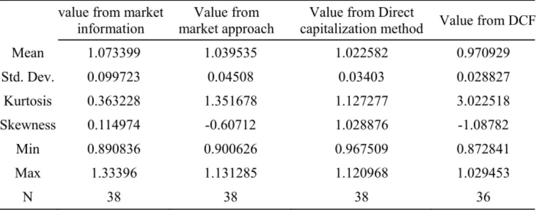
This paper emphasizes the use of disaggregated data to test appraisal smoothing. There are 8 REITs cases in Taiwan. According to the Taiwan Real Estate Securitization Act, trust properties should be reappraised every three months. If there are more than two appraisal values from different appraisal firms, the average real price is the appraisal value. There are 26 real estate reappraisal cases in these 8 REITs. The first one is FuBan number 1 which was issued in the end of 2005 and the reappraisal in 2006Q1. The last day of a season is the reappraisal date. Our data set is panel data. Since the first T-REIT, real estate is a growing market and does not have many decreasing prices . There are 120 reappraisal samples and we obtained 38. The description is in Table 2. From the dispersion degree, the standard deviation of market value, 0.099723, is higher than the other three methods. It indicates that market information is relatively dispersed, implying a valuation smoothing phenomenon.
Table 1. T‐REITs Market (by 2009 October)
Names of REIT Date Issued Trust Property Location Scale(US$ millions)
FuBon REIT#1 Mar. 2005 2 offices, 1Serviced Apartments,1 retail Taipei 241.49
Cathay REIT#1 Oct. 2005 1 office, 1 Hotel, 1 retail Taipei 415.82
Shin Kong REIT#1 Dec. 2005 2 offices, 1 retail, 2 apartments. Taipei, Tainan 447.76
FuBon REIT#2 Apr. 2006 3 offices Taipei 217.91
San Ding REIT Jun. 2006 1 office, 1 retail, 1 warehouse Taipei, Taoyuan 114.93
Kee Tai REIT Aug. 2006 1 office, 1hotel and office Taipei 73.73
Cathay REIT#2 Oct. 2006 3 offices Taipei 214.93
Gallop REIT#1 May 2007 2 offices, 1 warehouse Taipei 127.76
Total volume 26 1743.88
Table 2 Statistic description of market value and appraised value
value from market information
Value from market approach
Value from Direct
capitalization method Value from DCF
Mean 1.073399 1.039535 1.022582 0.970929 Std. Dev. 0.099723 0.04508 0.03403 0.028827 Kurtosis 0.363228 1.351678 1.127277 3.022518 Skewness 0.114974 -0.60712 1.028876 -1.08782 Min 0.890836 0.900626 0.967509 0.872841 Max 1.33396 1.131285 1.120968 1.029453 N 38 38 38 36
3.2 Appraiser’s reappraisal strategy
Following the specification in Equation (5), we can test the null hypothesis by estimating the simple linear regression model.
t j M t j t j t j P P P 2 , , * 1 , 1 0 * , = α +β − +β +ε ………...………(6)
Where dependent variable
* ,t
j
P is the appraised value of property j at time t. Independent
variable includes * 1 ,t− j P and PjM,t . * 1 ,t− j
P is the appraised value of property j at time t-1,
namely previous value.
M t j
P, is a proxy market value variable of property j estimated by
t i t i M t CAP RENT NOI P = ×(1+Δ −) ………(7) Where NOI is net operation income at time i, i ΔRENTt−iis the rent difference between
time i and time t, CAP is the mean value of capitalization rate at time t. t
To reduce variance heterogeneity problems caused by large scale, this study will take the natural logarithm on each variables, and thereby avoid coefficient estimates bias. The double−log model is:
t j M t j t j t j Ln P Ln P P Ln 2 , , * 1 , 1 0 * , ) ( ) ( ) ( =α +β − +β +ε ………..……(8) 4. Empirical Result
4.1 Reaction on market information
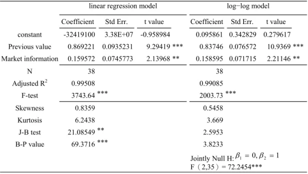
Table 3 presents the result of our test of the smoothing hypothesis in the T-REITs re-appraisal database. It shows in both coefficient estimates that there is not much difference between thetwo models equipped with appropriate well-adjusted R square, 0.99. However both Jarque-bera test and Breusch-Pagan chi-square test indicate that we can reject the null hypotheses, and from lower J-B value we find a linear model can’t fit the requirement of normality and variance heterogeneity. Therefore we used the double log model for continuing analysis.
As table 3 shows, we can reject the null hypothesis at a 1% significance level. There exists in the data partial adjustment behavior. Appraisers give higher weight, 0.83746, for the market information, and less weight, 0.158595, for previous appraised value. This is similar to the result Clayton et al. (2001) did (see table 4).
linear regression model log−log model
Coefficient Std Err. t value Coefficient Std Err. t value
constant -32419100 3.38E+07 -0.958984 0.095861 0.342829 0.279617 Previous value 0.869221 0.0935231 9.29419 *** 0.83746 0.076572 10.9369 *** Market information 0.159572 0.0745773 2.13968 ** 0.158595 0.071715 2.21146 ** N 38 38 Adjusted R2 0.99508 0.99085 F-test 3743.64 *** 2003.73 *** Skewness 0.8359 0.5458 Kurtosis 6.2438 3.669 J-B test 21.08549 ** 2.5953 B-P value 69.3716 *** 3.8233 Jointly Null H:β1 = 0,β2 =1 F(2,35)= 72.2454*** *** Significant at the 1% level.
** Significant at the 5% level.
Table 4 Comparison of appraiser’s confidence on market information
method Reference point Confidence
level,K Familiar the market with
Hansz(2004) Control
experiment
Past transaction
value(higher one) 0.48 Not familiar
Diaz & Hansz(1997) Control experiment Other appraiser’s estimate 0.54 Not familiar
Hansz(2004) Control
experiment
Past transaction
value(lower one) 0.66 Not familiar
Clayton, Geltner, and
Hamilton(2001) Empirical Past appraisal value 0.69 Familiar
Diaz & Wolverton(1998) Control experiment Past appraisal value 0.70 Not familiar
This paper Empirical Past appraisal value 0.86 Familiar
Clayton, Geltner, and Hamilton(2001)
Empirical
Diaz(1997) Control
experiment Past appraisal value 0.88 Familiar
Source:Hansz(2004)
4.2 Reaction on information quality
In this section we will investigate adjustment influence factors. Firstly, we test the rational behavior of appraisers reacting to low quality information. We replace the “noise” proxy variable with the difference rate of market-extracted values. As the value information extracted from the market has greater variation, the appraiser will take insufficient comparatives and know less about the market, or need to place far more adjustment magnitude on property characteristics. Secondly, the type of reference point may have a different impact on the appraiser's level of conservatism; appraisers could have more confidence in their own appraised value rather than in others' valuations. Finally we investigate whether the client background will affect the adjustment pattern, a hypothesis that the size of clients will affect the adjustment parameters will be tested. From equation (4), we rewrite Quan-Quigley model to be equation (9). That is, appraisers will partial adjust to the market change, the difference of contemporaneous market information and last appraised value.
[
*]
1 , , * 1 , * , = − + − jt− M t j t j t j P K P P P …….………...……(9) then , *, 1 * 1 , * , , − − − − = t j M t j t j t j t j P P P P KThe parameter K is what we concern the weight of appraiser put on market information. To avoid K parameter to be zero and not to set aside the unchanged value, we define the dependent variable to be level of conservatism or named anchoring degree (AD), 1-K. The adjustment influence factors model is specified as follow:
ε β α ⋅ + + =
∑
= l n l lD noise AD 1 ……….…………..(10)Noise is defined as the absolute value of the ratio of the difference between comparison value and capitalization value to the comparison value, comps
cap comps P P P noise= − . Higher difference between comparison value and the capitalization value means more noise in the market. A dummy variable set is to test whether reference point and client size affects the adjustment. The variable description is in Table 5.
Table 6 shows that the regression model is significant at 1% level. T-REITs appraisers do react conservatively to low market information as noise increases. The result is the same with Clayton et al. (2001). The dummy set of reference point types shows appraisers refer to transaction prices but not other appraiser’s opinion. Appraisers have less anchoring effect to transaction prices, which means that appraisers have more confidence in their own judgment. Moreover, the model result shows the larger the client is, the more conservative the adjustment strategy.
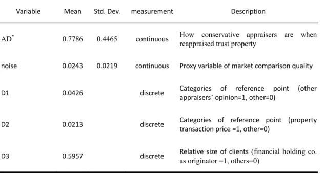
Table 5. Variable description
Variable Mean Std. Dev. measurement Description
AD* 0.7786 0.4465 continuous How conservative appraisers are when
reappraised trust property
noise 0.0243 0.0219 continuous Proxy variable of market comparison quality
D1 0.0426 discrete Categories of reference point (other
appraisers’ opinion=1, other=0)
D2 0.0213 discrete Categories of reference point (property transaction price =1, other=0)
D3 0.5957 discrete Relative size of clients (financial holding co.
* Notes as dependent variable. Table 6. Results of α β ε + + ⋅ =
∑
= i n i iD noise AD 1Variable. Coefficient Std. Err. T-value
noise 8.772 *** 2.680 3.273
D1 -.029 0.339 -0.084
D2 -1.064 ** 0.470 -2.262
D3 .539 *** 0.118 4.572
R-squared = 0.702 Adjusted R-squared = 0.493
F(4,90)= 21.883 Prob.= 0.00000***
***Significant at 1% level. ** Significant at 5% level.
4. Conclusion
Regression results show that we reject the jointly null hypothesis of full adjustment to market fluctuations and the confidence parameter is 0.84. We find that appraisers have partial adjustment strategies. Moreover, we find appraisers give less weight to current market information because of market noise. Noise does decrease appraisers’ confidence. That means appraiser’s partial adjustment is a rational behavior in T-REIT’s reappraisal. The result is similar to Quan and Quigley (1991).
Reference
1. Akerlof, G. A. and R. J. Shiller , 2009, Animal Spirits—How Human Psychology Drives the Economy, and Why It Matters for Global Capitalism, Princeton University Press.
2. Brown, G. R., and G. A. Matysiak, 1998, “Valuation Smoothing without Temporal Aggregation”, Journal of Property Research, 15(2):89-103.
Property Valuation: Evidence from Individual Appraisals”, Real Estate Economics, 29(3) 337-360.
4. Diaz, J., 1997, “An Investigation into the Impact of Previous Expert Value Estimate on Appraisal Judgment”, Journal of Real Estate Research, 13(1):57-66.
5. Diaz, J. and J. A. Hansz, 1997, “How Valuers Use the Value Opinions of Others”, Journal of Property Valuation and Investment, 15(3):256-260.
6. Diaz, J. and M. Wolverton, 1998, “A Longitudinal Examination of the Appraisal Smoothing Hypothesis”, Real Estate Economics, 26(2):349-358.
7. Fisher, J., M. Miles, and R. Webb, 1999, “How Reliable are Commercial Property Appraisals? Another Look”, Real Estate Finance, 16(3):9-15.
8. Geltner, D., 1989a, “Bias in Appraisal-Based Returns”, Journal of the American Real Estate and Urban Economics Association (AREUEA Journal), 17(3): 338–352. 9. Geltner, D., 1989b, “Estimating Real Estate’s Systematic Risk from Aggregate Level
Appraisal-Based Returns”, Journal of the American Real Estate and Urban Economics Association, 17(4): 463–81.
10. Geltner, D., 1991, “Smoothing in Appraisal-Based Returns”, Journal of Real Estate
Finance and Economics, 4:327-345.
11. Geltner, D., 1998, “Appraisal Smoothing: The Other Side of the Story—A Comment”, Available at SSRN: http://ssrn.com/abstract=131459, Working Paper, Department of Finance, University of Cincinnati.
12. Hansz, J. A., 2004, “Prior Transaction Price Induced Smoothing: Testing and Calibrating the Quan-Quigley Model at the Disaggregate Level”, Journal of Property Research, 21(4):321-336.
13. Ibbotson, R., and L. B. Siegel, 1984, “Real Estate Return: a Comparison with Other Investment”, AREUEA, 12:219-242.
14. Kahneman, D. and A. Tversky, 1973, “On the Psychology of Prediction”, Psychological Review, 80(4):237-251.
15. Lai, T.Y., and K. Wang, 1998, “Appraisal Smoothing: The Other Side of Story”, Real Estate Economics, 26(3): 511-535.
behaviour and appraisal smoothing: some qualitative and quantitative evidence”, Journal of Property Research, 20(3):261-280.
17. Quan, D. C., and J. M. Quigley, 1991, “Price Formation and the Appraisal Function in Real Estate Markets”, Journal of Real Estate Finance and Economics, 4: 127-146. 18. Ross, S., and R. Zisler, 1987, “Managing Real Estate Portfolio, Part 3: A Close look
at Equity Real Estate Risk”, Goldman Sachs Real Estate Research, November. 19. Yiu, C. Y., B. S. Tang, Y. H. Chiang, and L. H. Choy, 2006, “Alternative Theories of
98 年度專題研究計畫研究成果彙整表
計畫主持人:陳奉瑤 計畫編號: 98-2410-H-004-132-計畫名稱:不動產估價師部分調整行為之研究 量化 成果項目 實際已達成 數(被接受 或已發表) 預期總達成 數(含實際已 達成數) 本計畫實 際貢獻百 分比 單位 備 註 ( 質 化 說 明:如 數 個 計 畫 共 同 成 果、成 果 列 為 該 期 刊 之 封 面 故 事 ... 等) 期刊論文 0 1 100% 研究報告/技術報告 0 0 100% 研討會論文 0 0 100% 篇 論文著作 專書 0 0 100% 申請中件數 0 0 100% 專利 已獲得件數 0 0 100% 件 件數 0 0 100% 件 技術移轉 權利金 0 0 100% 千元 碩士生 2 2 100% 博士生 0 0 100% 博士後研究員 0 0 100% 國內 參與計畫人力 (本國籍) 專任助理 0 0 100% 人次 期刊論文 0 0 100% 研究報告/技術報告 0 0 100% 研討會論文 2 2 100% 篇 論文著作 專書 0 0 100% 章/本 申請中件數 0 0 100% 專利 已獲得件數 0 0 100% 件 件數 0 0 100% 件 技術移轉 權利金 0 0 100% 千元 碩士生 0 0 100% 博士生 0 0 100% 博士後研究員 0 0 100% 國外 參與計畫人力 (外國籍) 專任助理 0 0 100% 人次其他成果