針對通用圖形處理器上設計模糊類神經網路之架構導向執行緒配對方法

國

立

交

通

大

學

電子工程學系 電子研究所

碩 士 論 文

針對通用圖形處理器上設計模糊類神經網路之架構

導向執行緒配對方法

An Architecture-Aware Thread Mapping

Method-ology for Fuzzy Neural Networks on GPGPUs

研 究 生：曾浩原

指導教授：周景揚 教授

針對通用圖形處理器上設計模糊類神經網路之架構

導向執行緒配對方法

An Architecture-Aware Thread Mapping

Methodology for Fuzzy Neural Networks on

GPGPUs

研 究 生：曾浩原 Student：Hao-Yuan Tseng

指導教授

：周景揚 博士 Advisor：Dr. Jing-Yang Jou

國

立 交 通 大 學

電子工程學系

電子研究所

碩

士 論 文

A Thesis

Submitted to Department of Electronics Engineering and Institute of Electronics

College of Electrical and Computer Engineering National Chiao Tung University In Partial Fulfillment of the Requirements

for the Degree of Master of Science

in

Electronics Engineering September 2012

Hsinchu, Taiwan, Republic of China

I

針對通用圖形處理器上設計模糊類神經網路之架構導向執

行緒配對方法

學生：曾浩原

指導教授：周景揚博士

國立交通大學

電子工程學系

電子研究所碩士班

摘 要

II

An Architecture-Aware Thread Mapping Methodology for

Fuzzy Neural Networks on GPGPUs

Student：Hao-Yuan Tseng

Advisor：Dr. Jing-Yang Jou

Department of Electronics Engineering

Institute of Electronics

National Chiao Tung University

ABSTRACT

The fuzzy neural network (FNN) is extensively used in machine learning applications,

such as classifications. It uses structure and parameter learning phases to create a network

according to the correlation between input training samples and network outputs. Since the

learning phases are getting more time consuming when number of input attributes of training

samples increases, some parallel FNN designs are proposed to speed up the learning

procedure. While designing an efficient parallel FNN, the thread mapping and the architecture

scalability should be taken into consideration to achieve efficient hardware utilization. In this

thesis, we present a parallel FNN design flow including architecture-aware thread mapping

(ATM) methodology. The proposed ATM efficiently utilizes the hardware resource on

GPGPUs by finding a good thread mapping using different training samples and architectures

with different characteristics. The experimental results show that our approach can achieve

III

Acknowledgements

I greatly appreciate my advisors Dr. Jing-Yang Jou. Not only did he made many beneficial

suggestions for me but also provide a resource-intensive environment. I am also really

thankful to Dr. Bo-Cheng Lai for his guidance, valuable suggestions, and encouragement

during these years. I would like to thank Hsien-Kai Kuo for his discussion and help on my

research. Specially thank to all member of EDA Lab for their friendship and company. Finally,

I would like to express my sincerely acknowledgements to my family and my friends for their

IV

Contents

1.2 Fuzzy Neural Network ... 2

1.3 Parallel FNN ... 4

1.4 Thesis Organization ... 5

Chapter 2 Background & Preliminary ... 6

2.1 GPGPU Computing ... 6

2.1.1 Fermi Architecture ... 7

2.1.2 CUDA Programming Model ... 8

2.2 The Self-Constructing Neural Fuzzy Network (SONFIN) ... 10

2.3 Related Work ... 13

2.4 Motivation ... 15

Chapter 3 Our Proposed Approach ... 17

3.1 Bottleneck Analysis……….18

3.2 GPGPU Partitioning……… 20

3.3 Fine-Grain Task Decomposition………... 22

3.4 Special Function Transformation & Memory Coalescing……… 23

3.5 Task Coarsening………...25

3.6 Task to Thread Binding……….. 29

Chapter 4 Experimental Results ... 31

4.1 Experiment Environment...31

4.2 Comparison between Different Optimizations……….…...33

4.3 Discussion of Input Scalability………34

4.4 Discussion of Architecture scalability……….41

4.5 Total Runtime.……….42

Chapter 5 Conclusions & Future Works ... 44

V

List of Tables

Table I Kernel time with different number of rules……….35 Table II Kernel time of different number of dim………..38

VI

List of Figures

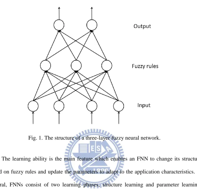
Fig. 1 The structure of a three-layer fuzzy neural network.………3

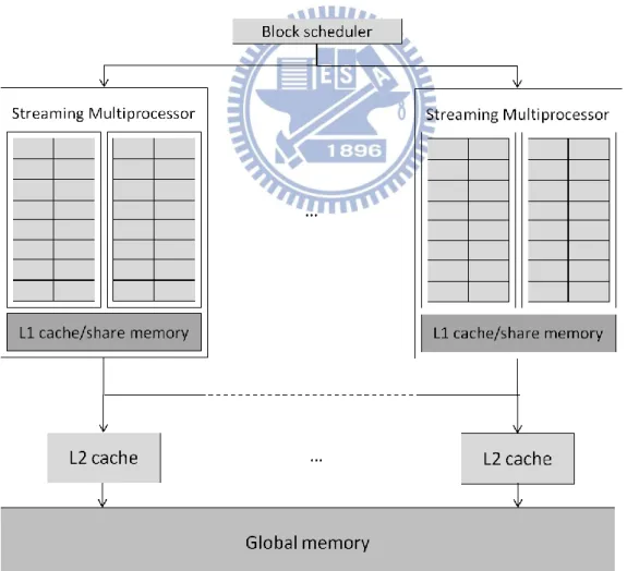
Fig. 2NVIDIA Fermi architecture.…………..………...………...6

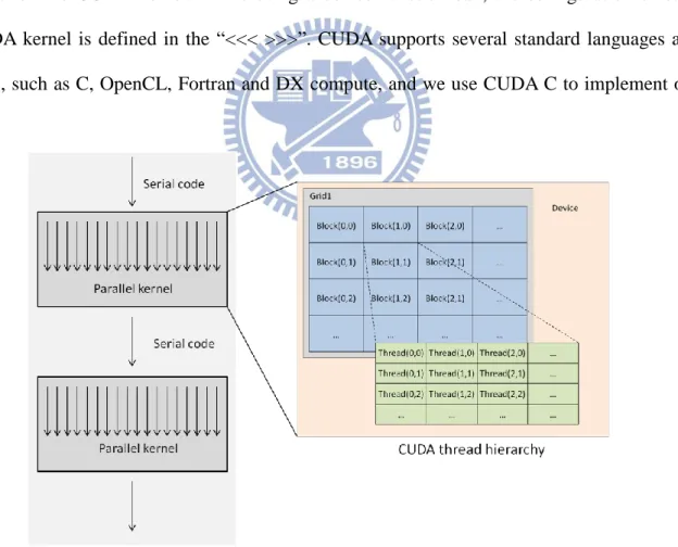
Fig. 3 CUDA programming model..………..8

Fig. 4 Device code and device function call...9

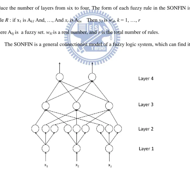
Fig. 5 Modified structure of the SONFIN. ………..……….10

Fig. 6Flow chart of the SONFIN……….12

Fig. 7Design flow of a parallel SONFIN on a GPGPU………...18

Fig. 8Flow chart of the SONFIN……….19

Fig. 9Pseudo code of (a) gaussian member function and (b) update parameter………...20

Fig. 10GPGPU partitioning of the SONFIN………...21

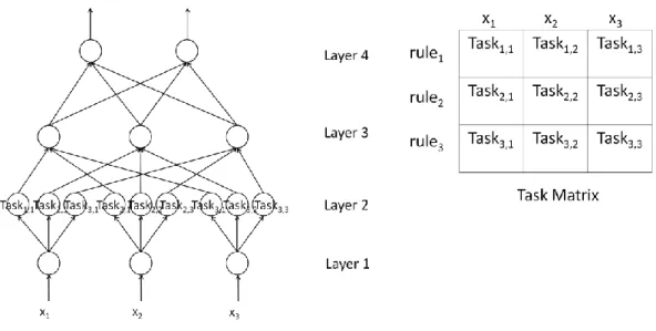
Fig. 11Task Matrix of the SONFIN with 3 dim and 3 rules………22

Fig. 12Coalesced memory access. (a) non-coalesced memory access. (b) coalesced memory access.………...24

Fig. 13Data layout of parallel SONFIN………24

Fig. 14 Task coarsening. ………25

Fig. 15 Two schemes of task coarsening. (a) column-based coarsening. (b) row-based coarsening.………..27

Fig. 16 TM’ to TH binding……….30

Fig. 17 Timing distribution for parallel SONFIN………...30

Fig. 18 Kernel time comparison between each optimizations………32

Fig. 19 Kernel time comparison between GPU-FNN and our approach……….36

Fig. 20 Kernel time trend of different number of rules……….39

VII

1

Chapter 1

Introduction

1.1 Machine Learning

Machine learning is a popular technique over the past two decades, and it is applied to

many applications including weather forecast and image recognition. And many researchers

think it is the best way progress towards human-level AI (artificial intelligence). Machine

learning is so pervasive today that you probably use it many times a day without knowing it.

The most important feature of machine learning is the generalization, which lets a machine

learning algorithm be able to perform accurately on new, unseen examples after training on a

data set. And this feature makes machine learning so powerful and popular. Along with the

increasing requirement of machine automation, machine learning will be widely used in

human’s daily life. Therefore, due to the potential of development of machine learning, many

approaches of machine learning have been proposed in the two decades: decision tree learning,

association rule learning, artificial neural networks, genetic programming and fuzzy neural

network. In this thesis, the fuzzy neural network is used because it takes advantages of

artificial neural network which employs the concept of neural network and fuzzy logic system

2

1.2 Fuzzy Neural Network

Fuzzy neural networks (FNNs) have been applied in many areas including classification

[1] and pattern recognition and so on. A fuzzy neural network is a hybrid system which

combines the features of artificial neural networks (ANNs) and fuzzy logic systems (FLSs).

These two techniques have particular computational properties including advantages and

disadvantages. For example, ANNs are good at recognizing patterns, but they are not good at

specifying the source cause of the decisions. On the contrary, FLSs are good at identifying the

source behind the decisions using fuzzy if-then rules, but they cannot automatically generate

the rules. Furthermore, a fuzzy logic system consists of lots of fuzzy rules, but it is difficult

for human to find the proper number of rules which are related to a great deal of training

samples and network outputs of a complex system. A fuzzy neural network (FNN) is then

emerged to break these limitations. An FNN contains the advantages of an ANN and a FLS,

such as learning ability, easy generalization, fault tolerance and flexibility.

The major learning structures of FNNs can be represented as a three-layer learning

structure. During the learning process, a set of training samples are passed though the three

learning layers as shown in Fig. 1. The first layer corresponds to fetch the training samples

and perform the corresponding pre-procedures. The second layer performs the fuzzy logic

according to a set of fuzzy rules. Finally, the third layer generates the output results. However,

the implementation of each layer can be extended to several layers based on the concept of the

three-layer FNN structure. Note that every training sample has many attributes, and we use

3

The learning ability is the main feature which enables an FNN to change its structure

based on fuzzy rules and update the parameters to adapt to the application characteristics. In

general, FNNs consist of two learning phases, structure learning and parameter learning.

Structure learning modifies the FNN structure to build the correlation of training samples and

fuzzy rules, while the parameter learning tunes the parameters within the network to provide a

more accurate model. Many variations of FNNs have been proposed during the past two

decades [2] ~[16]. However, most of the FNNs focus mainly on building an accurate network

model while putting the runtime of learning as low priority in the tradeoff between accuracy

and learning time. The long learning phases are fine if they are performed off-line. However,

it becomes a serious concern for applications that demand fast learning and model

development, such as stock prediction and weather forecast. These applications require not

only a high quality network model, but also fast learning phases. To address this issue, the

Self-Constructing Neural Fuzzy Inference Network (SONFIN) was proposed in 1998 [3]. Fig. 1. The structure of a three-layer fuzzy neural network.

4

Different from most conventional FNNs, the SONFIN is designed to be an on-line

self-constructing neural inference network. The SONFIN is a general connectionist model of a

fuzzy logic system, which can find its optimal structure and parameters automatically. The

conventional FNNs perform the structure leaning and the parameter learning sequentially. The

substantial runtime makes FNNs with sequential learning scheme only suitable for off-line

operations. Nevertheless, the SONFIN does the structure learning and the parameter learning

simultaneously so that the SONFIN is suitable for fast on-line learning. Moreover, because

the conventional way of grid type partition [2] of the input space increases the number of

rules exponentially with the dim. The SONFIN uses the clustering type partition of the input

spaces which can reduce the number of generated fuzzy rules compared to the grid type

partition.

1.3 Parallel FNN

To construct a more accurate model, users would try to increase the number of fuzzy

rules. This approach could significantly aggravate the runtime of learning phases. It may take

several days to train an FNN with a large number of rules and high dim on a high performance

Central Processing Unit (CPU). For example, it takes more than one day to train a widely

used FNN, ANFIS(an adaptive-network-based fuzzy inference system) with 81 rules on a

CPU with Mackey-Glass test bench [5]. Fortunately, due to the nature of a distributed network,

FNNs are usually inherent massive computing parallelism. This feature makes an FNN

suitable to be implemented on many-core systems. In fact, parallel computing has been

proved to be effective to reduce the training time during the learning phases. The

experimental results of GPU-FNN [17] showed up to 78.51x speedup on a handwritten

5

1.4 Thesis Organization

The rests of this thesis are organized as follow. Chapter 2 introduces the background of

FNNs which is used in this thesis. The proposed methodology is introduced in chapter 3.

Chapter 4 shows our experimental results and chapter 5 concludes the contribution of this

6

Chapter 2

Background & Preliminary

This chapter introduces the background and motivation of this work. Section 2.1

introduces the GPGPU computing platform, NVIDIA Fermi architecture and its programming

environment CUDA. Section 2.2 introduces SONFIN, which is a classical type of FNN and

widely used in many domains.

2.1 GPU Computing

7

Graphic Processing Unit (GPU) is originally designed for computer graphics only. The

computations in graphic based applications are often independent, massive and regular. Hence,

the designs of GPUs architecture always focus on computations. On the other hand, the CPU

needs to handle more complicated controls. So the major difference between CPU and GPU is

that, GPU issues a lot of simple processing elements but CPU consists of few complex

processing units. However, due to the increasing complexity of general applications, the

runtime of CPU is getting longer. For this reason, GPU has been applied to various algorithms

in many areas, and this kind of GPU is called general purpose GPU (GPGPU).

2.1.1 Fermi Architecture

NVIDIA is one of the companies that focus on the design of GPGPU. An architecture

announced by NVIDIA Corporation [18] is named Fermi. The Fermi architecture is a

single-instruction-multiple-thread (SIMT) system as shown in Fig. 2; it contains several streaming

multiprocessors (SMs). At the same time, all the SMs can share a unified L2 Cache and

DRAM. There are 32 cores, four special function units and a 64KB local memory which is

only shared among all the CUDA cores in a SM. Each of these cores can be launched in

parallel with a huge amount of threads. For example, NVIDIA Tesla C2050 can launch up to

1536 threads per SM. Meanwhile, NVIDIA provides programmers with the CUDA

programming Model [19] so that the programmers can control thousands of threads on the

8

2.1.2 CUDA Programming Model

CUDA is a parallel programming model that can be run on any number of processors

without recompiling. As shown in Fig. 3, parallel portions of an application are executed on

the device as CUDA kernels. In a CUDA kernel, programmers have to define the CUDA

thread hierarchy. The right hand side of Fig. 3 shows the CUDA thread hierarchy which

contains three levels, grid, block and thread. A CUDA kernel is executed by an array of

threads, and all the threads run the same code. Each thread has its own ID that is used to

compute memory addresses and make control decisions. Fig. 4 shows an example of device

code which is executed in every thread, and the device function call which is used in the main

to launch the CUDA kernel. While using a device function call, the configuration of each

CUDA kernel is defined in the “<<< >>>”. CUDA supports several standard languages and

APIs, such as C, OpenCL, Fortran and DX compute, and we use CUDA C to implement our

9

program in this thesis. And CUDA is supported on common operation system, such as

Windows, Mac OS and Linux.

During the execution of a CUDA kernel, block scheduler issues several thread blocks to

each SM, and each SM further divides thread blocks into warps, which consist of 32 threads,

to carry out a fully parallel execution on the cores. In the Fermi architecture, there are several

restrictions on the maximum number of blocks, warps and threads on each SM which are

different with different computing capability. For example, on a NVIDIA Tesla C2050 graphic

card, the maximum number of thread blocks, warps and threads are 8, 48 and 1533

respectively.

According to the official CUDA programming guide [20], occupancy shows how

effective the hardware is kept busy. It is a ratio of active warps to limit warps which is the

maximum number of warps on a SM. The definition of occupancy is

When defining the CUDA thread hierarchy, the size of thread blocks highly influences the Fig. 4. Device code and device function call.

10

occupancy. For example, limit warps is 48, maximum number of thread blocks is 8, block size

is 32, than there will be 8 thread blocks and 8 warps issued on a SM, so the occupancy is

0.0667. Another example, limit warps is 48, block size is 192, than there will be 8 blocks and

48 warps issued on a SM, so the occupancy is 1. Although higher occupancy does not always

equate to higher performance, low occupancy always interferes with the ability to hide

memory latency, resulting in performance degradation [21].

2.2 The self-constructing neural fuzzy network (SONFIN)

Fig. 5 shows the modified structure of the SONFIN. The original SONFIN structure has

six layers. In order to make the comparison between serial and parallel version easier, we

reduce the number of layers from six to four. The form of each fuzzy rule in the SONFIN is:

Rule R : if x1 is Ak1 And, …, And xr is Akn Then y1 is wrl, k = 1, …, r

where Akj is a fuzzy set. wkl is a real number, and r is the total number of rules.

The SONFIN is a general connectionist model of a fuzzy logic system, which can find its

11

optimal structure and parameters automatically. The function of each layer is described below.

Layer 1:

One node corresponds to one dim. No computation is done in this layer, and each

node transmits input values to the next layer.

Layer 2:

Each node corresponds to one fuzzy set and calculates a membership value. That is,

the membership value which specifies the degree to which input value belongs a fuzzy set

is calculated in this layer. The fuzzy set Akj is employed with the Gaussian membership

function:

where mrj is the center of the fuzzy set and the denotes the width of the fuzzy set. So

the number of fuzzy sets in each dim is equal to the number of fuzzy rules.

Layer 3:

A node in this layer represents one fuzzy rule and performs antecedent matching of a

rule. The following AND operation is performed for each node in layer 3:

where X = [x1, … , xdim]. The number of fuzzy nodes in this layer is equal to the number

of rules.

Layer 4:

This layer contains many output nodes, and the number of output nodes is equal to the

number of output dimension. Each output node performs as a defuzzifier by using a

12

where L is the number of output dimension.

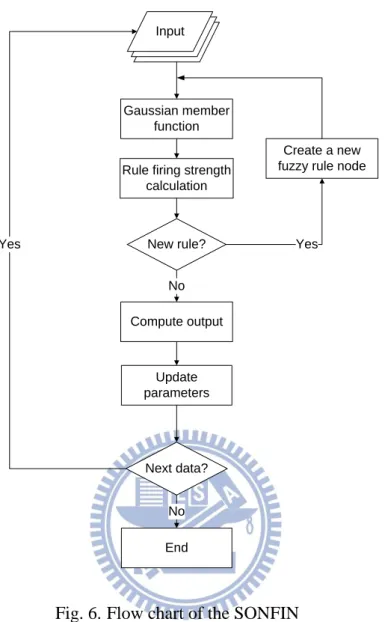
Fig. 6 shows the flow chart of the SONFIN. The flow chart includes the structure learning

and parameter learning. In the structure learning, there are no rules initially, and rules are

constructed by the structure learning. The firing strength in layer 3 is used to decide whether a new fuzzy rule is generated. If , a new rule

is generated, where the is a prespecified threshold that decays with training iteration number. If a new rule is generated, the center and width of corresponding membership

functions are: Input Gaussian member function New rule? Update parameters Next data? Rule firing strength

calculation

Compute output

Create a new fuzzy rule node

No End

Yes Yes No

13

where is a coefficient which determines the overlapping between two rules in the input space.

The parameter learning tunes all the parameters by using a gradient descent algorithm.

The parameters are updated using the equation below:

where is a learning constant which influences the converging speed of the gradient decent algorithm.

2.3 Related Work

FNNs have been studied for decades, and many FNNs with different propertied have

been proposed. ANFIS (Adaptive Neuro-Fuzzy Inference Systems) was proposed in 1993 [2].

It is a widely used FNN which only performs parameter learning. ANFIS uses a hybrid

learning procedure to build the connection between training samples and network output

based on both human knowledge and stipulated input-output data pairs. However, the number

of fuzzy rules of FNNs with only parameter learning increases exponentially with the

14

to reduce the number of generated rules.

Recently, there are some researches focusing on parallel neural networks [22][23] and

parallel fuzzy neural networks [17][24]. [22] implemented the parallel neural network by

mapping the inner-product operation into a matrix multiplication operation. [23] provided an

implementation of the back-propagation algorithm on CUDA, and the author claimed that the

number of threads should be as large as possible to enable the CUDA scheduler to better

utilize the available computational power. The first adaptation of the Fuzzy ARTMAP neural

network on a GPGPU was proposed in [24]. Juang and Chen [17] proposed an

implementation of a zero order Takagi-Sugeno-Kang-type fuzzy neural network on GPU. To

our best knowledge, Juang is the first work which gives a detailed SONFIN design on a

GPGPU. This paper uses this work as the baseline design to compare the experimental results.

However, the performance of a parallel application on the GPGPU heavily depends on

how the developer manages blocks of threads and how effective the GPGPU hardware

resource is used. The thread mapping in NVIDIA CUDA kernel determines how much

parallelism can be exploited by a GPGPU. The thread mapping of the GPU-FNN [17] was

partitioned based on fuzzy rules. In this way, each fuzzy rule in a FNN is mapped on a thread

block. GPU-FNN can make good use of the parallel fuzzy rules in some cases, for example,

192~768 dim with NVIDAI Tesla C2050. However, the range of dim of different applications

can vary significantly. For example, an artificial detection might have tens of dim [25], while

the protein mutant data set could involve more than five thousand dim [26]. The design of a

parallel FNN needs to cover all the possible range of dim from different applications.

Moreover, the current version of CUDA programming model limits a thread block to

accommodate up to 1,024 threads. Therefore, the mapping method proposed in [17] cannot

15

2.4 Motivation

With the approaches of [22] and [24], the efficiency of the hardware utilization is not

considered. The author of [23] claimed that the number of threads should be as large as

possible to enable the CUDA scheduler to better utilize the available computational power.

However, this approach does not take how effective the threads could exploit the GPGPU

architecture into account. In the [17], blocks of threads are partitioned based on fuzzy rules so

thatthe hardware is not efficiently used with some training samples. In summary, the thread

mapping mechanism of these works cannot adapt to training samples with different

characteristics and architecture with different features.

The performance of a parallel application on a GPGPU is highly dependent on how

effective the created threads could exploit the GPGPU architecture. The decisive factor is the

thread mapping mechanism, which connects a multi-thread application to the underlying

many-core system. This becomes a non-trivial problem when implementing an FNN onto a

GPGPU. The main design concerns can be characterized as follows:

(1) Parallelism and coordination. The way an application is parallelized and how the

concurrent computation is coordinated also plays important roles in the GPGPU computing. A

well parallelized application can reduce the computation burden on GPGPUs and achieve

superior performance enhancement. However, an inappropriate design may ignore important

design issues, such as insufficient parallelism or severe resource contention, and cause

degraded performance.

(2) Thread mapping. Although FNNs have massive computation parallelism, the thread

mapping must be well designed because it could significantly influence the efficiency of

hardware utilization. However, an efficient thread mapping design of a parallel FNN is not

straightforward, it must take many factors into concern, such as compute capability of the

16

(3) Adaptability and scalability. It is predicted that the number of cores in a GPGPU will

scale with the advances of semiconductor technology. The performance of a multi-threaded

FNN should automatically scale with the enormous cores provided by the future GPGPUs

without redesign overhead. Moreover, the design should also be adaptable to the changing

number of fuzzy rules and dim of an FNN.

Because of these design concerns abovementioned, we propose an architecture-aware

thread mapping methodology for FNNs on GPGPUs which can create efficient coordination

between concurrent computations and hardware on GPGPUs based on the training samples

17

Chapter 3

Our Proposed Approach

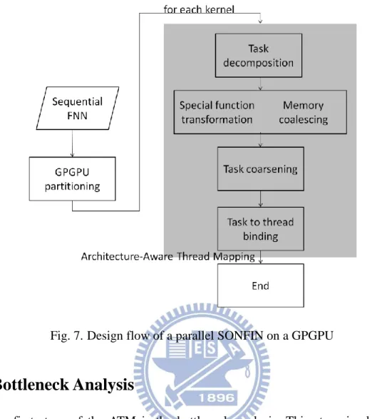
Fig. 7 shows a design flow to parallelize and optimize FNNs on a GPGPU. This thesis

uses the modified SONFIN as the main application to demonstrate the effectiveness of the

proposed design flow. This flow considers several important issues of FNNs using GPGPU

computing. The design flow starts from a sequential FNN application. The first stage shown

in the Fig. 7 is necessary in every parallel design to decide which parts of the program should

be parallelized and executed on GPGPUs. The shaded block on the right hand side of Fig. 7 is

the Architecture-Aware Thread Mapping (ATM). The ATM performs optimizations for each

CUDA kernel, and contains four stages, 1) fine-grain task decomposition, 2) special function

transformation and memory coalescing, 3) task coarsening and 4) task to thread binding. The

18

3.1

Bottleneck Analysis

The first stage of the ATM is the bottleneck analysis. This stage is almost the most

important and essential stage while designing a parallel program. The bottleneck analysis is to

find out bottlenecks that dominate the runtime of the total program. According to Amdahl’s

law, if a fraction f is accelerated by a factor of S, the overall performance speedup is:

In the parallel computing, the is the fraction that can be parallel in a sequential program. And the fraction can be accelerated S times after parallelization. Factor S is decided by how much parallelism of the f part and how well the GPGPU architecture can be exploited. Larger

could increase the impact of S on the overall performance. So it is important to find out which parts have the greatest f through the bottleneck analysis.

19

Because the conformation of an FNN is fixed no matter how many dim and number of

rules. So the easiest and the most efficient way to catch the computation behavior is to profile

the timing information of an FNN with a small bench which has small dim and little number

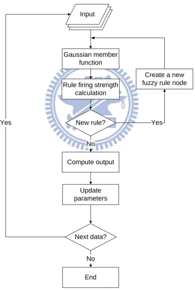
of rules. Fig. 8 shows the flow chart of the SONFIN, and we found two bottlenecks, the

gaussian member function and the update parameter, by bottleneck analysis. And their pseudo

code is shown in Fig. 9. Through our profiler, the gaussian member function takes about 80%

and the update parameter takes about 15% of the total runtime.

Input Gaussian member function New rule? Update parameters Next data? Rule firing strength

calculation

Compute output

Create a new fuzzy rule node

No End

Yes Yes No

20

3.2

GPGPU Partitioning

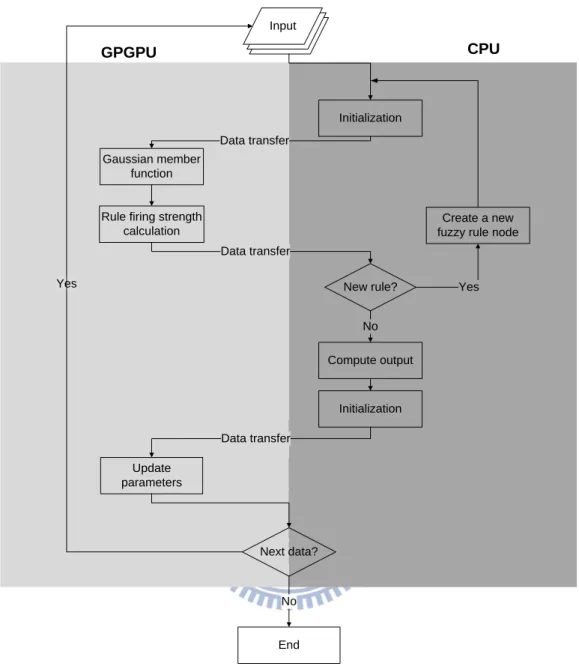
Using the result of bottleneck analysis, we can have a initial partitioning. The gaussian

member function and the update parameter have been recognized as the two bottlenecks that

should be parallelized as CUDA kernels on GPGPU. However, in addition to the execution

time of individual function block, the partitioning of GPGPU and CPU should also consider

issues such as the effectiveness of parallel part of a program and data transfer between a

device and a host. However, we perform the partitioning based on the rule of thumb. Besides

the two bottlenecks of the SONFIN, the rule firing strength calculation is also moved to the

GPGPU in our partitioning. This is because the amount of data transfer between Gaussian

member function and rule firing strength calculation is larger than the amount of data transfer

between rule firing strength calculation and new rule decision. Based on the above analysis,

the final partitioning is shown in Fig. 10. The following subchapter will use this partitioning

scheme to perform optimizations in the ATM methodology.

(a) Gaussian member function (b) update parameter

21 Input Gaussian member function New rule? Update parameters Next data? Rule firing strength

calculation

Data transfer

Compute output

Create a new fuzzy rule node

No End Yes Data transfer Yes No Initialization Data transfer Initialization GPGPU CPU

22

3.3

Fine-Grain Task Decomposition

The first stage of the ATM is decomposition. It defines how the computations executed

simultaneously on the GPGPUs. Recall that the pseudo codes of the two bottlenecks are

shown in Fig. 9, and it can be seen that they have two nested for loop. So in each CUDA

kernel, we use a 2-D matrix, Task Matrix (TM), to represent the overall computation. The

definition of TM is:

Definition 1 (Task Matrix) A Task Matrix is a 2-D matrix which is used to stand for the

overall computation of a CUDA kernel. It is a matrix, where r is total number of rules and dim is total number of input attributes. And each element in a TM is named Task which is defined in the definition 2.

Definition 2 (Task) A task is a computation of one input dimension of one rule. Therefore, Tij is the computation of rule and input attribute pair (i, j). For example, T23 is the computation of the 2th rule to the 3th input attribute.

We decompose the parallelism of each CUDA kernel in the most fine-grained way by

defining the TM and the Tasks. The reason is that the fine-grained decomposition extends the

23

space of configuration of each CUDA kernel. We later use the task coarsening to search the

configuration space of each CUDA kernel. So the configuration with better performance can

be easily found. The searching procedure will be discussed in the section3.5. For the parallel

SONFIN, Fig. 11 shows an example of Task Matrix with 3 dim and 3 rules, and the Task

Matrix is a 3x3 Matrix.

3.4

Special Function Transformation & Memory Coalescing

The second stage of the ATM contains two optimizations, special functions

transformation, and memory coalescing. Because these two optimizations are independent,

they are designed in the same stage, and can be performed simultaneously. The purpose of

special function transformation is to utilize the special function hardware which is faster than

the compiled ptx code to speed up the mathematical operations. The special functions

transformation uses the library supported by CUDA, such as addition, subtraction,

multiplication, division and other mathematical operations. The special functions units are

faster than the standard functions because the special functions directly use the special

function units on the GPGPU. However, the number of special function units on the GPGPU

is limited, so the number of special functions which are changed from standard functions is

limited. This problem is like an simple version bin packing problem, so we can use the first fit

algorithm which is a straightforward approach to select the most effective special function

transformation.

Memory subsystem had been always identified as a crucial bottleneck in the GPGPU

computing. There is an optimization of memory access which is called coalesced memory

coalesced access. The coalesced memory access is a technique to combine multiple data

accesses into one single memory transaction. In an SIMT architecture, the memory access

24

memory transaction. As an example shown in Fig. 12 (a), assume the data which are needed

by the half warp is scattered to memory, so there require total sixteen memory accesses. Fig.

12 (b) illustrates the case that the data needed by the half warp is stored adjacently in the

memory, so all the memory access will be packed into only one memory transaction.

According to the regular data structure of FNN, the memory coalescing can be done by (a) non-coalesced memory access

(b) coalesced memory access

Fig. 12. Coalesced memory access. (a) non-coalesced memory access. (b) coalesced memory

access.

25

designing the data layout. Generally there are two styles of data layout which are used in

regular data, row-wise and column-wise. According to the introduction of memory coalescing

before, as long as the data of adjacent threads are stored in the adjacent memory address, the

memory access is optimized by memory coalescing. However, the number of rules will

change during the learning, so the data layout is limited by the direction of dim. Fig. 13 shows

our data layout of the parallel SONFIN.

3.5

Task Coarsening

The third stage of the ATM is task coarsening. The coarsening is an optimization

technique to fine-tune the parallelism decomposition. Fig. 14 shows the concept of task

coarsening. A single block represents a computation; a task is composed of three common

computations and one unique computation. There are four tasks which are executed

simultaneously, and the amount of total computations is after three time

26

stamps. If we coarsen two tasks into one task, the common computations are just executed

once and stored into registers. So a task becomes a task’ which is consist of three common computations and two unique computations. Therefore, the amount of total computations is

reduced to after the task coarsening. Moreover, because the number of common computations is decreased, so the memory accesses in the common computations are

also decreased. However, there are some overheads to perform task coarsening: the indexing

will cost extra computation in our last stage, task to thread binding.

In summary, there are two benefits of the task coarsening, 1) reduce the total amount of

computation 2) reduce the data access from memory. However, in the task coarsening

optimization we have to decide which tasks should be coarsened together and how many tasks

should be coarsened so that we can strike a balance between parallelism and amount of

computation. We define two schemes to coarsen tasks, column-based coarsening and

row-based coarsening. The row-row-based coarsening coarsens tasks within a rule and the column-based coarsening coarsens tasks in different rules. Fig. 15 (a) shows the column-column-based coarsening. To maintain the memory coalescing, the stripe width should be the number of

thread in a warp. Fig. 15 (b) shows the row-based coarsening. The Task Matrix is transformed

into Task Matrix’ after the task coarsening. We can use one of these two schemes to do the

task coarsening.

TM’= coarsen_column( TM, n)

TM’: Task’i,j = Taski,j ∪ Taski,j+w ∪ Taski,j+2w ∪ …∪ Taski,j+nw , nw < dim

TM’= coarsen_row( TM, n)

TM’: Task’i,j = Taski,j ∪ Taski+p,j ∪ Taski+2p,j ∪ …∪ Taski+np,j , p =

Where n is the coarsen number, and w is the coarsen width. And there is a property to

27

Property: While determining the n, the parallelism should be considered. Therefore, we

assume the hardware on GPGPUs is fully utilized if each core has at least one tasks to execute, that is, , where dim is the total number of input attributes and r is the

number of rules.

(a) column-based coarsening

(b) row-based coarsening

Fig. 15. Two schemes of task coarsening. (a) column-based coarsening. (b) row-based

28

We can know the upper bound of n by the property above, and then we extract each

CUDA kernel in the SONFIN to find the optimal configuration of task coarsening by the

coarsen configuration search which is shown below. The Confcoar is a configuration pair

{ coarsen scheme, coarsen number }, and it decides which coarsen scheme should be used and

how many tasks should be coarsened. The evaluation( C( TM, i ) ) function returns the CUDA

kernel time of a CUDA kernel using the coarsen scheme C with i coarsened tasks. The

coarsen configuration search scans the design space for the two coarsen schemes and for the

reasonable coarsen number, and choices the best one. Then we use the returned coarsen

scheme and coarsen number to perform the tasks coarsening.

Coarsening Configuration Search(Confcoar, TM, n)

1. Confcoar ←

2. best ←

3. for 0<i<n

4. for C←{ coarsen_raw, coarsen_column }

5. if( evaluation( C( TM, i ) ) < best)

6. best ← evaluation( C( TM, i ) )

7. Confcoar ← (C, i)

8. end if

9. end for

10. end for

29

3.6

Task to Thread Binding

The last stage of the ATM is task to thread binding. It creates the connection between the

tasks and the CUDA thread hierarchy. We use a matrix, Thread Hierarchy (TH), to stand for

the thread hierarchy in the CUDA. TH is a matrix, which Nb is the number of thread

block and Nt is the size of a thread blocks. There are three hints to follow to have a good task

to thread binding: First, define the TH with Nt that can make occupancy 100%. There are

many choices of Nt that can make occupancy 100%, however, we chose the smallest one to

avoid the load balancing issue. Second, the task bound within the same block should be

adjacent to maintain memory coalescing. Third, easier computation of the indexing in each

CUDA kernel is better. Based on the three hints, Fig. 16 shows a simple example of our task

to thread mapping. Actually, the tasks to thread binding becomes very easy after the first three

stages of the ATM. We just need to design the Nt which can make occupancy 100%, then map

the TM’ to TH according to the data layout direction. In this way, the hardware on GPGPUs

can be utilized efficiently, and the memory accesses are coalesced; moreover, the

computations are simple to calculate the indexes.

After the ATM, each kernel has been optimized. And then we profile the parallel SONFIN

to get the timing information, which is shown in Fig. 17. We can see how many percentage of

each function block takes in Fig. 17. In the Fig. 10, the gaussian member function originally

takes 85% total runtime, but it takes 25% after parallelization. The update parameter takes

13%, but it takes 4.62% after parallelization. As a result, the original bottlenecks are

accelerated. However, there are three data transfer overhead, they takes 0.015%, 23% and

30

Fig. 16. TM’ to TH binding

31

Chapter 4

Experimental Results

4.1 Experimental Environment

In this thesis, all the experiments are conducted in a workstation with Intel Xeon CPU

E5640, 64 GB RAM. The experiments in section 4.1~4.3 and section 4.5 are evaluated with

the NVIDIA Tesla C2050. And the following four architectures are used in the section 4.4,

NVIDIA GeForce 9800 GT, Tesla C1060, Tesla C2050 and GeForce GTX 680. Note that the

parallelization does not change the original algorithm. Hence, the error rate should be the

32

(a) Kernel time of 32 dim and scaled number of rules

(b) Kernel time of 512 dim and scaled number of rules

(c) Kernel time of 1024 dim and scaled number of rules

Fig. 18. Kernel time comparison between each optimizations

0 10 20 30 40 50 32 128 224 320 416 512 608 704 800 896 992 CUD A k e rn e l t im e ( s) number of rules GPU-FNN C C+Binding 0 50 100 150 200 250 32 128 224 320 416 512 608 704 800 896 992 CU D A k er n el t im e (s) number of rules GPU-FNN C C+Binding 0 100 200 300 400 500 600 700 32 128 224 320 416 512 608 704 800 896 992 CUD A k e rn e l t im e ( s) number of rules GPU-FNN C C+Binding

33

4.2 Comparison Between Different Optimizations

This section discusses the effects of each optimization technique. In this section, we use

NVIDIA Tesla C2050 as the default architecture. And we directly set the dimension and

number of rules to get the kernel time in the experiments in section 4.2~4.4. All the kernel

time is extracted and accumulated to see impacts on each CUDA kernels of each optimization.

Fig. 18 compares the kernel time with fixed dim using two optimizations, task coarsening and

task to thread binding. The term C means task coarsening and the term Bind stand for task to

thread binding. Because the GPU-FNN has done the special function transformation and

memory coalescing, so we just compare these two optimizations.

Fig. 18(a) shows the 32 dim case. The task coarsening gains almost no benefit with any

number of rules. This is because the task coarsening decreases the parallelism. On the other

hand, the task to thread binding significantly decreases the kernel time when the number of

rules is larger than 224. When the number of rule goes to 992, task to thread binding gains up

to 45% performance improvement.

In the case of 512 and 1024 dim in Fig. 18(b)(c), the task coarsening gets about 15%

performance improvement when the number of rules is 992. Because the dim is large enough,

so the parallelism after task coarsening is still large enough for parallel computation. The task

to thread binding delivers a limited improvement in the 512 dim case, because the hardware

utilization rate of GPU-FNN and ours are approaching maximum. But in the case of 1024 dim,

the task to thread binding has up to 20% improvement when the number of rules is 992. The

main reason is because a thread block only supports up to 1024 threads in the CUDA

programming model. Then only one thread block can be issued on a SM, and occupancy of a

SM is 32/48 = 0.6667 by using the GPU-FNN. However, The occupancy is still 100% by

34

4.3 Discussion of Input Scalability

This section discusses the kernel behavior using training samples with different

characteristics. We first fix the dim of training samples and change the number of rules. Table

I shows the kernel time of 32, 512 and 1024 dim with varying number of rules, and Fig. 19

shows the bar charts. The occupancy are 0.1667, 1 and 0.6667 for these three cases

respectively. In the 32 dim case which is shown in Fig. 19(a), our approach cannot gain

benefit when the number of rules is smaller than 224. However, when the number of rules is

larger than 224, our approach starts to have advantage and the advantage is larger when the

number of rules increases. Fig. 19(b) shows the case of 512 dim, but the performance

improvement of our approach is not impressive. This is because the SM occupancy rate of

GPU-FNN is almost 100% in 192~768 dim, so there is no room for us to gain benefit.

Nevertheless, when the dim is fixed to 1024 which is shown in Fig. 19(c), the SM occupancy

rate of GPU-FNN is not 100%. Therefore, our approach can gain improvement from the

occupancy. If the dim is larger than 1024, the GPU-FNN cannot work because a thread block

can only support up to 1024 threads. Our approach can works normally by dynamically

35

36

(a) Kernel time of 32 dim and scaled number of rules

(b) Kernel time of 512 dim and scaled number of rules

(c) Kernel time of 1024 dim and scaled number of rules

Fig. 19. Kernel time comparison between GPU-FNN and our approach

0 10 20 30 40 32 128 224 320 416 512 608 704 800 896 992 CUD A k e rn e l t im e ( u s) number of rules GPU-FNN ours 0 50 100 150 200 250 32 128 224 320 416 512 608 704 800 896 992 CUD A k e rn e l t im e ( u s) number of rules GPU-FNN ours 0 100 200 300 400 500 600 700 32 128 224 320 416 512 608 704 800 896 992 CUD A k e rn e l t im e ( u s) number of rules GPU-FNN ours

37

Besides, we fix the number of rule with varying dim. Table II shows the kernel time of

256, 512, 768 and 1024 rules with varying dim, and Fig. 20 shows the timing charts. Note that

the GPU-FNN cannot work if the dim is larger than 1024. The speedup of our approach is

about 1.5X in these four cases when the dim is 1024. One can find that the kernel time of

GPU-FNN increases extremely when the dim is 768. Because a SM can issue two thread

blocks when the dim is 768. When the dim increased, only one thread block is issued on a SM.

Then the performance degrades because occupancy is decreased. This problem will happen

when 768 1024 in Tesla C2050. However, our approach does not have this issue. It can be seen that the trend of the kernel time of the four cases are similar. It is

reasonable to inference that the percentage of performance improvement is fixed no matter

38

39

(a) Kernel time trend of 256 rule

(b) Kernel time trend of 512 rules

(c) Kernel time trend of 768 rules

(c) Kernel time trend of 1024 rules

Fig. 20. Kernel time trend of different number of rules

0 50 100 150 200 32 96 _{160 224 288 352 416 480 544 608 672 736 800 864 928 992} CUD A k e rn e l t im e (u s) input dimension GPU-FNN ours 0 100 200 300 400 32 96 _{160 224 288 352 416 480 544 608 672 736 800 864 928 992} CUD A k e rn e l tim e (u s) input dimension GPU-FNN ours 0 100 200 300 400 500 32 96 _{160 224 288 352 416 480 544 608 672 736 800 864 928 992} CUD A k e rn e l t im e (u s) input dimension FNN-GPU our 0 200 400 600 800 32 96 _{160 224 288 352 416 480 544 608 672 736 800 864 928 992} CUD A k e rn e l tim e (u s) input dimension GPU-FNN ours

40

(a) Kernel time of 512 dim using Tesla C1060

(b) Kernel time of 512 dim using GeForce 9800 GT

(c) Kernel time of 512 dim using GeForce GTX 680

Fig. 21. Kernel time with three different architectures

0 100 200 300 400 500 600 700 32 128 224 320 416 512 608 704 800 896 992 CUD A k e rn e l t im e ( u s) rule number GPU-FNN our 0 1000 2000 3000 4000 32 128 224 320 416 512 608 704 800 896 992 CUD A k e rn e l t im e ( u s) rule number GPU-FNN our 0 50 100 150 32 128 224 320 416 512 608 704 800 896 992 C UDA ke rn e l t im e ( u s) number of rules GPU-FNN our

41

4.4 Discussion of Architecture Scalability

In this section, we discuss the architecture scalability of our approach using the other

three GPGPU architectures, NVIDIA GeForce 9800 GT, NVIDIA Tesla C1060 and NVIDIA

GeForce GTX680. Note that the GPU-FNN can only support up to 512 dim when using

NVIDIA GeForce 9800 GT and NVIDIA Tesla C1060. Therefore, we show the results of 512

dim which are shown in Fig. 21. Remind that we had experiment for kernel time of 512 dim

with changing number of rules in section4.2 using NVIDIA Tesla C2050, the reduction of

kernel time is up to 16 %. In Fig. 21, largest reduction of kernel time is 28%, 30% and 20%

for 9800GT, C1060 and GTX680 respectively.

To show the scalability of number of cores using our approach, Fig. 22 compares the

kernel time using different graphic cards with 512 dim test bench. Note that the sequence of

number of cores is: GTX680>C2050>C1060>9800GT. As in Fig. 22, it can be seen that the

performance can be further improved by using the GPGPU with more cores, that is saying,

our approach has scalability for number of cores which is the architectural trend in the future.

Fig. 22. Kernel time of our approach using four different architectures

1 10 100 1000 10000 32 128 224 320 416 512 608 704 800 896 992 CUD A k e rn e l t im e ( u s) number of rules 9800 GT C1060 C2050 GTX 680

42

4.5 Total Runtime

Table III shows the comparison of total runtime. In Table III (a), we use random uniform

generated benches, and we generate four benches with different dim. The 32, 256, 1024 and

2048 dim can be used to represent the low, medium, high and very high dim respectively. In

the cases of 32 and 1024 dim, our implementation reduce the total runtime up to 19% when

comparing with the GPU-FNN implementation. The main reason is that GP-FNN cannot

achieve a good hardware utilization of GPGPU in these two cases. But the ATM in our

approach can always control the hardware utilization in a very high level. However, the

performance improvement in the case of 256 dim is only 6%, because the hardware utilization

of GPU-FNN is also really high, so there is no room to gain benefit from the hardware

utilization. The 2048 dim is a special case. In this case, the GPU-FNN cannot handle the very

high dim. However, our approach still works normally, and has 443x speedup over CPU

implementation. Table III (b) shows real cases, and the improvement can be up to 11.96%

with isolet5 bench compared to GPU-FNN. We can notice that the improvements of total

runtime are smaller than the improvements of the kernel time experiments before. The main

reason is the number of rules is increasing from 0, and the parallelism is not large enough to

have massive improvement with small number of rules. As a result, the overall performance

43

Table III Total runtime

(a) Synthetic benches

44

Chapter 5

Conclusions & Future Works

In this thesis, we present a design flow for parallel FNNs on GPGPUs. In the design flow,

we propose the architecture-aware thread mapping (ATM) methodology to optimize each

CUDA kernel. The task decomposition and coarsening scheme scans the design space of a

parallel FNN. By considering different characteristics of FNNs and training samples, the

proposed scheme can find appropriate parallelism which can fully exploit the computing

capability of GPGPUs. Moreover, the task to thread binding maps the high level tasks to the

concurrent threads. This binding methodology concerns not only the architectural features of

GPGPUs, but also the characteristics of FNNs such as dim. The proposed binding

methodology from tasks to thread provides performance scalability with the increasing

number of cores of GPGPUs and changing dim and rules of FNNs.

Experimental results show that the kernel time can be reduced by 20%~40%, and the

reduction of total runtime is up to 20% compared with the GPU-FNN. Compared with the

CPU implementation, the total runtime speedup can be up to 460X. As a result, the proposed

ATM methodology makes it more practical to apply an FNN to solve different problems. And

45

References

[1] Y. Cai and H. K. Kwan, “A fuzzy neural classifier for pattern classification,” in Proc. Int. Symp.

Circuits Systems, Chicago, IL, May 3–6, pp. 2367–2370, 1993.

[2] J. S. Jang, “ANFIS: Adaptive-network-based fuzzy inference system,” IEEE Trans. Syst.,

Man, Cybern., vol. 23, no. 3, pp. 665–685, May 1993.

[3] C.F. Juang and C.T. Lin, “An on-line self-constructing neural fuzzy inference network and its

applications,” IEEE Trans. Fuzzy System, vol. 6, no. 1, February 1998.

[4] D. Kukolj and E. Levi, “Identification of complex systems based on neural and Takagi–

Sugeno fuzzy model,” IEEE Trans. Syst., Man, Cybern., B, Cybern., vol. 34, no. 1, pp. 272–282, February 2004.

[5] N. K. Kasabov and Q. Song, “DENFIS: Dynamic evolving neural-fuzzy inference system

and its application for time-series prediction,” IEEE Trans. Fuzzy Syst., vol. 10, no. 2, pp.

144–154, April 2002.

[6] P.P. Angelov and D. P. Filev, “An approach to online identification of Takagi–Sugeno

fuzzy models,” IEEE Trans. Syst., Man Cybern., B, Cybern., vol. 34, no. 1, pp. 484–498, February 2004.

[7] P. P. Angelov and D. P. Filev, “Simpl_eTS: A simplified method for learning evolving

Takagi–Sugeno fuzzy models,” in Proc. Int. Conf. Fuzzy Syst., pp. 1068–1072 , 2005.

[8] H. J. Rong, N. Sundararajan, G. B. Huang, and P. Saratchandran, “Sequential adaptive

fuzzy inference system (SAFIS) for nonlinear system identification and prediction,” Fuzzy

Sets Syst., vol. 157, no. 9, pp. 1260–1275, 2006.

[9] P. Angelov and X. Zhou, “Evolving fuzzy systems from data streams in real-time,” in

Proc. Symp. Evolving Fuzzy Syst., pp. 29–35, 2006.

46

with on-line structure and parameter learning,” IEEE Trans Fuzzy Syst., vol. 16, no. 6, pp.

1411–1424, December 2008.

[11] J. D. Rubio, “SOFMLS: Online self-organizing fuzzy modified leastsquares network,”

IEEE Trans. Fuzzy Syst., vol. 17, no. 6, pp. 1296–1309, December 2009.

[12] J. A. M. HernandezmF.G. Castaneda and J. A. M. Cadenas, “An evolving fuzzy neural

network based on the mapping of similarities,” IEEE Trans Fuzzy Syst., vol. 17, no. 6, pp. 1379–1396, December. 2009.

[13] J. J. Rubio and J. Pacheco, “A stable online clustering fuzzy neural network for nonlinear systems identification,” Neural Comput. Appl., vol. 18, no. 6, pp. 633–641,

2009.

[14] J. A. Iglesias, P. Angelov, A. Ledezma, and A. Sanchis, “Evolving classification of agents’ behavior: A general approach,” Evolving Syst., vol. 1, no. 3, pp. 161–171, 2010. [15] J. J. Rubio, D. M. V´azquez, and J. Pacheco, “Backpropagation to train an evolving

radial basis function neural network,” Evolving Syst., vol. 1, no. 3, pp. 173–180, 2010. [16] J. J. Rubio Avila, “Stability analysis for an online evolving neuro-fuzzy recurrent

neural network,” in Evolving Intelligent Systems: Methodology and Applications, P. Angelov, D. P. Filev, and N. Kasabov, Eds. New York: Wiley-IEEE Press, ch. 8, pp. 173–

198, 2010.

[17] C.F. Juang and T.C. Chen, “Speedup of implementation fuzzy neural networks with high-dimensional inputs through parallel processing on graphic processing units,” IEEE Trans.

Fuzzy System, vol. 19,no. 4, August 2011.

[18] NVIDIA. “NVIDIA ‘s next generation CUDA compute architecture: Fermi,” Available: http://www.nvidia.com.tw/content/PDF/fermi_white_papers/NVIDIA_Fermi_Compute_A

rchitecture_Whitepaper.pdf

47

http://www.nvidia.com/object/cuda_home_new.html

[20] NVIDIA. “CUDA C Programming Guide,” Available: http://developer.nvidia.com/nvidia-gpu-computing-documentation

[21] NVIDIA. “CUDA C best practices guide,” Available: http://developer.nvidia.com/nvidia-gpu-computing-documentation

[22] K.S Kyong and K. Jung. “GPU implementation of neural network”, Pattern

Recognition, Vol. 37, Issue 6, pp. 1311-1314, 2004.

[23] X. Sierra-Canto,F. Madera-Ramirez and V. “Parallel training of a back-propagation

neural network using CUDA,” Proceedings - 9th International Conference on Machine Learning and Applications, ICMLA 2010, pp 307-312, 2010.

[24] Mart´ınez-Zarzuela, M., D´ıaz Pernas, F., D´ıez Higuera, J., Ant´on Rodr´ıguez, M. “Fuzzy ART neural network parallel computing on the gpu,” Sandoval, F. (ed.) IWANN 2007. LNCS, vol. 4507, pp. 463–470. Springer, Heidelberg, 2007.

[25] Machine Learning data set: “Artificial characters” Available:

http://archive.ics.uci.edu/ml/datasets/Artificial+Characters

[26] Machine Learning data set “p53 mutants” Available: