一個關於一般音訊資料之音訊分類，音訊分段及音訊檢索之研究

全文

(1)國立交通大學資訊科學系博士論文. 一個關於一般音訊資料之音訊分類，音訊分段及音訊檢索之研究 A Study on Classification, Segmentation and Retrieval for Generic Audio Data. 研究生: 林瑞祥指導教授: 陳玲慧博士. 中華民國九十三年九月.

(2) 一個關於一般音訊資料之音訊分類，音訊分段及音訊檢索之研究 A STUDY ON CLASSIFICATION, SEGMENTATION AND RETRIEVAL FOR GENERIC AUDIO DATA 研究生:林瑞祥. Student: Ruei-Shiang Lin. 指導教授:陳玲慧博士. Advisor: Dr. Ling-Hwei Chen. 國立交通大學電機資訊學院資訊科學系. A Dissertation Submitted to Department of Computer and Information Science College of Electrical Engineering and Computer Science National Chiao Tung University In Partial Fulfillment of the Requirements for the Degree of Doctor of Philosophy in Computer and Information Science September 2004 Hsinchu, Taiwan, R. O. C.. 中華民國九十三年九月.

(3) 一個關於一般音訊資料之音訊分類，音訊分段及音訊檢索之研究研究生:林瑞祥. 指導教授:陳玲慧博士. 國立交通大學電機資訊學院資訊科學系. 摘要近年來由於多媒體資料之大量增長，使得有效管理多媒體資料庫之議題變得十分重要而富挑戰性。因此多媒體資料庫之檢索及儲存便成為一個重要之研究領域。由於音訊資料在多媒體資料當中隨處可見，也扮演著一個重要的特徵，因此音訊資料相關的研究與分析便顯得重要；尤其是基於音訊內涵為主的相關分析更為顯的重要與迫切。基於音訊內涵為主的相關研究其目前的發展狀況仍是十分有限，目前主要的問題與發展方向主要可歸納為三個方向:音訊分類、音訊分段以及音訊檢索。本論文之主要目的在基於 spectrogram 並運用圖樣識別等相關的理論來發展一些解決上述問題的方法。一般而言，對於音訊資料的內容分析而言，音訊分類是最為重要的處理步驟；而目前音訊分類的研究其主要的問題乃是音訊的分類種類不足。大多數的分類法都是只將音訊分成語音和音樂兩大類；這樣的分類法比較簡單且容易，然而這樣的分類法並不足以應付目前的多. I.

(4) 媒體資料。為了解決這個問題，我們將提出一個新的音訊分類法；除了語音和音樂這兩大類，我們所提出的分類法尚考慮了目前多媒體資料中常見的語音與背景音樂混合、流行歌曲等複合型態音訊資料。這個方法主要的重點在於，利用所提出的新音訊特徵與階層式分類法來達到音訊分類的目的。其系統之設計除了具備以音訊內涵為特徵來處理之功能及特色之外，其處理效率更是一個核心重點。接著我們會提出一個基於音訊分類的音訊分段法。此方法的主要觀念是基於一個事實，即不同種類的音訊資料其 spectrogram 上蘊含了視覺上可見的特徵；例如音樂性的資料其能量在 spectrogram 上會集中分佈在某些方向，而語音類的資料，其能量的分佈會集中在某些頻帶區間，而隨機性的音訊資料例如雜訊，其能量的分佈則出現在所有方向。基於上述事實，我們利用 Gabor Wavelet 先針對以一秒為單位之音訊資料的 spectrogram 上能量在方向性分佈以及比例進行強化，接著利用強化後的 spectrogram 上能量在方向性分佈以及比例的分析來進一步將音訊資料分類。接著，基於分類後的結果來應用於音訊片段的音訊分段切割處理。最後，我們將提出一個基於音訊內涵的音訊資料檢索方法。此方法將針對使用者所提供的音訊查詢片段進行音訊檢索，其檢索能力範圍包括資料庫中相似的音訊片段，樂曲中重複的音訊片段及旋律相同. II.

(5) 但表達方式不同的樂曲，例如不同語言或者不同人等。此方法的主要觀念也是運用音訊資料其 spectrogram 上所蘊含的視覺上可見的有效特徵，並利用 Gabor Wavelets 針對音訊資料的 spectrogram 上能量在方向性分佈以及比例進行強化，並利用強化後的 spectrogram 其傅立葉頻譜的反應值來找出最有效率的 spectrogram。最後利用特徵選擇以及圖樣識別理論找出所需要的特徵以提供音訊檢索之用。本論文中所提出之方法可應用於多媒體資料檢索，音訊瀏覽及數位圖書館系統之設計。. III.

(6) A STUDY ON CLASSIFICATION, SEGMENTATION AND RETRIEVAL FOR GENERIC AUDIO DATA Student: Ruei-Shiang Lin. Advisor: Dr. Ling-Hwei Chen. Institute of Computer and Information Science National Chiao Tung University. ABSTRACT The recent emerging of multimedia and the tremendous growth of multimedia data archives have made the effective management of multimedia databases become a very important and challenging task. Digital audio is an important and integral part of many multimedia applications such as the construction of digital libraries. Thus, the demand for an efficient method to automatically analyze audio signal based on its content become urgent. The major problems of automatic audio content analysis include audio classification, segmentation and retrieval etc. In this dissertation, based on spectrogram, we will propose three methods to address the problems of audio classification, segmentation and content-based retrieval. Besides the general audio types such as music and speech tested in existing work, we have taken hybrid-type sounds (speech with music background, speech with environmental noise background, and song) into account. These categories are the basic sets needed in the content analysis of audiovisual data. First, a hierarchical audio classification method will be presented to classify audio signals into the aforementioned basic audio types.. IV.

(7) Although the proposed scheme covers a wide range of audio types, the complexity is low due to the easy computing of audio features, and this makes online processing possible. The experimental results of the proposed method are quite encouraging. Next, based on the Gabor wavelet features, we will propose a non-hierarchical audio classification and segmentation method. The proposed method will first divide an audio stream into clips, each of which contains one-second audio information. Then, each clip is classified as one of two classes or five classes. Two classes contain speech and music; pure speech, pure music, song, speech with music background, and speech with environmental noise background are for five classes. Finally, a merge technique is provided to achieve segmentation. The experimental results demonstrate the effectiveness of the method. Finally, we will propose a method for content-based retrieval of perceptually similar music pieces in audio documents. It allows the user to select a reference passage within an audio file and retrieve perceptually similar passages such as repeating phrases within a music piece, similar music clips in a database or one song sung by different persons or in different languages. The experimental results demonstrate the effectiveness of the method. The methods proposed in this dissertation can be used as the basic components when developing an audio content analysis system or a system used in a digital library application.. V.

(8) TABLE OF CONTENTS ABSTRACT IN CHINESE............................................................................................ I ABSTRACT IN ENGLISH .........................................................................................IV TABLE OF CONTENTS .............................................................................................VI LIST OF TABLES ....................................................................................................VIII LIST OF FIGURES .....................................................................................................IX ABBREVIATION ........................................................................................................XI ACKNOWLEDGEMENTS....................................................................................... XII CHAPTER 1 INTRODUCTION 1 1.1 Motivation and Applications............................................................................1 1.2 State of the Problems and Research Scope ......................................................2 1.2.1 Some Problems of Audio Classification and Segmentation .................3 1.2.2 Some Problems of Audio Retrieval.......................................................8 1.3 Audio Representation.......................................................................................9 1.3.1 Short Time Fourier Transform ............................................................10 1.3.2 Multi-resolution Short Time Fourier Transform .................................11 1.4 Synopsis of the Dissertation...........................................................................13 CHAPTER 2 A NEW APPROACH FOR CLASSIFICATION OF GENERIC AUDIO DATA 15 2.1. Introduction...................................................................................................15 2.2 The Proposed Method ....................................................................................18 2.2.1 Feature Extraction Phased...................................................................21 2.2.1.1 The Energy Distribution Model ...............................................22 2.2.1.2 The Horizontal Profile Analysis...............................................25 2.2.1.3 The Temporal Intervals ............................................................27 2.2.2 Audio Classification............................................................................33 2.2.2.1 The Coarse-Level Classification..............................................33 2.2.2.2 The Fine-Level Classification..................................................34 2.3. Experimental Results ....................................................................................35 2.3.1 Classification Results..........................................................................36 2.4. Summary .......................................................................................................38 CHAPTER 3 A NEW APPROACH FOR AUDIO CLASSIFICATION AND SEGMENTATION USING GABOR WAVELETS AND FISHER LINEAR DISCRIMINATOR. 39 VI.

(9) 3.1 Introduction....................................................................................................39 3.2 The Proposed Method ....................................................................................42 3.2.1 Initial Feature Extraction ....................................................................44 3.2.1.1 Gabor Wavelet Functions and Filters Design...........................45 3.2.1.2 Feature Estimation and Representation ...................................47 3.2.2 Feature Selection and Audio Classification ........................................48 3.2.3 Segmentation.......................................................................................52 3.3 Experimental Results .....................................................................................54 3.3.1 Classification Results..........................................................................55 3.3.2 Segmentation Results..........................................................................57 3.4. Summary .......................................................................................................59 CHAPTER 4 CONTENT-BASED AUDIO RETRIEVAL BASED. ON GABOR. WAVELETS 61 4.1 Introduction....................................................................................................61 4.2 The Proposed Method ....................................................................................65 4.2.1 Initial Feature Extraction ....................................................................66 4.2.1.1 Feature Estimation ...................................................................68 4.2.1.2 Feature Selection and Representation......................................71 4.2.2 Audio Retrieval and Similarity Measurement.....................................72 4.2.2.1 Similarity Measure...................................................................73 4.2.2.2 Retrieval...................................................................................74 4.3 Experimental Results .....................................................................................76 4.3.1 Retrieval Results .................................................................................76 4.4. Summary .......................................................................................................80 CHAPTER 5 CONCLUSIONS AND FUTURE RESEARCH DIRECTIONS 81 5.1 Conclusions....................................................................................................81 5.2 Future Research Directions............................................................................83 REFERENCES ............................................................................................................84 PUBLICATION LIST..................................................................................................88. VII.

(10) LIST OF TABLES TABLE 2.1 TABLE 2.2 TABLE 3.1 TABLE 3.2 TABLE 3.3 TABLE 4.1. COARSE-LEVEL CLASSIFICATION RESULTS ..............37 FINAL CLASSIFICATION RESULTS ................................37 TWO-WAY CLASSIFICATION RESULTS. ........................56 FIVE-WAY CLASSIFICATION RESULTS. ........................56 SEGMENTATION RESULTS. .............................................59 THE AVERAGE RECALL RATES OF THE FIRST EXPERIMENT ....................................................................78 TABLE 4.2 THE AVERAGE RECALL RATES OF THE SECOND EXPERIMENT. ...................................................................78. VIII.

(11) LIST OF FIGURES Fig. 1.1. The hierarchical classification scheme……………………………. 5. Fig. 1.2. Two examples to show some possible different kinds of patterns in a spectrogram. (a) Line tracks corresponding to tones in a music spectrogram. (b) Clicks, noise burst and frequency sweeps in a song spectrogram.…………………………………………………. 6. Fig. 1.3. Temporal segmentation……………………………………………. 7. Fig. 1.4. Short Time Fourier Transform…………………………………….. 10. Fig. 1.5. An example of tiling in the time-frequency plane………………… 12. Fig. 1.6. A schematic diagram of the TFD generating details.……………… 12. Fig. 2.1. Block diagram of the proposed system……………..……………... 19. Fig. 2.2. Five spectrogram examples. (a) Music. (b) Speech with music background. (c) Song. (d) Speech. (e) Speech with environmental noise background.…………………………………………………. 20. Fig. 2.3. Fig. 2.4. Fig. 2.5. Fig. 2.6. Fig. 3.1. Fig. 3.2. Two examples of the energy distribution models. (a) Unimodel (the histogram of the energy distribution of Fig. 2.2 (a)). (b) Bimodel (the histogram of the energy distribution of Fig. 2.2 (c))... 23 Five examples of the horizontal profiles. (a) – (e) are the horizontal profiles of Figs. 2(a) - 2(e), respectively.………………. 26 Two examples of the filtered spectrogram. (a) The spectrogram of song. (b) The filtered spectrogram of (a). (c) The spectrogram of speech with music background. (d) The filtered spectrogram of (c)………………………………………………………………….. 29 An example of the re-merged process. (a) Initial temporal intervals. (b) Result after re-merged process……………………… 32 Block diagram of the proposed method, where “MB” and “NB” are the abbreviations for “music background” and “noise background”, respectively…………………………………………. 43 Two examples to show some possible different kinds of patterns in a spectrogram. (a) Line tracks corresponding to tones in a music spectrogram. (b) Clicks, noise burst and frequency sweeps in a song spectrogram………………………………………………….. 44 IX.

(12) Fig. 3.3. An example of using FLD for two-way speech/music discriminator………………………………………………………. 51. Fig. 3.4. A block diagram of feature selection and classification using FLD. 52. Fig. 3.5. Demonstration of audio segmentation and indexing, where “SMB” and “SNB” are the abbreviations for “speech with music background” and “speech with noise background”, respectively. (a) Original result. (b) Final results after applying the segmenting algorithm to (a)……………………………………………………. 58. Fig. 4.1. Block diagram of the proposed method…………………………… 65. Fig. 4.2. Two examples to show some possible different kinds of patterns in a spectrogram. (a) Line tracks corresponding to tones in a musical instrument spectrogram. (b) Clicks, noise burst, tones, and frequency sweeps in a song spectrogram………………………….. 67. Fig. 4.3. An example to show the enhancement process performing in a spectrogram. (a) The Gabor-wavelet filtered spectrogram with the maximum contrast. (b) Enhanced spectrogram………….………... 70. X.

(13) ABBREVIATION. ASA. Auditory Scene Analysis. QBH. Query by Humming. QBE. Query-by-Example. TFD. Time-Frequency Distribution. STFT. Short Time Fourier Transform. MFCC. Mel-Frequency Cepstral Coefficients. MSTFT Multi-resolution Short Time Fourier Transform SVD. Singular Value Decomposition. HAS. Human Auditory System. FLD. Fisher Linear Discriminator. XI.

(14) ACKNOWLEDGEMENTS. I would like to extend my sincere thanks and appreciation to Professor Ling-Hwei Chen, my dissertation advisor, for her kind patience, teaching, guidance and advice throughout this research project. I have benefited tremendously from her experience and knowledge. Without her persistent support and encouragement, this dissertation would not have come into existence. I also thank Professor Yu-Tai Ching and Professor Sheng-Jyh Wang, the member of my proposal committee, for their valuable comments and constructive suggestions. I also consider myself very fortunate in having many faculty members in the AIP group for broadening my academic background and making my life a lot more fun and interesting for the past six years. Finally, I will dedicate this dissertation to my parents and my girlfriend for their endless love and constant concern during these years.. XII.

(15) CHAPTER 1 INTRODUCTION. 1.1 MOTIVATION AND APPLICATIONS. The recent emerging of multimedia and the tremendous growth of multimedia data archives have made the effective management of multimedia databases become a very important and challenging task. Therefore, developing efficient analysis techniques for multimedia data based on its content become very important and have drawn lots of attentions recently. Audio is an important and integral part of many multimedia applications such as professional media production, audio archive management, commercial music usage, content-based audio/video retrieval, and so on. Thus, developing some techniques to treat audio signal can help analyze multimedia data. For example, audio classification and segmentation techniques can be used to support video scene-change detection and video classification. In general, neighboring scenes in video will have different types of audio data. Thus, if we can develop a method to classify audio data, the classified results can be used to assist scene segmentation. Furthermore, the availability of large multimedia data archives has made content-based information retrieval become a very. 1.

(16) popular research topic. Audio and especially music collections are also deemed as one of the most important features when performing content-based information retrieval. In recent years, due to the importance of audio analysis, techniques for audio content analysis have started emerging as research prototypes [1-24] and devoting to solve the audio related problems called Auditory Scene Analysis (ASA), such as audio segmentation, audio classification, audio indexing and content-based audio retrieval etc. Those are the fundamental processes of any type of auditory analysis. In this dissertation, we will propose methods to deal with above-mentioned audio related problems and will be described in the following.. 1.2. STATE OF THE PROBLEMS AND RESEARCH SCOPE. In this dissertation, we will propose three methods to deal with the problems of audio classification, audio segmentation and content-based audio retrieval. These three problems are defined as follows: (1) Audio classification: given an audio clip, to develop a method to classify it into one of the common categories: music, speech, song, and etc. It is the most important process for auditory analysis since different audio types require different processing and have different significance to different applications.. 2.

(17) (2) Audio segmentation: given an audio stream, to develop a method to automatically detect when there are abrupt changes (segmentation boundaries) in the stream. For example the change from music to speech is the example of the segmentation boundary. (3) Audio content-based retrieval: given an audio clip as query sample, to develop a method to retrieve its perceptually similar clips in audio documents.. Actually, the three problems are logically sequenced. And the solutions to these three problems can be used as the basic components when developing an audio content-based analysis system, audio browsing system or a system used in a digital library application. As mentioned above, most of research efforts have been spent on these three problems. However, some points still remain to be solved and will be described in the following.. 1.2.1 Some Problems of Audio Classification and Segmentation. One problem of audio classification is the audio categories. Traditional approaches for audio classification tend to roughly divide audio signals into two major distinct categories: speech and music (two-way classification) [3-5]. In general,. 3.

(18) speech and music have quite different properties in both time and frequency domains. Thus, it is not hard to reach a relatively high level of discrimination accuracy. However, two-way classification for audio data is not enough in many applications, such as content-based video retrieval [12, 14]. For example, in documentaries, commercials or news report, we can usually find the following audio types: speech, music, speech with musical or environmental noise background, and song. This indicates the need to take other kinds of audio into consideration. Some problems are in those existing classification methods for more than two audio categories. For example, Zhang and Kuo [14] provided a classifier, which extracts some audio features including the short-time fundamental frequency and the spectral tracks by detecting the peaks from the spectrum. The spectrum is generated by autoregressive model (AR model) coefficients, which are estimated from the autocorrelation of audio signals. Then, the rule-based procedure, which uses many threshold values, is applied to classify audio signals into speech, music, song, speech with music background, etc. The method is time-consuming due to the computation of autocorrelation function. Besides, many thresholds used in this approach are empirical, they are improper when the source of audio signals is changed. In the dissertation, we will propose two audio classification methods to address the above-mentioned shortcomings.. 4.

(19) The first proposed method is a hierarchical audio classifier, which will classify audio data into five general categories: pure speech, music, song, speech with music background, and speech with environmental noise background. These categories are the basic sets needed in the content analysis of audiovisual data. From the hierarchical viewpoint, these five categories are first roughly divided into two major distinct categories: single-type and hybrid-type, i.e., with or without background components. Then, the single-type sounds are further classified into speech and music; the hybrid-type sounds are classified into speech with environmental noise background, speech with music background and song. Fig. 1.1 shows this hierarchical classification scheme. In the first proposed method, we will use lesser features with high differentiating power to achieve the classification purpose. However, the first proposed method is not suitable for classification-based audio segmentation since the features are extracted from the audio clips with larger length. To address this shortcoming, in the dissertation, we will propose the other audio classification methods to support classification-based audio segmentation.. Speech with Noise Background. Hybrid-Type Sounds. Speech with Music Background Song. Audio Signal. Music. Single-Type Sounds. Pure Speech. Fig. 1.1. The hierarchical classification scheme. 5.

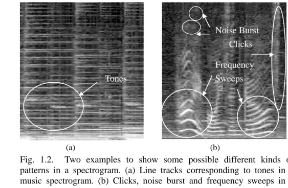
(20) The second proposed method is a non-hierarchical audio classifier, which will first divide an audio stream into clips, each of which contains one-second audio information. Based on the classified clips with smaller length, the proposed method is suitable and can be used to support classification-based audio segmentation. Generally speaking, the spectrogram is a good representation for an audio signal since it is often visually interpretable. By observing a spectrogram, we can find that the energy is not uniformly distributed, but tends to cluster to some patterns. All curve-like patterns are called tracks. Fig. 1.2(a) shows that for a music signal, some line tracks corresponding to tones will exist on its spectrogram. Fig. 1.2(b) shows some patterns including clicks (broadband, short time), noise burst (energy spread over both time and frequency), and frequency sweeps in a song spectrogram. Thus, if. Noise Burst Clicks Frequency Sweeps. Tones. (a). (b). Fig. 1.2. Two examples to show some possible different kinds of patterns in a spectrogram. (a) Line tracks corresponding to tones in a music spectrogram. (b) Clicks, noise burst and frequency sweeps in a song spectrogram. 6.

(21) we can extract some features from a spectrogram to represent these patterns, the classification should be easy. Based on these phenomena, the proposed method will adopt feature selection process to explore the features with the highest discriminative ability to achieve classification purposes and will be used to do audio segmentation. As for the audio segmentation, most of the existing approaches for audio segmentation can be classified into two major paradigms: temporal segmentation and classification-based segmentation. Temporal segmentation (see Fig. 1.3) is a more primitive process than classification-based segmentation since it does not try to interpret the data. By contrast, the classification-based segmentation divides an audio sequence into semantic scenes called “audio scene” and to index them as different audio classes. That is, the approaches via classification usually adopt classification results to achieve segmentation purpose and the performance is dependent on the classification result. In this dissertation, based on the proposed above-mentioned classification method, we will present one classification-based segmentation method to achieve segmentation purpose.. Fig. 1.3.. Temporal segmentation. 7.

(22) 1.2.2 Some Problems of Audio Retrieval In recent years, techniques for audio information retrieval have started emerging as research prototypes. These systems can be classified into two major paradigms [22, 34]. In the first paradigm, the user sings a melody and similar audio files containing that melody are retrieved. This kind of approaches [18] is called “Query by Humming” (QBH). It has the disadvantage of being applicable only when the audio data is stored in symbolic form such as MIDI files. The conversion of generic audio signals to symbolic form, called polyphonic transcription, is still an open research problem in its infancy [16]. Another problem with QBH is that it is not applicable to several musical genres such as Dance music where there is no singable melody that can be used as a query. The second paradigm [9, 15-17, 19-24] is called “Query-by-Example” (QBE), a reference audio file is used as the query and audio files with similar content are returned and ranked by their similarity degree. In order to search and retrieve general audio signals such as the raw audio files (e.g. mp3, wave, etc.) on the web or databases, only the QBE paradigm is currently applicable. There are some disadvantages in the existing QBE audio-retrieval methods.. For. example, the method proposed by Wold, et al. [9] is only suitable for sounds with a single timbre. It is supervised and not adequate to index general audio content. An approach provided in [15] has accuracy varying considerably for different types of. 8.

(23) recording, and the audio segment to be searched should be known a priori in this algorithm. Two MFCC-based (Mel-frequency cepstral coefficients) approaches [16, 21] are not suitable for melody retrieval (e.g. music) since the MFCC-based features do not capture enough information about the pitch content, they characterize the broad shape of the spectrum. Besides, most of the current works only deal with the monophonic sources. Polyphonic music is more common, but it is also more difficult to represent. To solve the above-mentioned shortcomings, in the dissertation, we will present one method for content-based audio retrieval and will also consider polyphonic music. In the dissertation, we will develop our methods based on spectrogram. In the following, we will give a brief review of the generation of the spectrogram.. 1.3 AUDIO REPRESENTATION. We will develop our methods based on spectrogram that is a commonly used representation of an acoustic signal in a three-dimensional (time, frequency, intensity) space known as a time-frequency distribution (TFD) [29]. Traditionally, a spectrogram is displayed with gray levels, where the darkness of a given point is proportional to its energy. The vertical axis in a spectrogram represents frequency and. 9.

(24) the horizontal axis represents time (or frame). To construct a spectrogram, the Short Time Fourier Transform (STFT) is applied. In the following, we will give a brief review of the theories of the Short Time Fourier Transform.. 1.3.1 Short Time Fourier Transform. In general, the input audio signal is first divided into several frames. Each frame contains consecutive n audio signal samples, and two neighboring frames will overlap 50%. Then, the Fourier transform is applied to each frame tapered with a window function in succession (see Fig.1.4). Let s (t ) denote the audio signal and. STFT (τ , ω ) be the result of STFT, that is n −1. τ. t =0. 2. STFT (τ , ω ) = ∑ s (t +. n)r * (t )e − jωt ,. (1.1). where r * (t ) is the window function, τ stands for the frame number, n is the window size and ω is the frequency parameter. Then, the spectrogram, S (τ , ω ) , is. Fourier Transform. Fig. 1.4. Short Time Fourier Transform. 10.

(25) the energy distribution associated with the Short Time Fourier Transform, that is, S (τ , ω ) = 10 log10 (. STFT (τ , ω ) M. )2 ,. (1.2). where M = max STFT (τ , ω ) . τ ,ω. 1.3.2 Multi-resolution Short Time Fourier Transform. Conventionally, in the Short Time Fourier Transform, the TFD is sampled uniformly in time and frequency. However, it is not suitable for the auditory model because the frequency resolution within the human psycho-acoustic system is not constant but varies with frequency [29]. By contrast, in the Multi-resolution Short Time Fourier Transform (MSTFT), the TFD is perceptually tuned, mimicking the time-frequency resolution of the ear. That is, the TFD consists of axes that are non-uniformly sampled. Frequency resolution is coarse and temporal resolution is fine at high frequencies while temporal resolution is coarse and frequency resolution is fine at low frequencies [19]. One example of the tiling in the time-frequency plane is shown in Fig. 1.5 and Fig. 1.6 shows a schematic diagram of the TFD generating using the Multi-resolution Short Time Fourier Transform.. 11.

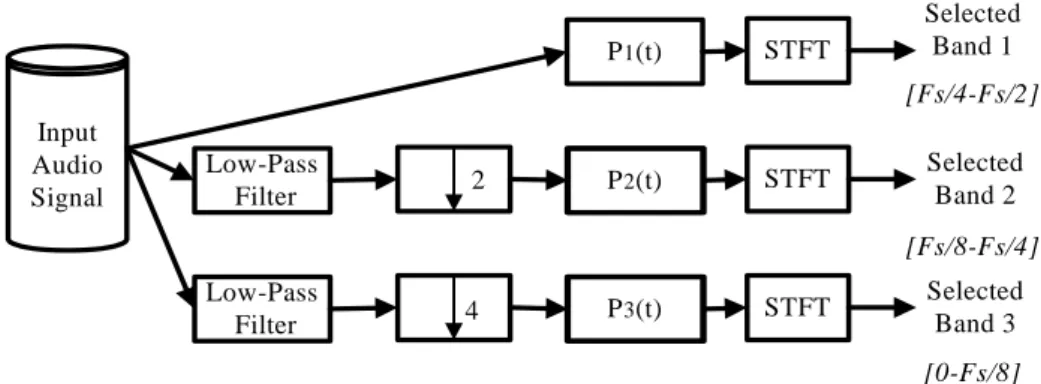
(26) Frequency. Time Fig. 1.5. An example of tiling in the time-frequency plane.. P 1(t). STFT. Selected Band 1 [Fs/4-Fs/2]. Input Audio Signal. Low-Pass Filter. 2. P 2(t). STFT. Selected Band 2 [Fs/8-Fs/4]. Low-Pass Filter. P 3(t). 4. STFT. Selected Band 3 [0-Fs/8]. Fig. 1.6. A schematic diagram of the TFD generating details.. There are three parts in the TFD generating. In the first part, the N -point STFT is applied to the original audio signal P1 (t ) to obtain a spectrogram S1 ( x, y ) . In the second part, a low-pass filter is first applied to P1 (t ) and then the filtered result is downsampled half size to obtain signal P2 (t ) and the N -point STFT is applied to P2 (t ) to obtain a spectrogram S 2 ( x, y ) . In the third part, a low-pass filter is first. applied to P1 (t ) and then the filtered result is downsampled quarter size to obtain signal P3 (t ) and the N -point STFT is applied to P3 (t ) to obtain a spectrogram. 12.

(27) S 3 ( x, y ) . The frequency resolution ∆f j and the analysis time interval T j in S j ( x, y ) can be calculated as follows:. ∆f j =. 1. Fs 1 = , j = 1, 2 ,3. 2 j −1 N T j ⋅. (1.3). Note that the window center at the kth time block in S j ( x, y ) , t kj , is given by. t kj =. k T j , j = 1, 2 ,3. 2. (1.4). Finally, based on S1 ( x, y ) , S 2 ( x, y ) , and S 3 ( x, y ) , a spectrogram I ( x, y ) is obtained according to the following equation: ⎧ S1 ( x, y ), if y ∈ [ FS / 4, FS / 2], x = 0,1,L N f − 1 ; ⎪ ⎪ ⎪S (2i, y ), if y ∈ [ FS / 8, FS / 4], x = 2i,2i + 1., i = 0,1,L N f / 2 − 1 ; I ( x, y ) = ⎨ 2 ⎪ ⎪ S 3 (4i, y ), if y ∈ [ 0 , FS / 8], x = 4i,L,4i + 3, i = 0,1,L N f / 4 − 1 ; ⎪ ⎩ (1.5) where N f is the frame number of P1 (t ) . From Eq. (1.3), we can see that in I(x,y), frequency resolution is coarse and temporal resolution is fine at high frequencies while temporal resolution is coarse and frequency resolution is fine at low frequencies. This means that I(x,y) meets the human psycho-acoustic system.. 1.4 SYNOPSIS OF THE DISSERTATION. The rest of the dissertation is organized as follows. Chapter 2 describes the proposed hierarchical audio classification method. The non-hierarchical audio. 13.

(28) classification and segmentation method based on Gabor wavelets is proposed in Chapter 3. The proposed method of audio retrieval based on Gabor wavelets is described in Chapter 4. Some conclusions and future research directions are drawn in Chapter 5.. 14.

(29) CHAPTER 2 A NEW APPROACH FOR CLASSIFICATION OF GENERIC AUDIO DATA. 2.1. INTRODUCTION. Audio classification [1-14] has many applications in professional media production, audio archive management, commercial music usage, content-based audio/video retrieval, and so on. Several audio classification schemes have been proposed. These methods tend to roughly divide audio signals into two major distinct categories: speech and music. Scherier and Slaney [3] provided such a discriminator. Based on thirteen features including cepstral coefficients, four multidimensional classification frameworks are compared to achieve better performance. The approach presented by Saunders [5] takes a simple feature space and is performed by exploiting the distribution of zero-crossing rate. In general, speech and music have quite different properties in both time and frequency domains. Thus, it is not hard to reach a relatively high level of discrimination accuracy. However, two-type classification for audio data is not enough in many applications, such as content-based video retrieval. 15.

(30) [11]. Recently, video retrieval has become an important research topic. To raise the retrieval speed and precision, a video is usually segmented into several scenes [11,14]. In general, neighboring scenes will have different types of audio data. Thus, if we can develop a method to classify audio data, the classified results can be used to assist scene segmentation. Different kinds of videos will contain different types of audio data. For example, in documentaries, commercials or news report, we can usually find the following audio types: speech, music, speech with musical or environmental noise background, and song. Wyse and Smoliar [7] presented a method to classify audio signals into “music,” “speech,” and “others.” The method was developed for the parsing of news stories. In [8], audio signals are classified into speech, silence, laughter, and non-speech sounds for. the. purpose. of. segmenting. discussion. recordings. in. meetings.. The. above-mentioned approaches are developed for specific scenarios, only some special audio types are considered. The research in [12-14] has taken more general types of audio data into account. In [12], 143 features are first studied for their discrimination capability. Then, the cepstral-based features such as Mel-frequency cepstral coefficients (MFCC), linear prediction coefficients (LPC), etc., are selected to classify audio signals. The authors concluded that in many cases, the selection of features is actually more critical to the classification performance. More than 90% accuracy rate. 16.

(31) is reported. Zhang and Kuo [14] first extracted some audio features including the short-time fundamental frequency and the spectral tracks by detecting the peaks from the spectrum. The spectrum is generated by autoregressive model (AR model) coefficients, which are estimated from the autocorrelation of audio signals. Then, the rule-based procedure, which uses many threshold values, is applied to classify audio signals into speech, music, song, speech with music background, etc. More than 90% accuracy rate is reported. The method is time-consuming due to the computation of autocorrelation function. Besides, many thresholds used in this approach are empirical, they are improper when the source of audio signals is changed. To avoid these disadvantages, in this chapter, we will provide a method with only few thresholds used to classify audio data into five general categories: pure speech, music, song, speech with music background, and speech with environmental noise background. These categories are the basic sets needed in the content analysis of audiovisual data. The proposed method consists of three stages: feature extraction, the coarse-level classification, and the fine-level classification. Based on statistical analysis, four effective audio features are first extracted to ensure the feasibility of real-time processing. They are the energy distribution model, variance and the third moment associated with the horizontal profile of the spectrogram, and the variance of the differences of temporal intervals. Then, the coarse-level audio classification based on. 17.

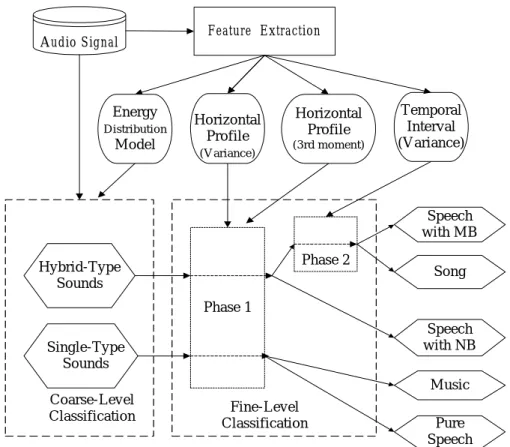
(32) the first feature is conducted to divide audio signals into two categories: single-type and hybrid-type, i.e., with or without background components. Finally, each category is further divided into finer subclass through Bayesian decision function [15]. The single-type sounds are classified into speech and music; the hybrid-type sounds are classified into speech with environmental noise background, speech with music background and song. Experimental results show that the proposed method achieves an accuracy rate of more than 96% in audio classification. The chapter is organized as follows. In Section 2.2, the proposed method will be described. Experimental results and discussion will be presented in Section 2.3. Finally, the summary will be given in Section 2.4.. 2.2. THE PROPOSED METHOD. The system diagram of the proposed audio classification method is shown in Fig. 2.1. It is based on the spectrogram and consists of three phases: feature extraction, the coarse-level classification and the fine-level classification. First, an input audio clip is transformed to a spectrogram as mentioned in Short Time Fourier Transform section (Chapter 1, Section 1.3.1) and four effective audio features are extracted. Figs. 2.2(a) – 2.2(e) show five examples of the spectrograms of music, speech with music. 18.

(33) background, song, pure speech, and speech with environmental noise background, respectively. Then, based on the first feature, the coarse-level audio classification is conducted to classify audio signals into two categories: single-type and hybrid-type. Finally, based on the remaining features, each category is further divided into finer subclasses. The single-type sounds are classified into pure speech and music. The hybrid-type sounds are classified into song, speech with environmental noise background and speech with music background. In the following, the proposed method will be described in details.. A udio Signal. Energy D istribution. M odel. Feature Extraction. H orizontal Profile (V ariance). H orizontal Profile (3rd m om ent). Tem poral Interval (V ariance). Speech w ith M B Phase 2. H ybrid-Type Sounds. Song. Phase 1. Speech w ith N B. Single-Type Sounds. M usic C oarse-Level C lassification. Fine-Level C lassification. Pure Speech. Fig. 2.1. Block diagram of the proposed system, where “MB” and “NB” are the abbreviations for “music background” and “noise background”, respectively.. 19.

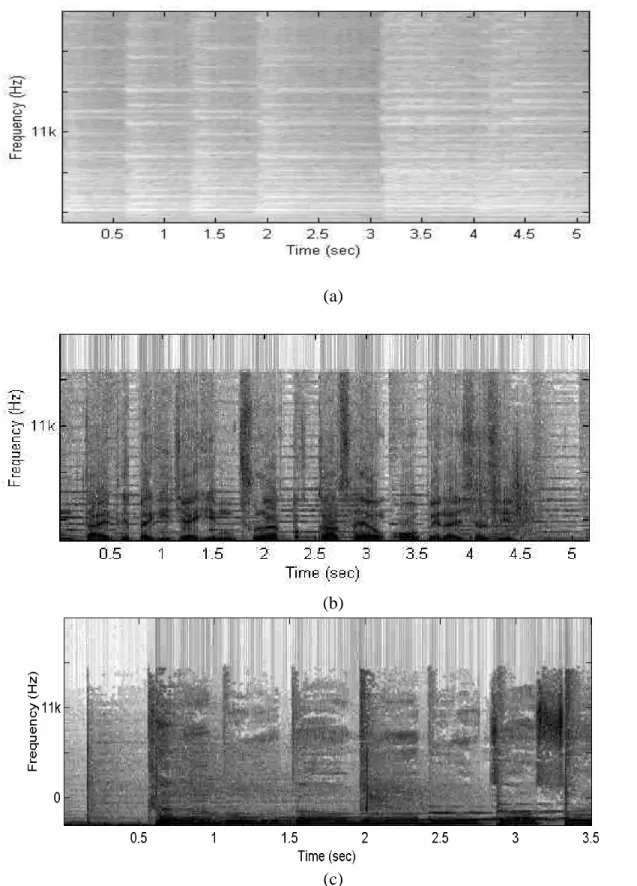
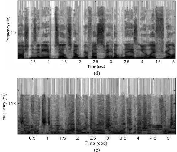
(34) (a). (b). (c) Fig. 2.2. Five spectrogram examples. (a) Music. (b) Speech with music background. (c) Song. (d) Speech. (e) Speech with environmental noise background.. 20.

(35) (d). (e) Fig. 2.2. Five spectrogram examples. (a) Music. (b) Speech with music background. (c) Song. (d) Speech. (e) Speech with environmental noise background. (Continued). 2.2.1. Feature Extraction Phase. Four kinds of audio features are used in the proposed method, they are energy distribution model, variance and the third moment associated with the horizontal profile of the spectrogram, and variance of the differences of temporal intervals (which will be defined later). To get these features, the audio spectrogram for an audio signal is constructed first. Based on the spectrogram, these four features are extracted. 21.

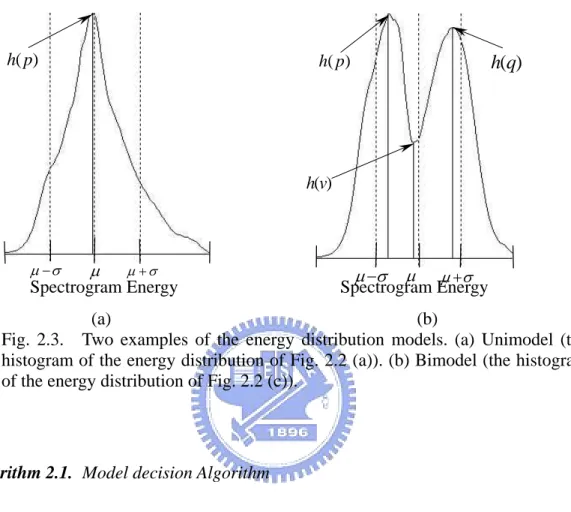
(36) and described as follows.. 2.2.1.1 The Energy Distribution Model. For the purpose of characterizing single-type and hybrid-type sounds, i.e., with or without background components, the energy distribution model is proposed. The histogram of a spectrogram is also called the energy distribution of the corresponding audio signal. In our experiments, we found that there are two kinds of energy distribution models: unimodel and bimodel (see Figs. 2.3 (a) and 2.3 (b)), in audio signals. In Fig. 2.3, the horizontal axis represents the spectrogram energy. For a hybrid-type sound, its energy distribution model is bimodel; otherwise, it is unimodel. Thus, to discriminate single-type sounds from hybrid-type sounds, we only need to detect the type of the corresponding energy distribution model. To reach this, for an audio signal, the histogram of its corresponding spectrogram, h(i ) , is established first. Then, the mean µ and the variance σ 2 of h(i ) are calculated. In general, if µ approaches to the position of the highest peak in h , h(i ) will be a unimodel (see Fig. 2.3 (a)). On the other hand, for a bimodel, dividing h(i ) into two parts from µ , each part will be unimodel (see Fig. 2.3 (b)). Thus, if we find a local peak in each part, these two peaks will not be close. Based on these phenomena, a. 22.

(37) model decision algorithm is provided and described as follows.. h( p). h( p). h(q). h(v). µ −σ µ +σ µ Spectrogram Energy. µ −σ µ µ + σ Spectrogram Energy. (a) (b) Fig. 2.3. Two examples of the energy distribution models. (a) Unimodel (the histogram of the energy distribution of Fig. 2.2 (a)). (b) Bimodel (the histogram of the energy distribution of Fig. 2.2 (c)).. Algorithm 2.1. Model decision Algorithm Input:. The spectrogram S (τ , ω ) of an audio signal.. Output: The model type, T, and two parameters T1, T2.. Step 1.. Establish the histogram, h(i ), i = 0,...,255 , of S (τ , ω ) .. Step 2.. Compute the mean µ and the variance σ 2 of h(i ) .. Step 3.. Find the position p of the highest peak in h(i ) .. Step 4.. If p − µ ≤ 5 , T = unimodel, go to Step 9. Else Use µ to set the search range ℜ p as follows: 23.

(38) ⎧( µ , µ + σ ] , if p < µ ℜp = ⎨ . ⎩ [ µ − σ , µ ) , if p > µ End if.. Step 5.. Find the position q of the highest peak h(q ) within ℜ p .. Step 6.. Find the position v of the lowest valley h(v) in the range between p and q .. Step 7.. Set dst = p − q .. Step 8.. Set T = bimodel if the following two conditions are satisfied Condition 1: dst ≥. σ 2. Condition 2: h(q) ≥. .. 1 6 h( p) and h(q ) ≥ h(v) . 2 5. Else T = unimodel.. Step 9.. Output T and assign µ to T1, µ + σ to T2.. End of Algorithm 2.1.. Through the model decision algorithm described above, the model type for an audio signal can be determined. Note that in the algorithm, except the model type extracted, two parameters, T1 and T2, which will be used later, will be also obtained.. 24.

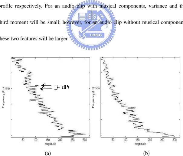
(39) 2.2.1.2 The Horizontal Profile Analysis. In this section, we will base on two facts to discriminate an audio clip with or without music components. One fact is that if an audio clip contains musical components, we can find many horizontal long-line like tracks (see Figs. 2.2 (a) – 2.2 (c)) in its spectrogram. The other fact is that if an audio clip does not contain musical components, most energy in the spectrogram of each frame will concentrate on a certain frequency interval (see Figs. 2.2 (d) – 2.2 (e)). Based on these two facts, two novel features will be derived and used to distinguish music from speech. To obtain these features, the horizontal profile of the audio spectrogram is constructed first. Note that the horizontal profile (see Figs. 2.4 (a) – 2.4 (e)) is defined as the projection of the spectrogram of the audio clip on the vertical axis. Based on the first fact, we can find that for an audio clip with musical components, there will be many peaks in its horizontal profile (see Figs. 2.4 (a) – 2.4 (c)), and the location difference between two adjacent peaks is small and near constant. On the other hand, based on the second fact, we can see that for an audio clip without musical components, only few peaks can be found in its horizontal profile (see Figs. 2.4 (d) – 2.4 (e)), and the location difference between any two successive peaks is larger and variant. Based on the above description, for an audio clip, all peaks, Pi , in its. 25.

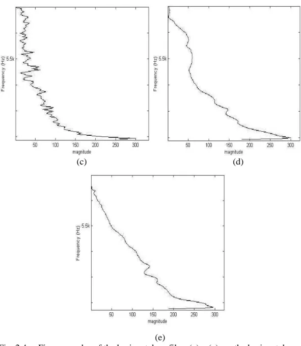
(40) horizontal profile are first extracted; and the location difference, dPi , between any two successive peaks is evaluated. Note that in order to avoid the influence of noise in high frequency, the frequency components above Fs/4 are discarded, where Fs is the sampling rate. Then the variance, v dPi , and the third moment, mdPi , of dPi s are taken as the second and third features and used to discriminate audio clips with or without music components. Note that variance and the third moment stand for the spread and skewness of the location differences of all two successive peaks in the horizontal profile respectively. For an audio clip with musical components, variance and the third moment will be small; however, for an audio clip without musical component, these two features will be larger.. dPi. (a). (b). Fig. 2.4. Five examples of the horizontal profiles. (a) – (e) are the horizontal profiles of Figs. 2(a) - 2(e), respectively.. 26.

(41) (c). (d). (e) Fig. 2.4. Five examples of the horizontal profiles. (a) – (e) are the horizontal profiles of Figs. 2(a) - 2(e), respectively. (Continued). 2.2.1.3 The Temporal Intervals. Up to now, we have provided three features. By processing the audio signals through these features, all audio signals can be classified successfully except the. 27.

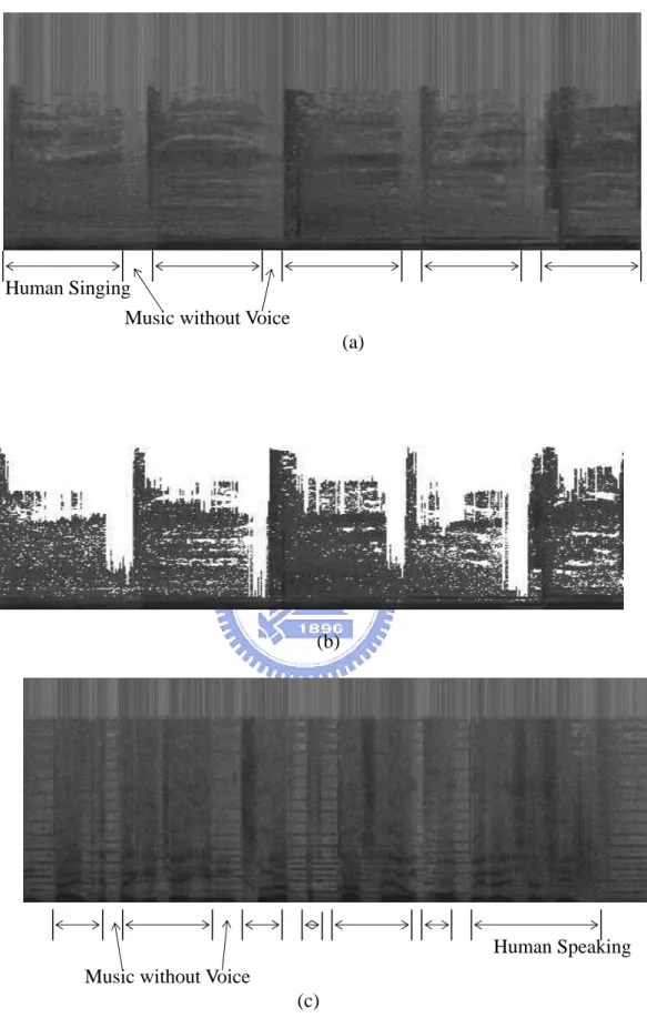
(42) simultaneous speech and music category, which contains two kinds of signals: speech with music background and song. To discriminate these, a new feature is provided. One important characteristic to distinguish them is the duration of the music-voice. The duration of music-voice is defined as the duration of music appearing with human voice simultaneously. That is, two successive durations of music-voice is separated by the duration of a pure music component. For speech with music background, in order to emphasize the message of the talker, the signal energy contribution of voice is greater than the contribution of the music. In general, it is strongly speech-like, the difference between any two adjacent duration of music-voice is variable (see Fig. 2.5 (c)). Conversely, song is usually melodic and rhythmic, the difference between any two adjacent duration of music-voice in song is small and near constant (see Fig. 2.5 (a)). By observing the spectrogram in different frequency bands, we can see that music-voice (i.e. speech and music appears simultaneously) has more energy in the neighboring middle frequency bands, while music without voice will possess more energy in the lower frequency band. These phenomena are shown in Fig. 2.5.. 28.

(43) Human Singing Music without Voice (a). (b). Human Speaking Music without Voice (c) Fig. 2.5. Two examples of the filtered spectrogram. (a) The spectrogram of song. (b) The filtered spectrogram of (a). (c) The spectrogram of speech with music background. (d) The filtered spectrogram of (c).. 29.

(44) (d) Fig. 2.5. Two examples of the filtered spectrogram. (a) The spectrogram of song. (b) The filtered spectrogram of (a). (c) The spectrogram of speech with music background. (d) The filtered spectrogram of (c). (Continued). Based on these phenomena, the property of the duration of each continuous part of the simultaneous speech and music in a sound is used to discriminate the speech with music background from song. First, a novel feature associated with the temporal interval is derived. The temporal interval is defined as the duration of a continuous part of music-voice of a sound. Note that the signal between two adjacent temporal intervals will be music without human voice. Based on the phenomenon of the energy distribution in different frequency bands described previously, an algorithm will be proposed to determine the continuous music-voice parts in a sound. Note that some frequency noises usually exist in an audio clip, i.e., these noises will contribute to those frequencies with lower energy in spectrogram. In order to avoid the influence of frequency noise, a filtering procedure is applied in advance to get rid of those with lower energy. The proposed filtering procedure is provided and described as follows. 30.

(45) Filtering Procedure: 1). Filter out the higher frequency components with lower energy:. For the spectrogram of each frame τ , S (τ , ω ) , find the highest ∧. frequency ω h with S (τ , ω h ) > T 2 . Set S (τ , ω ) = 0 , ∀ ω > ω h . 2). Filter other components: ∧ if S (τ , ω ) < T 1 ⎧ 0, For ω < ω h , S (τ , ω ) = ⎨ otherwise. ⎩S (τ , ω ),. Figs. 2.5 (b) and 2.5 (d) show the filtered spectrograms of Figs. 2.5 (a) and 2.5 (c), respectively. In what follows, we will be interested in how to determine the temporal intervals. Note that an audio clip of the simultaneous speech and music category contains several temporal intervals and some short periods of background music, each of ones will separate two temporal intervals (see Fig. 2.5 (a)). To extract temporal intervals, the entire frequency band [0, Fs/2] is first divided into two subbands of unequal width: [0, Fs/8] and [Fs/8, Fs/2]. Next, for each frame, evaluate the ratio of the non-zero part in each subband to the total non-zero part. If the ratio is larger than 10%, mark the subband. Based on the marked subbands, we can extract the temporal intervals. First, those neighboring frames with the same marked subbands are merged to form a group. 31.

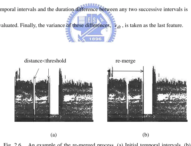
(46) If the higher subband (i.e., [Fs/8, Fs/2]) in a group is marked, the group will be regarded as a part of music-voice (also called raw temporal interval). That is, a temporal interval is a sequence of frames with higher energy in higher subband. Since the results obtained after filtering procedure are usually sensitive to unvoiced speech and slight breathing, a re-merged process is then applied to the raw temporal intervals. During the re-merged process, two neighboring intervals are merged if the distance between them is less than a threshold. Fig. 2.6 shows an example of the re-merge process. Once we complete this step, we will obtain a set of temporal intervals and the duration difference between any two successive intervals is evaluated. Finally, the variance of these differences, vdt , is taken as the last feature.. distance<threshold. re-merge. (a). (b). Fig. 2.6. An example of the re-merged process. (a) Initial temporal intervals. (b) Result after re-merged process.. 32.

(47) 2.2.2. Audio Classification. Since there are some similar properties among most of the five classes considered, it is hard to find distinguishable features for all of these five classes. To treat this problem, a hierarchical system is proposed. It will do coarse-level classification first, then the fine-level classification is performed. To meet the aim of on-line classification, features described above are computed on the fly with incoming audio data.. 2.2.2.1 The Coarse-Level Classification. The aim of coarse-level audio classification is to separate the five classes into two categories such that we can find some distinguishable features in each category. Based on the energy distribution model, audio signals can be first classified into two categories: single-type and hybrid-type, i.e., with or without background components. Single-type sounds contain pure speech and music. And hybrid-type sounds contain song, speech with environmental noise background and speech with music background.. 33.

(48) 2.2.2.2 The Fine-Level Classification. The coarse-level classification stage yields a rough classification for audio data. To get the finer classification result, the fine-level classifier is conducted. Based on the extracted feature vector X, the classifier is designed using a Bayesian approach under the assumption that the distribution of the feature vectors in each class wk is a multidimensional Gaussian distribution N k (mk , C k ) . The Bayesian decision function [15] for class wk , d k ( X ) has the form: 1 1 d k ( X ) = ln P( wk ) − ln C k − ( X − mk ) T C k−1 ( X − mk ) , 2 2. (2.3). where mk and C k are the mean vector and covariance matrix of X, and P( wk ) is the priori probability of class wk . For a piece of sound, if its feature vector X satisfies. d i ( X ) > d j ( X ) for all j ≠ i , it is assigned to class wi . The fine-level classifier consists of two phases. During the first phase, we take ( v dPi , mdPi ) as the feature vector X and apply Bayesian decision function to each of the two coarse-level classes separately. For each audio signal of the single-type class, we can successfully classify it as music or pure speech. And the classification is well done without needing any further processing. For that of the hybrid-type sounds, which may be speech with environmental noise background, speech with music. 34.

(49) background or song, the same procedure is applied. Speech with environmental noise background is distinguished and what left in the first phase is the subclass including speech with music background and song. An additional process is needed to do further classification for the subclass. To do this, the Bayesian decision function with the feature vdt is applied. And we can successfully classify each signal in this subclass as speech with music background or song.. 2.3. EXPERIMENTAL RESULTS. In order to do comparison, we have collected a set of 700 generic audio pieces of different types of sound according to the collection rule described in [14] as the testing database. Care was taken to obtain a wide variation in each category, and most of clips are taken from MPEG-7 content set [14, 17]. For single-type sounds, there are 100 pieces of classical music played with varied instruments, 100 other music pieces of different styles (jazz, blues, light music, etc.), and 200 clips of pure speech in different languages (English, Chinese, Japanese, etc.). For hybrid-type sounds, there are 200 pieces of song sung by male, female, or children, 50 clips of speech with background music (e.g., commercials, documentaries, etc.), and 50 clips of speech with environmental noise (e.g., sport broadcast, news interview, etc.). These audio. 35.

(50) clips (with duration from several seconds to no more than half minute) are stored as 16-bit per sample with 44.1 kHz sampling rate in the WAV file format.. 2.3.1 Classification Results. Tables I and II show the results of the coarse-level classification and the final classification results, respectively. From Table II, it can be seen that the proposed classification approach for generic audio data can achieve an accuracy rate of more than 96% by using the testing database. The training is done using 50% of randomly selected samples in each audio type, and the test is operated on the remaining 50%. By changing training set several times and evaluating the classification rates, we find that the performance of the system is stable and independent on the particular test and training sets. Note that the experiments are carried out on a Pentium II 400 PC/Windows 2000, it needs less than one twentieth of the time required to play the audio clip for processing an audio clip. The only computational expensive part is the spectrogram, and the other processing is simple by comparison (e.g. variances, peak finding, etc). In order to do comparison, we also like to cite the efficiency of the existing system described in [14], which also includes the five audio classes considered in our method and uses similar database to ours. The authors of [14] report. 36.

(51) that less than one eighth of the time required to play the audio clip are needed to process an audio clip. They also report that their accuracy rates are more than 90%.. TABLE 2.1 COARSE-LEVEL CLASSIFICATION RESULTS. Audio Type. Number. Correct Rates. Single-Type. Pure Speech. 200. 100%. Sounds. Pure Music. 200. 100%. Hybrid-type. Song. 200. 100%. Sounds. Speech with MB. 50. 100%. Speech with NB. 50. 100%. TABLE 2.2 FINAL CLASSIFICATION RESULTS. Audio Type. Number. Correct Rates. Single-Type. Pure Speech. 200. 100%. Sounds. Pure Music. 200. 97.6%. Hybrid-type. Song. 200. 98.53%. Sounds. Speech with MB. 50. 96.5%. Speech with NB. 50. 100%. 37.

(52) 2.4. SUMMARY. In this chapter, we have presented a new method for the automatic classification of generic audio data. An accurate classification rate higher than 96% was achieved. Two important and distinguishing features compared with previous work in the proposed scheme are the complexity and running time. Although the proposed scheme covers a wide range of audio types, the complexity is low due to the easy computing of audio features, and this makes online processing possible. Besides the general audio types such as music and speech tested in existing work, we have taken hybrid-type sounds (speech with music background, speech with environmental noise background, and song) into account. While current existing approaches for audio content analysis are normally developed for specific scenarios, the proposed method is generic and model free. Thus, our method can be widely applied to many applications.. 38.

(53) CHAPTER 3 A NEW APPROACH FOR AUDIO CLASSIFICATION AND SEGMENTATION USING GABOR WAVELETS AND FISHER LINEAR DISCRIMINATOR. 3.1. INTRODUCTION. In recent years, audio, as an important and integral part of many multimedia applications, has been gained more and more attentions. Rapid increase in the amount of audio data demands for an efficient method to automatically segment or classify audio stream based on its content. Many studies on audio content analysis [1-14] haven been proposed. A speech/music discriminator was provided in [3], based on thirteen features including cepstral coefficients, four multidimensional classification frameworks are compared to achieve better performance. The approach presented by Saunders [5] takes a simple feature space, it is performed by exploiting lopsidedness of the distribution of zero-crossing rate, where speech signals show a marked rise that is not common for music signals. In general, for speech and music, it is not hard to reach a relatively high level of discrimination accuracy since they have quite different. 39.

(54) properties in both time and frequency domains. Besides speech and music, it is necessary to take other kinds of sounds into consideration in many applications. The classifier proposed by Wyse and Smoliar [7] classifies audio signals into “music,” “speech,” and “others.” It was developed for the parsing of news stories. In [8], audio signals are classified into speech, silence, laughter, and non-speech sounds for the purpose of segmenting discussion recordings in meetings. However, the accuracy of the segmentation resulted using this method varies considerably for different types of recording. Besides the commonly studied audio types such as speech and music, the research in [12-14] has taken into account hybrid-type sounds, e.g., the speech signal with the music background and the singing of a person, which contain more than one basic audio type and usually appear in documentaries or commercials. In [12], 143 features are first studied for their discrimination capability. Then, the cepstral-based features such as Mel-frequency cepstral coefficients (MFCC), linear prediction coefficients (LPC), etc., are selected to classify audio signals. Zhang and Kuo [14] extracted some audio features including the short-time fundamental frequency and the spectral tracks by detecting the peaks from the spectrum. The spectrum is generated by autoregressive model (AR model) coefficients, which are estimated from the autocorrelation of audio signals. Then, the rule-based procedure, which uses many threshold values, is applied to classify audio. 40.

(55) signals into speech, music, song, speech with music background, etc. Accuracy of above 90% is reported. However, this method is complex and time-consuming due to the computation of autocorrelation function. Besides, the thresholds used in this approach are empirical, they are improper when the source of audio signals is changed. In this chapter, we will provide two classifiers, one is for speech and music (called two-way); the other is for five classes (called five-way) that are pure speech, music, song, speech with music background, and speech with environmental noise background. Based on the classification results, we will propose a merging algorithm to divide an audio stream into some segments of different classes. One basic issue for content-based classification of audio sound is feature selection. The selected features should be able to represent the most significant properties of audio sounds, and they are also robust under various circumstances and general enough to describe various sound classes. The issue in the proposed method is addressed in the following: first, some perceptual features based on the Gabor wavelet filters [15-16] are extracted as initial features, then Fisher Linear Discriminator (FLD) [17] is applied to these initial features to explore the features with the highest discriminative ability. Note that FLD is a tool for multigroup data classification and dimensionality. 41.

(56) reduction. It maximizes the ratio of between-class variance to within-class variance in any particular data set to guarantee maximal separability. Experimental results show that the proposed method can achieve an accuracy rate of discrimination over 98% for a two-way speech/music discriminator, and more than 95% for a five-way classifier which uses the same database as that used in the two-way discrimination. Based on the classification result, we can also identify scene breaks in audio sequence quite accurately. Experimental results show that our method can detect more than 95% of audio type changes. These results demonstrate the capability of the proposed audio features for characterizing the perceptual content of an audio sequence. The rest of the chapter is organized as follows. In Section 3.2, the proposed method is described in details. Experimental results and discussion are presented in Section 3.3. Finally, in Section 3.4, we give a summary.. 3.2. THE PROPOSED METHOD. The block diagram of the proposed method is shown in Fig. 3.1. It is based on the spectrogram and consists of five phases: time-frequency distribution (TFD) generation, initial feature extraction, feature selection, classification and segmentation. First, the input audio is transformed to a spectrogram, I ( x, y ) , as mentioned in. 42.

(57) Multi-resolution Short Time Fourier Transform section (Chapter 1, Section 1.3.2). Second, for each clip with one-second window, some Gabor wavelet filters will be applied to the resulting spectrogram to extract a set of initial features. Third, based on the extracted initial features, the Fisher Linear Discriminator (FLD) is used to select the features with the best discriminative ability and also to reduce feature dimension. Fourth, based on the selected features, classification method is then provided to classify each clip. Finally, based on the classified clips, a segmentation technique is presented to identify scene breaks in each audio stream. In what follows, we will describe the details of the proposed method.. Music Two-way feature selection and classification. Audio Signal. Speech. Pure Music. TFD generation. Initial feature extraction. Five-way feature selection and classification. Two-way segmentation. Segments. Song. Pure Speech. Five-way segmentation. Speech with MB Speech with NB. Segments. Fig. 3.1. Block diagram of the proposed method, where “MB” and “NB” are the abbreviations for “music background” and “noise background”, respectively.. 43.

(58) 3.2.1 Initial Feature Extraction. Generally speaking, the spectrogram is a good representation for the audio since it is often visually interpretable. By observing a spectrogram, we can find that the energy is not uniformly distributed, but tends to cluster to some patterns (see Fig. 3.2 (a), 3.2 (b)). All curve-like patterns are called tracks [31]. Fig. 3.2 (a) shows that for a music signal, some line tracks corresponding to tones will exist on its spectrogram. Fig. 3.2 (b) shows some patterns including clicks (broadband, short time), noise burst (energy spread over both time and frequency), and frequency sweeps in a song spectrogram.. Tones. Noise Burst Clicks Frequency Sweeps. (a) (b) Fig. 3.2. Two examples to show some possible different kinds of patterns in a spectrogram. (a) Line tracks corresponding to tones in a music spectrogram. (b) Clicks, noise burst and frequency sweeps in a song spectrogram.. 44.

(59) Thus, if we can extract some features from a spectrogram to represent these patterns, the classification should be easy. Smith and Serra [32] proposed a method to extract tracks from a STFT spectrogram. Once the tracks are extracted, each track is classified. However, tracks are not well suited for describing some kinds of patterns such as clicks, noise burst and so on. To treat all kinds of patterns, a richer representation is required. In fact, these patterns contain various orientations and spatial scales. For example, each pattern formed by lines (see Fig. 3.2 (a)) will have a particular line direction (corresponding to orientation) and width (corresponding to spatial scale) between two adjacent lines; each pattern formed by curves (see Fig. 3.2 (b)) contains multiple line directions and a particular width between two neighboring curves. Since Gabor wavelet transform provides an optimal way to extract those orientations and scales [27], in this chapter, we will use the Gabor wavelet functions to extract some initial features to represent those patterns. The detail will be described in the following section.. 3.2.1.1 Gabor Wavelet Functions and Filters Design. Two-dimensional Gabor kernels are sinusoidally modulated Gaussian Functions. Let g ( x, y ) be the Gabor kernel, its Fourier Transform G (u, v) can be defined as. 45.

(60) follows [28]: −1 x2 y2 ) exp[ ( g ( x, y ) = ( + ) + 2π j ω x] , 2πσ xσ y 2 σ x2 σ 2y. (3.1). − 1 (u − ω ) 2 v 2 [ + ]) , 2 σ u2 σ v2. (3.2). 1. G (u , v) = exp(. where σ u =. 1 2πσ x. and σ v =. 1 2πσ y. and ω is the center frequency.. Gabor wavelets are sets of Gabor kernels which will be applied to different subbands with different orientations. It can be obtained by appropriate dilations and rotations of g ( x, y ) through the following generating functions [28]:. g mn ( x, y ) = a − m g ( x' , y ' ) , a>1, m, n = integer, x' = a − m ( x cosθ + y sin θ ) , and y ' = a − m (− x sin θ + y cosθ ) ,. ω a=( h. ωl. 1 S ) −1 ,. (3.4). σ u = ((a − 1) ω h ) /((a + 1) 2 ln 2 ) ,. (3.5) −1. (2 ln 2) 2 −σ u2 2 σ2 ] σ v = tan( π )[ω h − 2 ln 2( u )][2 ln 2 − 2k ωh ω2 h. where θ =. (3.3). (3.6) ,. nπ , n = 0,1,L , K − 1. , m = 0,1, L, S − 1. , K is the total number of K. orientations, S is the number of scales in the multi-resolution decomposition, ω h and ω l are the highest and the lowest center frequency, respectively. In this chapter, we set ω l = 3 , ω h = 3 , K = 6 and S = 7 . 64 4. 46.

(61) 3.2.1.2 Feature Estimation and Representation. To extract the audio features, each Gabor wavelet filter, g mn ( x, y ) , is first applied to the spectrogram I ( x, y ) to get a filtered spectrogram, Wmn ( x, y ) , as Wmn ( x, y ) = ∫ I ( x − x1 , y − y1 ) g. mn. * ( x1 , y1 )dx1dy1 ,. (3.7). where * indicates the complex conjugate. The above filtering process is executed by FFT (fast Fourier Transform). That is Wmn ( x, y ) = F −1{F {g mn ( x, y )}⋅ F {I ( x, y )}}.. (3.8). Since peripheral frequency analysis in the ear system roughly follows a logarithmic axis, in order to keep with this way, the entire frequency band [0, Fs/2] is divided into six subbands of unequal width: F1=[0, Fs/64], F2=[Fs/64, Fs/32], F3=[Fs/32, Fs/16], F4=[Fs/16, Fs/8], F5=[Fs/8, Fs/4], and F6=[Fs/4, Fs/2]. In our experiments, high frequency components above Fs/4 (i.e., subband [Fs/4, Fs/2]) are discarded to avoid the influence of noise. Then, for each interested subband Fi , the directional histogram, H i (m, n) , is defined to be H i (m, n) =. N i (m, n) 5. ∑ N i (m, n). , i = 0,L,4 ,. (3.9). n=0. ⎧1, if Wmn ( x, y ) > Tm and y ∈ Fi i Wmn , ( x, y ) = ⎨ otherwise ⎩0, i N i (m, n) = ∑∑ Wmn ( x, y ), x. y. 47. (3.10). (3.11).

(62) where m = 0,L,6. and n = 0,L,5. . Note that N i (m, n) is the number of pixels in the filtered spectrogram Wmn ( x, y ) at subband Fi , scale m and direction n with value larger than threshold Tm . Tm is set as Tm = µ m + σ m .. (3.12). where 1 ⎛ 5 ⎞2 5 µ m = ∑ ∑ ∑ Wmn ( x, y ) N m , σ m = ⎜ ∑ ∑ ∑ (Wmn ( x, y ) − µ m ) 2 / N m ⎟ , ⎜ ⎟ n=0x y ⎝n = 0 x y ⎠. and N m is the number of pixels over all the 6 filtered spectrogram Wmn ( x, y ) with scale m. An initial feature vector, f , is now constructed using H i (m, n) as feature components. Recall that in our experiments, we use seven scales (S=7), six orientations (K=6) and five subbands, this will result in a 7 × 6 × 5 dimensional initial feature vector f = [ H 0 (0,0), H 0 (0,1),L, H 4 (6,5)]T .. (3.13). 3.2.1.3 Feature Selection and Audio Classification. The initial features are not used directly for classification since some features give poor separability among different classes and inclusion of these features will. 48.

(63) lower down classification performance. In addition, some features are highly correlated so that redundancy will be introduced. To remove these disadvantages, in this chapter, the Fisher Linear Discriminator (FLD) is applied to the initial features to find those uncorrected features with the highest separability. Before describing FLD, two matrices, between-class scatter and within-class scatter, will first be introduced. The within-class scatter matrix measures the amount of scatter between items in the same class and the between-class scatter matrix measures the amount of scatter between classes. i is defined as For the i th class, the within-class scatter matrix S w. ∑ ( xki − µ i )( xki − µ i )T ,. i Sw =. (3.14). x ki ∈ X i. the total within-class scatter matrix S w is defined as C. i Sw = ∑ Sw ,. (3.15). i =1. and the between-class scatter matrix S b is defined as C. S b = ∑ N i ( µ i − µ )( µ i − µ )T ,. (3.16). i =1. where µ i is the mean of class X i , N i is the number of samples in class X i , x ki is the kth sample in X i , and C is the number of classes. In FLD, a matrix Vopt = {v1 , v 2 , L , vC −1} is first chosen, it satisfies the following equation: 49.